Abstract

Cosmological solutions for a pressureless fluid in the Brans-Dicke theory exhibit asymptotical accelerated phase for some range of values of the parameter $\omega$, interpolating a matter dominated phase and an inflationary phase. The effective gravitational coupling is negative. We test this model against the supernovae type Ia data. The fitting of the observational data is slightly better than that obtained from the $\Lambda CDM$ model. We make some speculations on how to reconcile the negative gravitational coupling in large scale with the local tests. Some considerations on the structure formation problem in this context are also made.

PACS number(s): 04.20.Cv., 04.20.Me

1 Introduction

The accumulation of supernovae type Ia data seems to confirm that the universe is today in an accelerated phase [1, 2]. The first indications of this accelerated phase came from the analysis of about $50$ supernovae. Today, the data are approaching 300 supernovae [3, 4], and those first conclusions, for the moment, are confirmed. The theoretical explanation of this surprising result is one of the most important challenge in cosmology. In order to obtain an accelerated phase, a repulsive gravitational effect must be obtained. Generally, this is achieved by introducing an exotic fluid which exhibits a negative pressure today, called dark energy (for a recent review, see reference [5]). The most natural candidate is a cosmological constant, since it is an inevitable consequence of considering quantum fields in a curved space-time. But, the cosmological constant proposal faces a major difficulty: the theoretical predicted value surpass the value induced by observation by 120 order of magnitudes. This discrepancy can be alleviated, but not solved, by considering, for example, supersymmetric theories. Moreover, the introducing of a cosmological constant today does not explain the coincidence problem, the fact that the universe begun to accelerated very recently, after the completion of formation of local structures like galaxies and clusters of galaxies.

Many other alternatives to the cosmological constant have been presented in the literature. In the quintessence program, a self-interacting scalar field is considered [6, 7]. The potential for the scalar field is such that initially the pressure is positive, in order to allow the formation of local structures, becoming latter negative, driving the acceleration of the universe. The coincidence problem may be addressed in this case. However, fine tuning is required. However, some more natural potentials have been determined using supergravity theories [8]. Other dark energy models appear in the literature: k-essence [9], Chaplygin gas [10, 11], viscous fluid [12], etc. Here, we explore another possibility: the acceleration phase could be generated by a non-minimal coupling between a scalar field and the gravitational term.

The paradigm of a scalar-tensor theory with non-minimal coupling is the Brans-Dicke theory, which is characterized by the Lagrangian

$$L=\sqrt{-g}\biggr{[}\phi R-\omega\frac{\phi_{;\rho}\phi^{;\rho}}{\phi}\biggl{]}+L_{m}\quad,$$ (1)

where $\omega$ is a coupling parameter and $L_{m}$ is a matter Lagrangian. Local tests at level of the solar system and stellar binary systems, restrict $\omega$ to be larger than around $1,000$ [13]. This makes the predictions of the Brans-Dicke theory almost indistinguishable of those coming from general relativity. The scalar field $\phi$ is related to the inverse of the gravitational coupling $G$. Some recent interesting proposals address the possibility that the gravitational coupling can depend on the scale, having different value at local and at cosmological scales [14, 15]. If such scale-dependent gravitational coupling can be satisfactorily implemented, it is possible to have smaller values for the parameter $\omega$ at cosmological scales, obtaining scenarios that differ substantially from those obtained from general relativity, while agreement with local tests is preserved. Studies of quantum effects in gravitational theories, and their consequence for the behaviour of the gravitational coupling, have strengthened those proposals [16, 17].

In reference [18], general cosmological solutions for a flat universe in the Brans-Dicke theory were determined. For a pressureless fluid, such solutions can interpolate a decelerating phase with an accelerated phase. This is an example of how cosmological models in Brans-Dicke theory may differ substantially from the standard cosmological model: using general relativity such interpolation can just be obtained through introduction of an exotic fluid. However, the price to pay is not negligible: the Brans-Dicke parameter must takes values in the interval $-3/2<\omega<-4/3$, implying that the effective gravitational coupling is negative. The possibility of a scale-dependent gravitational coupling may render, however, such scenarios attractive.

These solutions with a late accelerated phase were studied in reference [19]. Here we make a step further: a comparison with the supernovae type Ia data is made, using the ”gold sample”. This Brans-Dicke late accelerated model gives better agreement with the observational data than the $\Lambda CDM$ model. The best fitting for the Brans-Dicke parameter and the Hubble parameter $h$ are obtained, indicating $\omega\approx-1.5$ and $h\approx 0.6$. The approach here differs from others existing in the literature which studies accelerated models in Brans-Dicke theory [20, 21, 22, 23, 24, 25, 26, 27] by the fact that no other ingredient is introduced, like a potential term for the scalar field. But, the model requires an effective mechanism that leads to a repulsive gravitational coupling at cosmological scales, while keeping it attractive at local scales.

This article is organized as follows. In next section, the pressureless Brans-Dicke cosmological model is revised. In section $3$, the comparison with the supernovae type Ia ”gold sample” is made. In section $4$ we present our conclusions.

2 Late accelerated phase in the Brans-Dicke cosmological model

Let us consider a flat Brans-Dicke cosmology, with the universe filled with pressureless matter. The equations of motion resulting from the Lagrangian (1) are:

$$3\biggr{(}\frac{\dot{a}}{a}\biggl{)}^{2} = \frac{8\pi\rho}{\phi}+\frac{\omega}{2}\biggr{(}\frac{\dot{\phi}}{\phi}\biggl{)}-3\frac{\dot{a}}{a}\frac{\dot{\phi}}{\phi}\quad,$$ (2)

$$\ddot{\phi}+3\frac{\dot{a}}{a}\dot{\phi} = \frac{8\pi\rho}{3+2\omega}\quad,$$ (3)

$$\dot{\rho}+3\frac{\dot{a}}{a}\rho = 0\quad.$$ (4)

The last equation leads to $\rho=\rho_{0}a^{-3}$. Inserting this relation in (3), we find the first integral, $\dot{\phi}=\frac{8\pi\rho t}{3+2\omega}C$, where $C$ is a constant.

Following [28], we can define an auxiliary function $u$, satisfying the relation

$$\frac{\dot{u}}{u}=-3\frac{\dot{a}}{a}+\frac{2}{t}-\frac{u}{t}$$ (5)

which, in view of the equations of motion, results in the integral relation

$$\int\frac{du}{u[u+4\pm s\sqrt{u^{2}+4u}]}=2\ln(t-t_{c})\quad,$$ (6)

where $s=3\sqrt{1+\frac{2}{3}\omega}$. This integral relation has three critical points $u=0$, $u=-4$ and $u=\frac{2}{4+3\omega}$. The first one gives non physical results, while the second one leads to $a\propto t^{2}$ for any value of $\omega$. For this last case, $\frac{8\pi\rho}{\phi}=-4(3+2\omega)$. However, the fact that the evolution of the scale factor does not depend on $\omega$ makes this solution not very interesting.

The third critical point of (6) leads to a particular solution in terms of power law function (choosing $t_{c}=0$):

$$a=a_{0}t^{\frac{2+2\omega}{4+3\omega}}\quad,\quad\phi=\phi_{0}t^{\frac{2}{4+3\omega}}\quad.$$ (7)

A more general solution may be obtained through integration of (6). This has been done in [18], resulting in the general flat solutions

$$a = a_{0}(t-t_{-})^{\frac{1+\omega\pm\sqrt{1+\frac{2}{3}\omega}}{4+3\omega}}(t-t_{+})^{\frac{1+\omega\mp\sqrt{1+\frac{2}{3}\omega}}{4+3\omega}}\quad,$$ (8)

$$\phi = \phi_{0}(t-t_{-})^{\frac{1\mp 3\sqrt{1+\frac{2}{3}\omega}}{4+3\omega}}(t-t_{+})^{\frac{1\pm 3\sqrt{1+\frac{2}{3}\omega}}{4+3\omega}}\quad,$$ (9)

where $t_{\pm}=t_{c}+A(s\pm 1)$, $A$ being another integration constant. Since $t_{+}>t_{-}$ , $t=t_{+}$ may be identified with the initial time.

The solutions presented above have the following properties. For $t\rightarrow t_{+}$, they reduce to

$$a = a_{0}t^{\frac{1+\omega\mp\sqrt{1+\frac{2}{3}\omega}}{4+3\omega}}\quad,$$ (10)

$$\phi = \phi_{0}t^{\frac{1\pm 3\sqrt{1+\frac{2}{3}\omega}}{4+3\omega}}\quad,$$ (11)

while for $t>>t_{+}$, they take the form

$$a=a_{0}t^{\frac{2+2\omega}{4+3\omega}}\quad,\quad\phi=\phi_{0}t^{\frac{2}{4+3\omega}}\quad.$$ (12)

Concerning the possible scenarios, the solutions have the following properties:

1. For $\omega>-\frac{4}{3}$: The universe has a decelerated expansion during all its evolution.

2. For $\omega<-\frac{3}{2}<\omega<-\frac{4}{3}$ there are two regimes:

   1. For the positive upper sign, initially the universe has a subluminal expansion, followed by a superluminal expansion;

   2. For the negative lower sign, the universe has an accelerated phase during all its evolution.

Is the case (2.a) that it will interest us. In such a case, the interpolation between a decelerated phase and an accelerated phase can be achieved. However, there is high price to pay in order to obtain such a simple qualitative realization of the accelerated expansion today without introducing any kind of exotic matter: the gravitational coupling is negative. In fact, the gravitational coupling is related to the scalar field $\phi$ by the relation [28]

$$G=\frac{4+2\omega}{4+3\omega}\frac{1}{\phi}\quad.$$ (13)

Hence, for $-3/2<\omega<-4/3$, $G<0$.

The most popular model to explain the current acceleration of the universe is the $\Lambda CDM$ model. The matter content is a pressureless fluid and the cosmological constant. For a spatial flat case, the Einstein’s equation reduce to

$$3\biggr{(}\frac{\dot{a}}{a}\biggl{)}^{2}=8\pi G\rho_{m}+\Lambda\quad,$$ (14)

where $\rho_{m}=\rho_{m0}a^{-3}$. This equation admits the solution

$$a=\biggr{(}\frac{3M}{4\Lambda}\biggl{)}^{\frac{1}{3}}\sinh^{\frac{2}{3}}\sqrt{\frac{3\Lambda}{4M}}t\quad.$$ (15)

where $M=8\pi G\rho_{m0}/3$. The asymptotical behaviour are

$$t\rightarrow 0\quad \Rightarrow \quad a\propto t^{\frac{2}{3}}\quad,$$ (16)

$$t\rightarrow\infty\quad \Rightarrow \quad a\propto e^{\sqrt{\frac{3\Lambda}{4M}}t}\quad.$$ (17)

As expected, initially the scale factor describes a dust dominated universe, and later a cosmological constant dominated universe.

3 Comparing with the supernovae type Ia data

We intend now to compare the background model for the flat pressureless fluid Brans-Dicke cosmology with the supernovae type Ia data. This is made through the computation of the luminosity distance function, given by

$$D_{L}=\frac{a_{0}}{a}r,$$ (18)

where $a_{0}$ is the value of the scale factor today, $a$ is the value of the scale factor at the time of the emission of the radiation, and $r$ is the co-moving radial distance. From now on, we fix $a_{0}=1$. With this normalization choice, the scale factor at a given moment $t$ is related with the redshift $z$ by

$$a=\frac{1}{1+z}\quad.$$ (19)

Hence, the luminosity distance can be expressed as [28]

$$D_{L}=(1+z)r\quad.$$ (20)

Usually, the observational data are expressed in terms of the distance moduli given by

$$\mu_{0}=5\log\biggr{(}\frac{D_{L}}{Mpc}\biggl{)}+25\quad.$$ (21)

In general the task now would consist in using the Friedmann equation as

$$\biggr{(}\frac{\dot{a}}{a}\biggl{)}^{2}=\frac{8\pi G}{3}\sum_{i=1}^{n}\rho_{i}\quad,$$ (22)

where $\rho_{i}$ are the different matter components. If each of this component obeys a separate conservation equation, it can express as $\rho_{i}=\rho_{i0}a^{-3(1+\alpha_{i})}$, where $\alpha_{i}$ is the barotropic equation of state (supposed to be constant) defined by $p_{i}=\alpha_{i}\rho_{i}$. Using then the relation between the scale factor and $z$, the luminosity function can be expressed as an integral over $z$ which depends on the density parameter today for each fluid. This procedure is detailed, for example, in reference [29]. It must be remarked also that the expression (21) must be modified for the case the gravitational coupling varies with $z$, as reported in references [30, 31, 32]. However, in the case we consider here, the local physics is supposed to be given by general relativity, the Brans-Dicke modifications intervening at cosmological scales only. Hence, with this assumption, the expression (21) may be still used safely.

For the Brans-Dicke cosmological model presented in the previous section the procedure outlined above becomes impossible to be applied due to the non-minimal coupling between gravity and the scalar field. But, we can use the relation

$$r=c\int_{t_{e}}^{t_{0}}\frac{dt}{a(t)}\quad,$$ (23)

where $t_{e}$ is the emission time for the source at the redshift $z$ and $t_{0}$ is the present time, together with the normalization condition $a(t_{0})=a_{0}=1$. The expression (8) may be rewritten as

$$a(x)=\biggr{(}\frac{x-\frac{t_{+}}{t_{0}}}{1-\frac{t_{+}}{t_{0}}}\biggl{)}^{r+s}x^{r-s}\quad,$$ (24)

$$r=\frac{1+\omega}{4+3\omega}\quad,\quad s=\frac{\sqrt{1+\frac{2}{3}\omega}}{4+3\omega}\quad,\quad x=\frac{t}{t_{+}}\quad.$$ (25)

The present time may be determined through the definition for the Hubble parameter

$$H=\frac{\dot{a}}{a}=\frac{2rt-(r-s)t_{+}}{(t-t_{+})t}\quad.$$ (26)

Evaluated for today, $t=t_{0}$, when $H=H_{0}$, this leads to the expression

$$t_{0}=\frac{(H_{0}t_{+}+2r)\pm\sqrt{(H_{0}t_{+}+2r)^{2}-4H_{0}(r-s)t_{+}}}{2H_{0}}\quad,$$ (27)

where $H_{0}=100\,h\,km/(Mpc.s)$, $h$ being one of the parameters to be determined. Hence, the luminosity distance is given by,

$$D_{L}=(1+z)ct_{0}\int_{x}^{1}\frac{dy}{a(y)}\quad,$$ (28)

where $y$ is the integration variable. The same procedure is used for the $\Lambda CDM$ model described in the end of the previous section.

In order to compare with the supernovae data, the (dimensionless) time $x$ of emission must be determined from the expression for the scale factor and the relation between the scale factor and the redshift. In the case of the $\Lambda CDM$ model, there are two parameters: $h$ and $\Lambda$ (or equivalently, $\rho_{m0}$). In the Brans-Dicke model, there are in principle three free parameters: $\omega$, $t_{+}$ and $h$. However, we first inspect the best value for $t_{+}$, and then we vary the parameters $\omega$ and $h$ around this parameter. The best fitting are obtained for $t_{+}=5.2\times 10^{18}$: other values leads to an universe that accelerates too early or too late. Hence, in both models, we are left with two free parameters. We use the supernovae type Ia ”gold sample”, with 157 high redshift supernovae, described in reference [4] (see also reference [29]).

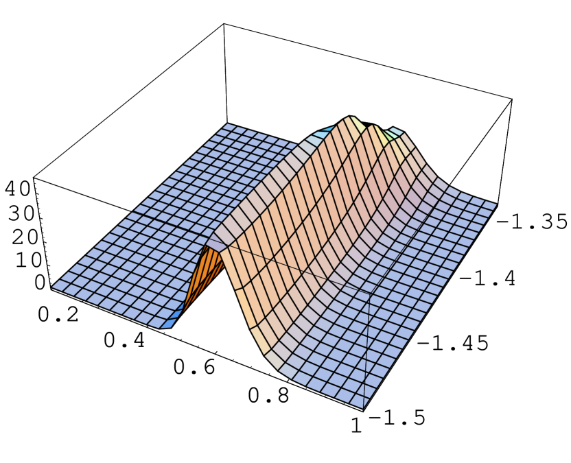
Figure 1: Two-dimensional probability distribution for $\omega$ and $h$.

Figure 2: Probability distribution for the parameter $\omega$.

Figure 3: Probability distribution for the parameter $h$.

Figure 4: Probability distribution for $\Omega_{m}$ and $h$ in the $\Lambda CDM$ model.

Figure 5: Probability distribution for $\Omega_{m}$ in the $\Lambda CDM$ model.

Figure 6: Probability distribution for $h$ in the $\Lambda CDM$ model.

The main quantity to be evaluated is the $\chi^{2}$ function, which gives the fitting quality:

$$\chi^{2}=\sum_{i=1}^{n}\frac{(\mu_{i0}^{t}-\mu_{i0}^{o})^{2}}{\sigma^{2}_{i}}\quad,$$ (29)

where $\mu_{i0}^{t}$ is the predicted theoretical value for the $ith$ supernova, $\mu_{i0}^{o}$ its observational value and $\sigma_{i}$ the error bar, taking already into account the effect of peculiar dispersion. From this quantity, a probability function is obtained:

$$P(\omega,h)=A\,e^{-\frac{\chi^{2}}{2}}\quad,$$ (30)

where $A$ is a normalization constant. The probability function for a unique parameter can be obtained by marginalizing on the remaining one:

$$P_{\omega}=\frac{\int P(\omega,h)dh}{\int\int P(\omega,h)dh\,d\omega}\quad,\quad P_{h}=\frac{\int P(\omega,h)d\omega}{\int\int P(\omega,h)dh\,d\omega}\quad.$$ (31)

In figures $1$, $2$ and $3$ the two dimensional probability distribution for $\omega$ and $h$, as well as the one-dimensional probability distribution for $\omega$ and $h$, in the Brans-Dicke flat model, are displayed. The most probable value for $\omega$ is $-1.5$, exactly the limiting case for the validity of solutions (8). However, $\omega=-1.5$ represents the case where the Brans-Dicke theory is conformally equivalent to the Einstein’s theory. Hence, the prediction should more properly stated by saying that the most probable value for the Brans-Dicke parameter is $\omega\rightarrow-1.5$. For $h$, the most probable value is $h=0.605$. The best fitting for the Brans-Dicke flat model is given by $\omega=-1.477$ and $h=0.594$, with $\chi^{2}=1.19318$.

In figures $4$, $5$ and $6$ the two-dimensional probability for $\Omega_{m}$ and $h$ and the one-dimensional probability function $\Omega_{m}$ and $h$, in the case of the $\Lambda CDM$ model, are displayed. For $h$, the prediction is quite similar to the Brans-Dicke case: the most probable value, marginalizing over $\Omega_{m}$, is $h=0.597$. The most probable value for the dark matter density parameter, marginalizing over $h$, is $\Omega_{m}=0.436$. The best fitting for the $\Lambda CDM$ model is given by $\Omega_{m}=0.506$ and $h=0.597$ with $\chi^{2}=1.19813$. The Brans-Dicke flat model gives a fitting slightly (but not negligible) better than the $\Lambda CDM$ model.

4 Conclusions

The general solutions for the Brans-Dicke flat cosmological model, determined by Gurevich et al, predict a late time accelerated universe for $-3/2<\omega<-4/3$, with an initial decelerated phase. This solution can be a candidate to describe the observed universe. In the present work, we have constrained this Brans-Dicke flat model using the supernovae type Ia ”gold sample”. We have compared the results with those obtained in a simplified $\Lambda CDM$ model. The Brans-Dicke model leads to a slightly smaller $\chi^{2}$ (which characterizes the quality of the fitting of the observational data) with respect to the $\Lambda CDM$ model.

In both models, the predicted value for the Hubble parameter $h$ is around $0.6$. This contrasts strongly with the estimation of $h$ coming from the anisotropy of the cosmic microwave background radiation, which leads to $h=0.72\pm 0.05$ [33]. However, this seems to be a general feature of the estimation of $h$ using supernovae data and CMB data [29]. For the Brans-Dicke model, the best value for the parameter $\omega$ is around $-1.5$. It must be remarked that the case $\omega=-1.5$ implies that the Brans-Dicke theory is conformally equivalent to general relativity. The minimum value for $\chi^{2}$ is obtained for $h=0.594$ and $\omega=-1.477$, with $\chi^{2}=1.19318$. In the $\Lambda CDM$ case, the best fitting is obtained with $\Omega_{m}=0.506$ and $h=0.597$, with $\chi^{2}=1.19813$

The results reported here indicate that, from the point of view of the supernovae type Ia data, the Brans-Dicke cosmological flat model leads to a quite viable scenario, even if the generalization to the non-flat cases should be made in order to have a more complete statistical analysis. However, at this point, this model must be seen as essentially a toy model, mainly due to the negative value for the parameter $\omega$. It would be interesting to connect the Brans-Dicke model exploited here with effective actions in four dimensions coming from M-theory and F-theory, which predict also a negative value for the parameter $\omega$.

The main problem with this scenario is that the values of $\omega$ are largely outside the values obtained with local tests, which indicate $\omega>1,000$ [13]. In reference [20], indications for a negative $\omega$ have also been obtained. Moreover, the range $-3/2<\omega<-4/3$ implies a negative gravitational coupling [28]. These drawbacks can be, in principle, circumvented if the gravitational coupling is scale-dependent, as suggested by considering quantum effects [16, 17]. In the present work, we made no attempt to reconcile the values for $\omega$ deduced from local tests with the corresponding values deduced from the analysis performed here. But, evidently, this problem must be addressed in order to have a complete realistic scenario.

One important point to be signed is that previous study indicate that structures can form in the Brans-Dicke model considered here during all the evolution of the universe, after the radiative phase, even the gravitational coupling is, at large scale, repulsive [34, 35]. However, a more detailed comparison between the theoretical predictions for matter agglomeration and the observational data must be made in order to constraint more strongly the model. In special, the possibility that the model can be unstable due to the repulsive gravitational coupling must be verified [36].
Acknowledgments: We thank Jérôme Martin for his remarks and criticisms. This work has been partially supported by CNPq (Brazil).

References

- [1] A.G. Riess et al, Astron. J. 116, 1009(1998)
- [2] S. Permultter et al, Astrophys. J. 517, 565(1998);
- [3] J.L. Tonry et al, Astrophys. J. 594, 1(2003);
- [4] A.G. Riess et al, Astrophys. J. 607, 665(2004);
- [5] V. Sahni,Dark Matter and Dark Energy, astro-ph/0403324;
- [6] I. Zlatev, L. Wang and P.J. Steinhardt, Phys. Rev. Lett. 82, 896(1999);
- [7] L. Wang, R.R. Caldwel, J.P. Ostriker and P.J. Steinhardt, Astrophys. J. 530, 17(2000);
- [8] Ph. Brax and J. Martin, Phys. Lett. B468, 45(1999);
- [9] C. Armendariz-Picon, V. Mukhanov, P.J. Steinhardt, Phys. Rev. D63, 103510(2001);
- [10] A. Yu. Kamenshchik, U. Moschella and V. Pasquier, Phys. Lett. B511, 265(2001);
- [11] J.C. Fabris, S.V.B. Gonçalves e P.E. de Souza, Gen. Rel. Grav. 34, 53(2002);
- [12] J.C. Fabris, S.V.B. Goncalves, R. de Sa Ribeiro, Bulk viscosity driving the acceleration of the universe, astro-ph/0503362, to appear in General Relativity and Gravitation;
- [13] C.M. Will, Living Rev. Rel. 4, 4(2001);
- [14] P.D. Mannheim, Found. of Phys. 30, 709(2000);
- [15] A. Barnaveli and M. Gogberashvili, Gen. Rel. Grav. 26, 1117(1994);
- [16] M. Reuter and H. Weyer, Phys. Rev. D70, 124028(2004);
- [17] I.L. Shapiro, J. Sola and H. Stefancic, JCAP 0501, 012(2005);
- [18] L.E. Gurevich, A.M. Finkelstein and V.A. Ruban, Astrophys. Spac. Sci. 22, 231(1973);
- [19] A.B. Batista, J.C. Fabris and R. de Sá Ribeiro, Gen. Rel. Grav. 33, 1237(2001);
- [20] O. Bertolami and P.J. Martins, Phys. Rev. D61, 064007(2000);
- [21] O. Arias, T. Gonzalez, Y. Leyva and I. Quirós, Class. Quant. Grav. 20, 2563(2003);
- [22] L. Amendola, Phys. Rev. Lett. 93, 181102(2004);
- [23] H. Kim, Phys. Lett. B606, 223(2005);
- [24] S. Carneiro, The cosmic coincidence in Brans-Dicke cosmologies, gr-qc/0505121;
- [25] A. Davidson, Class. Quant. Grav. 22, 1119(2005);
- [26] M.Arik and M.C.Calik, Can Brans-Dicke scalar field account for dark energy and dark matter?, gr-qc/0505035;
- [27] S. Das and N. Banerjee, An interacting scalar field and the recent cosmic acceleration, gr-qc/0507115;
- [28] S. Weinberg, Gravitation and cosmology, Wiley, New York(1972);
- [29] R. Colistete Jr. and J.C. Fabris, Class. Quant. Grav. 22, 2813(2005);
- [30] L. Amendola, S. Corasaniti and F. Occhionero, Time variability of the gravitational constant and type Ia supernovae, astro-ph/9907222;
- [31] E. Garcia-Berro, E. Gaztañaga, J. Isern, O. Benvenuto and L. Althaus, On the evolution of cosmological type Ia supernovae and the gravitational constant, astro-ph9907440;
- [32] A. Riazuelo and J-P. Uzan, Phys. Rev. D66, 023525(2002);
- [33] D.N. Spergel, Astrophys. J. Suppl. 148, 175(2003);
- [34] J.C. Fabris, A.B. Batista and J.P. Baptista, C.R. Acad. Sci. Paris 309, 791(1989);
- [35] J.P. Baptista, J.C. Fabris and S.V.B. Gonçalves, Astrophys. Spac. Sci. 246, 315(1996);
- [36] A.B. Batista, J.C. Fabris and S.V.G. Gonçalves, Class. Quant. Grav. 18, 1389(2001).