Forms of Eulerian correlation functions in the solar wind

Abstract

Current spacecraft missions such as Wind and ACE can be used to determine magnetic correlation functions in the solar wind. Data sets from these missions can, in principle, also be used to compute so-called Eulerian correlation functions. These temporal correlations are essential for understanding the dynamics of solar wind turbulence. In the current article we calculate these dynamical correlations by using well-established methods. These results are very useful for a comparison with Eulerian correlations obtained from space craft missions.

I Introduction

In the past idealized models for turbulent fluctuations which can be found in the solar wind plasma or in the interstellar medium have been proposed (e.g. Matthaeus et al. 1995). We are concerned with statistically axisymmetric models of magnetostatic fluctuations $\delta\vec{B}(\vec{x})$ that are transverse to a uniform mean magnetic field $\vec{B}_{0}$. If solar wind turbulence is considered, the mean field might be identified with the magnetic field of the Sun. The total magnetic field is a superposition of this mean field and the fluctuations $\vec{B}(\vec{x})=\vec{B}_{0}+\delta\vec{B}(\vec{x})$. Whereas we usually approximate the mean field by a constant field aligned parallel to the $z-$axis ($\vec{B}_{0}=B_{0}\vec{e}_{z}$), the turbulent contribution has to be replaced by turbulence models. Some prominant examples are slab, 2D, and two component models that include both slab and 2D contributions (e.g. Matthaeus et al. 1990).

There are recent spacecraft measurements of magnetic correlations in the solar wind (see e.g. Matthaeus et al. 2005, Dasso et al. 2007). Such measurements are very interesting and important since they allow an improved understanding of turbulence. For instance, characteristic length scales of turbulence such as the correlation length, the bendover scale, and the dissipation scale can be obtained from such observations. Also the investigation of spectral anisotropy by using data from different space craft missions such as Wind and ACE is possible. These properties of solar wind turbulence are very important for several investigations (heating and damping of the solar wind plasma, transport of charged cosmic rays). A further important turbulence property is the turbulence dynamics (the time dependence of the stochastic magnetic fields). In principle, data sets from Wind and ACE can also be used to compute dynamical correlation functions to explore the turbulence dynamics.

In a recent article (Shalchi 2008) magnetic correlation functions were computed analytically. Such analytical forms of magnetic correlations complement data analysis results such as Matthaeus et al. (2005) and Dasso et al. (2007). Since we expect that future data analysis work will also allow the investigation of temporal correlation functions, we explore theoretically (numerically and analytically) the forms of these Eulerian correlations. These results can be compared with data analysis results as soon as they are available.

The organization of the paper is as follows: in section 2 we define and discuss the basic parameters which are useful for describing turbulence. Furthermore, we explain the slab, the 2D, and the slab/2D compositel model. In section 3 we review different models for the turbulence dynamics. In section 4 we compute Eulerian correlation functions numerically and analytically. In section 5 the results of this article are summarized.

II General remarks - setting

II.1 The turbulence correlation function

The key function in turbulence theory is the two-point-two-time correlation tensor. For homogenous turbulence its components are

$$R_{lm}(\vec{x},t)=\left<\delta B_{l}(\vec{x},t)\delta B_{m}^{*}(\vec{0},0)\right>.$$ (1)

The brackets $\left<\dots\right>$ used here denote the ensemble average. It is convenient to introduce the correlation tensor in the $\vec{k}-$space. By using the Fourier representation

$$\delta B_{l}(\vec{x},t)=\int d^{3}k\;\delta B_{l}(\vec{k},t)e^{i\vec{k}\cdot\vec{x}}$$ (2)

we find

$$R_{lm}(\vec{x},t)=\int d^{3}k\int d^{3}k^{{}^{\prime}}\left<\delta B_{l}(\vec{k},t)\delta B_{m}^{*}(\vec{k}^{{}^{\prime}},0)\right>e^{i\vec{k}\cdot\vec{x}}.$$ (3)

For homogenous turbulence we have

$$\left<\delta B_{l}(\vec{k},t)\delta B_{m}^{*}(\vec{k}^{{}^{\prime}},0)\right>=P_{lm}(\vec{k},t)\delta(\vec{k}-\vec{k}^{{}^{\prime}})$$ (4)

with the correlation tensor in the $\vec{k}-$space $P_{lm}(\vec{k},t)$. By assuming the same temporal behaviour of all tensor components, we have

$$P_{lm}(\vec{k},t)=P_{lm}(\vec{k})\;\Gamma(\vec{k},t)$$ (5)

with the dynamical correlation funtion $\Gamma(\vec{k},t)$. Eq. (3) becomes than

$$R_{lm}(\vec{x},t)=\int d^{3}k\;P_{lm}(\vec{k})\Gamma(\vec{k},t)e^{i\vec{k}\cdot(\vec{x})}$$ (6)

with the magnetostatic tensor $P_{lm}(\vec{k})=\left<\delta B_{l}(\vec{k})\delta B_{m}^{*}(\vec{k})\right>$.

II.2 The two-component turbulence model

In this paragraph we discuss the static tensor $P_{lm}(\vec{k})$ defined in Eq. (6). Matthaeus & Smith (1981) have investigated axisymmetric turbulence and derived a general form of $P_{lm}(\vec{k})$ for this special case. In our case the symmetry-axis has to be identified with the axis of the uniform mean magnetic field $\vec{B}_{0}=B_{0}\vec{e}_{z}$. For most applications (e.g. plasma containment devices, interplanetary medium) the condition of axisymmetry should be well satisfied. Furthermore, we neglect magnetic helicity and we assume that the parallel component of the turbulent fields is zero or negligible small ($\delta B_{z}=0$). In this case the correlation tensor has the form

$$P_{lm}(\vec{k})=A(k_{\parallel},k_{\perp})\left[\delta_{lm}-\frac{k_{l}k_{m}}{k^{2}}\right],\quad l,m=x,y$$ (7)

and $P_{lz}=P_{zm}=0$. The function $A(k_{\parallel},k_{\perp})$ is controlled by two turbulence properties: the turbulence geometry and the turbulence wave spectrum. The geometry describes how $A(k_{\parallel},k_{\perp})$ depends on the direction of the wave vector $\vec{k}$ with respect to the mean field. There are at least three established models for the turbulence geometry:

1. The slab model: here we assume the form

   $$A^{slab}(k_{\parallel},k_{\perp})=g^{slab}(k_{\parallel})\frac{\delta(k_{\perp})}{k_{\perp}}.$$ (8)

   In this model the wave vectors are aligned parallel to the mean field ($\vec{k}\parallel\vec{B}_{0}$).

2. The 2D model: here we replace $A(k_{\parallel},k_{\perp})$ by

   $$A^{2D}(k_{\parallel},k_{\perp})=g^{2D}(k_{\perp})\frac{\delta(k_{\parallel})}{k_{\perp}}.$$ (9)

   In this model the wave vectors are aligned perpendicular to the mean field ($\vec{k}\perp\vec{B}_{0}$) and are therefore in a two-dimensional (2D) plane.

3. The slab/2D composite (or two-component) model: In reality the turbulent fields can depend on all three coordinates of space. A quasi-three-dimensional model is the so-called slab/2D composite model, where we assume a superposition of slab and 2D fluctuations: $\delta B_{i}^{comp}(x,y,z)=\delta B_{i}^{slab}(z)+\delta B_{i}^{2D}(x,y)$. Because of $<\delta B_{i}^{slab}(z)\delta B_{j}^{*,2D}(x,y)>=0$, the correlation tensor has the form

   $$P_{lm}^{comp}(\vec{k})=P_{lm}^{slab}(\vec{k})+P_{lm}^{2D}(\vec{k}).$$ (10)

   In the composite model the total strength of the fluctuations is $\delta B^{2}=\delta B_{slab}^{2}+\delta B_{2D}^{2}$. The composite model is often used to model solar wind turbulence. It was demonstrated by several authors (e.g. Bieber et al. 1994, 1996) that $20\%$ slab / $80\%$ 2D should be realistic in the solar wind at 1 AU heliocentric distance.

The wave spectrum describes the wave number dependence of $A(k_{\parallel},k_{\perp})$. In the slab model the spectrum is described by the function $g^{slab}(k_{\parallel})$ and in the 2D model by $g^{2D}(k_{\perp})$.

As demonstrated in Shalchi (2008), the combined correlation functions (defined as $R_{\perp}=R_{xx}+R_{yy}$) for pure slab turbulence is given by

$$R_{\perp}^{slab}(z)=8\pi\int_{0}^{\infty}dk_{\parallel}\;g^{slab}(k_{\parallel})\cos(k_{\parallel}z)$$ (11)

and the correlation function for pure 2D is

$$R_{\perp}^{2D}(\rho)=2\pi\int_{0}^{\infty}dk_{\perp}\;g^{2D}(k_{\perp})J_{0}(k_{\perp}\rho).$$ (12)

Here $z$ is the distance parallel with respect to the mean magnetic field and $\rho$ denotes the distance in the perpendicular direction. To evaluate these formulas we have to specify the two wave spectra $g^{slab}(k_{\parallel})$ and $g^{2D}(k_{\perp})$.

II.3 The turbulence spectrum

In a cosmic ray propagation study, Bieber et al. (1994) proposed spectra of the form

$$g^{slab}(k_{\parallel}) = \frac{C(\nu)}{2\pi}l_{slab}\delta B_{slab}^{2}(1+k_{\parallel}^{2}l_{slab}^{2})^{-\nu}$$

$$g^{2D}(k_{\perp}) = \frac{2C(\nu)}{\pi}l_{2D}\delta B_{2D}^{2}(1+k_{\perp}^{2}l_{2D}^{2})^{-\nu}$$ (13)

with the inertial range spectral index $2\nu$, the two bendover length scales $l_{slab}$ and $l_{2D}$, and the strength of the slab and the 2D fluctuations $\delta B_{slab}^{2}$ and $\delta B_{2D}^{2}$. By requiring normalization of the spectra

$$\delta B^{2}=\delta B_{x}^{2}+\delta B_{y}^{2}+\delta B_{z}^{2}=\int d^{3}k\;\left[P_{xx}(\vec{k})+P_{yy}(\vec{k})+P_{zz}(\vec{k})\right]$$ (14)

we find

$$C(\nu)=\frac{1}{2\sqrt{\pi}}\frac{\Gamma(\nu)}{\Gamma(\nu-1/2)}.$$ (15)

By combining these spectra with Eqs. (11) and (12) the slab correlation function

$$R_{\perp}^{slab}(z)=4C(\nu)\delta B_{slab}^{2}l_{slab}\int_{0}^{\infty}dk_{\parallel}\;(1+k_{\parallel}^{2}l_{slab}^{2})^{-\nu}\cos(k_{\parallel}z)$$ (16)

as well as the 2D correlation function

$$R_{\perp}^{2D}(\rho)=4C(\nu)\delta B_{2D}^{2}l_{2D}\int_{0}^{\infty}dk_{\perp}\;(1+k_{\perp}^{2}l_{2D}^{2})^{-\nu}J_{0}(k_{\perp}\rho)$$ (17)

can be calculated. In Eq. (17) we have used the Bessel function $J_{0}(x)$. In Shalchi (2008) such calculations valid for magnetostatic turbulence are presented.

II.4 Correlation functions for dynamical turbulence

For dynamical turbulence the slab and the 2D correlation functions from Eqs. (11) and (12) become

$$R_{\perp}^{slab}(z) = 8\pi\int_{0}^{\infty}dk_{\parallel}\;g^{slab}(k_{\parallel})\cos(k_{\parallel}z)\Gamma^{slab}(k_{\parallel},t)$$

$$R_{\perp}^{2D}(\rho) = 2\pi\int_{0}^{\infty}dk_{\perp}\;g^{2D}(k_{\perp})J_{0}(k_{\perp}\rho)\Gamma^{2D}(k_{\perp},t).$$ (18)

For the model spectrum defined in the previous paragraph these formulas become

$$R_{\perp}^{slab}(z,t) = 4C(\nu)\delta B_{slab}^{2}l_{slab}\int_{0}^{\infty}dk_{\parallel}\;(1+k_{\parallel}^{2}l_{slab}^{2})^{-\nu}\cos(k_{\parallel}z)\;\Gamma^{slab}(k_{\parallel},t)$$

$$R_{\perp}^{2D}(\rho,t) = 4C(\nu)\delta B_{2D}^{2}l_{2D}\int_{0}^{\infty}dk_{\perp}\;(1+k_{\perp}^{2}l_{2D}^{2})^{-\nu}J_{0}(k_{\perp}\rho)\;\Gamma^{2D}(k_{\perp},t).$$ (19)

To evaluate these equations we have to specify the dynamical correlation functions $\Gamma^{slab}(k_{\parallel},t)$ and $\Gamma^{2D}(k_{\perp},t)$ which is done in the next section.

III Dynamical turbulence and plasma wave propagation effects

In the following, we discuss several models for the dynamical correlation function $\Gamma(\vec{k},t)$. In Table 1, different models for the dynamical correlation function are summarized and compared with each other.

Model	$\Gamma^{slab}(k_{\parallel},t)$	$\Gamma^{2D}(k_{\perp},t)$
Magnetostatic model	$1$	$1$
Damping model of dynamical turbulence	$e^{-\alpha v_{A}k_{\parallel}t}$	$e^{-\alpha v_{A}k_{\perp}t}$
Random sweeping model	$e^{-(\alpha v_{A}k_{\parallel}t)^{2}}$	$e^{-(\alpha v_{A}k_{\perp}t)^{2}}$
Undampled shear Alfvén waves	$\cos(\pm v_{A}k_{\parallel}t)$	$1$
Undampled fast mode waves	$\cos(v_{A}k_{\parallel}t)$	$\cos(v_{A}k_{\perp}t)$
NADT model	$\cos(\pm v_{A}k_{\parallel}t)e^{-\gamma_{slab}t}$	$e^{-\gamma_{2D}t}$

Table 1: Different models for the dynamical correlation function $\Gamma(\vec{k},t)$. Here, $v_{A}$ is the Alfvén speed and $\alpha$ is a parameter that allows to adjust the strength of dynamical effects. The parameters $\gamma_{slab}$ and $\gamma^{2D}$ of the NADT model are defined in Eq. (26).

In the $\vec{k}-$space these models show a very different decorrelation in time. In the Section IV we compute the dynamical correlation functions in the configuration space for these different models

III.1 Damping and random sweeping models

One of the first authors discussing dynamical turbulence were Bieber et al. (1994). In their article, the authors proposed two models for the dynamical correlation function:

$$\Gamma_{DT}(\vec{k},t) = e^{-t/t_{c}(\vec{k})}\quad\textnormal{(damping model of dynamical turbulence)}$$

$$\Gamma_{RS}(\vec{k},t) = e^{-(t/t_{c}(\vec{k}))^{2}}\quad\textnormal{(random sweeping model)}$$ (20)

with the correlation time scale $t_{c}(\vec{k})$. Bieber et al. (1994) estimated the correlation time as

$$\frac{1}{t_{c}(\vec{k})}=\alpha v_{A}\mid\vec{k}\mid.$$ (21)

Here, $v_{A}$ is the Alfvén speed and $\alpha$ is a parameter which allows to adjust the strength of the dynamical effects, ranging from $\alpha=0$ (magnetostatic turbulence) to $\alpha=1$ (strongly dynamical turbulence). Bieber et al. (1994) also suggested that the parameter $\alpha$ could be interpreted as $\delta B/B_{0}$. In this case, the correlation time scale $t_{c}(\vec{k})$ becomes comparable to the eddy turnover time. Also, decorrelation effects related to plasma waves (see, e.g., Schlickeiser & Achatz 1993) can be achieved by expressing $\alpha$ through parameters such as the plasma $\beta$ (for a definition see also Schlickeiser & Achatz 1993). The damping model was originally introduced for a particle scattering study in dynamcial turbulence by Bieber et al. (1994). In this model, the dynamical correlation function has an exponential form, whereas in the random sweeping model $\Gamma(\vec{k},t)$ has a Gaussian form.

III.2 Plasma wave turbulence

Another prominent model is the plasma wave model which is discussed in Schlickeiser (2002). In this model, the dynamical correlation function has the form

$$\Gamma_{PW}(\vec{k},t)=\cos(\omega t)e^{-\gamma t}.$$ (22)

Here, $\omega$ is the plasma wave dispersion relation, whereas $\gamma$ desribes plasma wave damping. Often, undamped plasma waves are considered, where $\Gamma_{PW}(\vec{k},t)=\cos(\omega t)$ and the dynamical correlation function is a purely oszillating function. Prominent examples for different plasma waves are Shear Alfvén waves, where $\omega=\pm v_{A}k_{\parallel}$, and fast magnetosonic waves, where $\omega=v_{A}k$.

III.3 The nonlinear anisotropic dynamical turbulence model

Recently, an improved dynamical turbulence model, namely the nonlinear anisotropic dynamical turbulence (NADT) model, has been proposed by Shalchi et al. (2006). This model takes into account plasma wave propagation effects as well as dynamical turbulence effects. The NADT model was formulated for the slab/2D composite model, where, in general, we have the two different dynamical correlation functions $\Gamma^{slab}(k_{\parallel},t)$ and $\Gamma^{2D}(k_{\perp},t)$, namely

$$\Gamma^{slab}(k_{\parallel},t) = \cos(\omega t)e^{-\gamma^{slab}\;t}$$

$$\Gamma^{2D}(k_{\perp},t) = e^{-\gamma^{2D}\;t}$$ (23)

with

$$\gamma^{slab} = \beta$$

$$\gamma^{2D} = \beta\;\left\{\begin{array}[]{ccc}1&\textnormal{for}&k_{\perp}l_{2D}\leq 1\\ (k_{\perp}l_{2D})^{2/3}&\textnormal{for}&k_{\perp}l_{2D}\geq 1.\end{array}\right.$$ (26)

and with the plasma wave dispersion relation of shear Alfvén waves

$$\omega=jv_{A}k_{\parallel}\quad j=\pm 1.$$ (27)

In Eq. (26) the parameter $\beta$ can be expressed by the strength of the 2D component $\delta B_{2D}/B_{0}$, the 2D bendover scale $l_{2D}$, and the Alfvén Speed $v_{A}$ (see Shalchi et al. 2006):

$$\beta=\sqrt{2}\frac{v_{A}}{l_{2D}}\frac{\delta B_{2D}}{B_{0}}.$$ (28)

These forms of the temporal correlation function are discussed in more detail in Shalchi et al. (2006). They are based on the work of Shebalin (1983), Matthaeus et al. (1990), Tu & Marsch (1993), Oughton et al. (1994), Zhou et al. (2004), Oughton et al. (2006). In the current article we approximate $\gamma^{2D}$ in Eq. (26) by

$$\gamma^{2D}=\beta\left(1+k_{\perp}l_{2D}\right)^{2/3}$$ (29)

for simplicity.

The parameter $j$ in Eq. (27) is used to track the wave propagation direction ($j=+1$ is used for forward and $j=-1$ for backward to the ambient magnetic field propagating Alfvén waves). A lot of studies have addressed the direction of propagation of Alfvénic turbulence, see, for instance, Bavassano (2003). In general, one would expect that, closer to the sun, most waves should propagate forward and, far away from the sun, the wave intensities should be equal for both directions. Most of the observations, which allow conclusions on space plasma and particle propagation properties, have been performed in the solar wind at 1 AU heliocentric distance. Thus, we can assume that all waves propagate forward, and we therefore set $j=+1$ in the current article.

IV Eulerian correlation functions

To investigate the different models we calculate the (combined) single-point-two-time correlation function defined by

$$E_{\perp}(t):=R_{\perp}(\vec{x}=0,t)=\left<\delta B_{l}(0,t)\delta B_{m}^{*}(0,0)\right>.$$ (30)

Since this function is of particular importance in understanding dynamical turbulence effects and interactions with energetic charged particles this function is also known as Eulerian correlation function $E_{\perp}(t)$. For the different models discussed in Section III, Eqs. (19) become

$$E_{\perp}^{slab}(t) = 4C(\nu)\delta B_{slab}^{2}\int_{0}^{\infty}dx\;(1+x^{2})^{-\nu}$$ (36)

$$\times \left\{\begin{array}[]{cc}1&\textnormal{magnetostatic model}\\ \cos(\tau x)&\textnormal{Alfv\'{e}n waves}\\ e^{-\alpha\tau x}&\textnormal{damping model}\\ e^{-(\alpha\tau x)^{2}}&\textnormal{random sweeping model}\\ \cos(\tau x)e^{-\xi\tau}&\textnormal{NADT model}\end{array}\right.$$

and

$$E_{\perp}^{2D}(t) = 4C(\nu)\delta B_{2D}^{2}\int_{0}^{\infty}dx\;(1+x^{2})^{-\nu}$$ (42)

$$\times \left\{\begin{array}[]{cc}1&\textnormal{magnetostatic model}\\ 1&\textnormal{Alfv\'{e}n waves}\\ e^{-\alpha\frac{l_{slab}}{l_{2D}}\tau x}&\textnormal{damping model}\\ e^{-(\alpha\frac{l_{slab}}{l_{2D}}\tau x)^{2}}&\textnormal{random sweeping model}\\ e^{-\xi\tau(1+x)^{2/3}}&\textnormal{NADT model}\end{array}\right.$$

Here we have used the integral transformations $x=k_{\parallel}l_{slab}$ and $x=k_{\perp}l_{2D}$. Furthermore we used the dimensionless time

$$\tau=v_{A}t/l_{slab}$$ (43)

and the parameter

$$\xi=\sqrt{2}\frac{\delta B_{2D}}{B_{0}}\frac{l_{slab}}{l_{2D}}.$$ (44)

In the following paragraphs we evaluate Eqs. (36) and (42) numerically and analytically.

IV.1 Numerical calculation of Eulerian correlations

In Figs. 1 and 2 the results for the slab correlation function and in Figs. 3 and 4 for the 2D correlation function are shown for the different dynamical turbulence models. To obtain these figures we have solved the integrals in Eqs. (36) and (42) numerically. For the damping model and the random sweeping model we used $\alpha=1$. Furthermore, we used $l_{2D}=0.1l_{slab}$ as in previous articles based on the result of laboratory experiments such as Robinson & Rusbridge (1971). For the turbulence spectrum in the inertial range we employ a Kolmogorov (1941) behavior by setting $\nu=5/6$.

As shown in Figs. 1 - 4, the Eulerian correlations obtained for the damping model and the random sweeping model are very similar. The results obtained by employing the NADT model are, however, quite different from the other models.

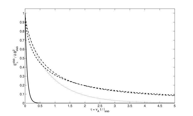
Figure 1: The slab correlation function $R_{\perp}^{slab}(0,t)/\delta B_{slab}^{2}$ as a function of the time $\tau=v_{A}t/l_{slab}$. Shown are the results obtained for the Alfvénic plasma wave model (dotted line), the damping model of dynamical turbulence (dashed line), the random sweeping model (dash-dotted line), and the NADT model (solid line).

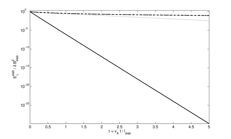
Figure 2: Same caption as in Fig. 1 but now as semi-log-plot. Clearly we can see that we find an exponential function for the Eulerian correlation if we employ the Alfv́en wave model (dotted line) or the NADT model (solid line).

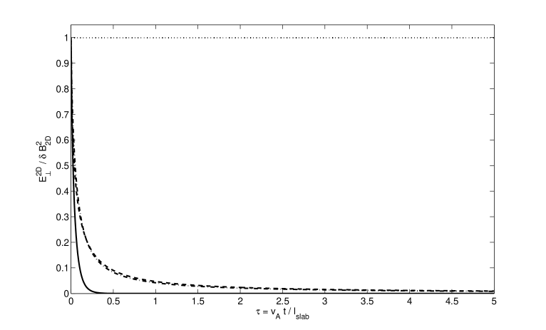
Figure 3: The 2D correlation function $R_{\perp}^{2D}(0,t)/\delta B_{2D}^{2}$ as a function of the time $\tau=v_{A}t/l_{slab}$. Shown are the results obtained for the Alfvénic plasma wave model (dotted line), the damping model of dynamical turbulence (dashed line), the random sweeping model (dash-dotted line), and the NADT model (solid line). The result for undampled Alfvén waves corresponds to the magnetostatic model.

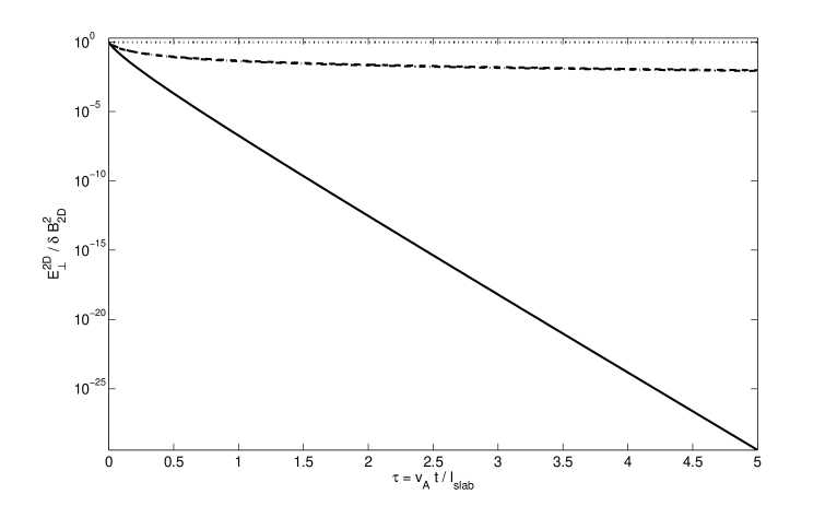
Figure 4: Same caption as in Fig. 3 but now as semi-log-plot. Clearly we can see that we find an exponential function for the Eulerian correlation if we employ the NADT model (solid line).

IV.2 Analytical calculation of Eulerian correlations

Here we compute analytically the different Eulerian correlations. For magnetostatic (MS) turbulence we can use

$$\int_{0}^{\infty}dx\;(1+x^{2})^{-\nu}=\frac{1}{4C(\nu)}$$ (45)

and therefore

$$E_{\perp}^{slab,MS} = \delta B_{slab}^{2}$$

$$E_{\perp}^{2D,MS} = \delta B_{2D}^{2}$$ (46)

which is the expected result. In the following paragraphs we investigate the different other turbulence models.

IV.2.1 Undampled shear Alfvén waves

In this case we can use (see, e.g., Shalchi 2008)

$$\int_{0}^{\infty}dx\;(1+x^{2})^{-\nu}\cos(\tau x)=\frac{1}{\Gamma(\nu)}\left(\frac{2}{\tau}\right)^{1/2-\nu}K_{1/2-\nu}(\tau)$$ (47)

to derive

$$E_{\perp}^{slab,Alf}(t)=\frac{4\delta B_{slab}^{2}}{\Gamma(\nu-1/2)}\left(\frac{2l_{slab}}{v_{A}t}\right)^{1/2-\nu}K_{1/2-\nu}\left(\frac{v_{A}t}{l_{slab}}\right).$$ (48)

Obviously the characteristic time scale for temporal decorrelation $t_{c}$ is

$$t_{c}^{slab,Alf}=\frac{l_{slab}}{v_{A}}.$$ (49)

Following Shalchi (2008), the Modified Bessel function in Eqs. (47) and (48) can be approximated for large arguments. We find for times much larger than the temporal decorrelation time

$$E_{\perp}^{slab,Alf}(t\gg t_{c})\approx\frac{2\sqrt{\pi}}{\Gamma(\nu-1/2)}\delta B_{slab}^{2}\left(\frac{2l_{slab}}{v_{A}t}\right)^{1-\nu}e^{-v_{A}t/l_{slab}}.$$ (50)

For the special case $\nu=1$ we obtain an exponential function. For the 2D Eulerian correlations we always have $E_{\perp}^{2D,Alf}(t)=\delta B_{2D}^{2}$, since there are no wave propagation effects in the perpendicular direction for (undamped) Alfvénic plasma waves.

IV.2.2 Damping model of dynamical turbulence

For the damping model of dynamical turbulence (DT) the integrals in Eqs. (36) and (42) are difficult to solve. The results can be found in the appendix. As shown there, the characteristic time scale for the temporal decorrelation is

$$t_{c}^{DT}=\left\{\begin{array}[]{cc}\frac{l_{slab}}{\alpha v_{A}}&\textnormal{for slab fluctuations}\\ \frac{l_{2D}}{\alpha v_{A}}&\textnormal{for 2D fluctuations}\end{array}\right.$$ (53)

For the case $t\gg t_{c}$ corresponding to $a_{i}\tau\gg 1$ ($i=slab,2D$) with

$$a_{slab} = \alpha$$

$$a_{2D} = \alpha\frac{l_{slab}}{l_{2D}}$$ (54)

we can easily compute the Eulerian correlation function approximatelly. For large $a_{i}\tau$ there is only a contribution to the exponential function in Eqs. (36) and (42) for $x\rightarrow 0$. Thus, we can approximate

$$\int_{0}^{\infty}dx\;(1+x^{2})^{-\nu}e^{-a_{i}\tau x}\approx\int_{0}^{\infty}dx\;e^{-a_{i}\tau x}=\frac{1}{a_{i}\tau}$$ (55)

to obtain

$$E_{\perp}^{DT}(t\gg t_{c})=\frac{4C(\nu)}{\alpha v_{A}t}\left\{\begin{array}[]{cc}\delta B_{slab}^{2}l_{slab}&\textnormal{for slab fluctuations}\\ \delta B_{2D}^{2}l_{2D}&\textnormal{for 2D fluctuations}.\end{array}\right.$$ (58)

For the damping model of dynamical turbulence the Eulerian correlation function tends to zero with $E_{\perp}^{DT}\sim t^{-1}$.

IV.2.3 Random sweeping model

For the random sweeping model the analytical results can also be found in the appendix. As shown there we find the same temporal correlation time scale $t_{c}$ as for the damping model of dynamical turbulence (see Eq. (53)). For time scale satisfying $t\gg t_{c}$ we can use

$$\int_{0}^{\infty}dx\;(1+x^{2})^{-\nu}e^{-(a_{i}\tau x)^{2}}\approx\int_{0}^{\infty}dx\;e^{-(a_{i}\tau x)^{2}}=\frac{\sqrt{\pi}}{2a_{i}\tau}$$ (59)

to find

$$E_{\perp}^{RS}(t\gg t_{c})=2\sqrt{\pi}C(\nu)\left\{\begin{array}[]{cc}\delta B_{slab}^{2}\frac{l_{slab}}{\alpha v_{A}t}&\textnormal{for slab fluctuations}\\ \delta B_{2D}^{2}\frac{l_{2D}}{\alpha v_{A}t}&\textnormal{for 2D fluctuations}.\end{array}\right.$$ (62)

Obviously the results for the random sweeping model are very similar to the results obtained for the damping model. This conclusion based on analytical investigations agrees with the numerical results from Figs. 1 - 4.

IV.2.4 NADT model

Here we have to distinguish between the slab and the 2D correlation function. For the slab function we can use the result for Alfvén waves with an additional factor $exp(-\xi\tau)$. Therefore, we find for late times

$$E_{\perp}^{slab,NADT}(t\gg t_{c})\approx\frac{2\sqrt{\pi}}{\Gamma(\nu-1/2)}\delta B_{slab}^{2}\left(\frac{2l_{slab}}{v_{A}t}\right)^{1-\nu}e^{-v_{A}t(1+\xi)/l_{slab}}.$$ (63)

In this case there are two correlation time scales. The first is associated with the plasma wave (PW) propagation effects

$$t_{c,PW}^{slab,NADT}=\frac{l_{slab}}{v_{A}}$$ (64)

and the second is associated with the dynamical turbulence (DT) effects. The latter correlation time is

$$t_{c,DT}^{NADT}=\frac{l_{slab}}{v_{A}\xi}=\frac{1}{\sqrt{2}}\frac{B_{0}}{\delta B_{2D}}\frac{l_{2D}}{v_{A}}.$$ (65)

For the 2D fluctuations the situation is more complicated and, thus, the analytical calculations can be found in the appendix. As demonstrated there the correlation time scale is given by Eq. (65). The behavior of the Eulerian correlation function for late time ($t\gg t_{c,DT}^{NADT}$) is an exponential function

$$E_{\perp}^{2D}\approx 4C(\nu)\delta B_{2D}^{2}e^{-v_{A}t\xi/l_{slab}}.$$ (66)

This exponential result agrees with our numerical findings visualized in Figs. 3 and 4.

V Summary and conclusion

In this article we have calculated and discussed Eulerian correlation functions. The motivation for this work are recent articles from Matthaeus et al. (2005) and Dasso et al. (2007). In these papers it was demonstrated, that magnetic correlation functions can be obtain from spacecrafts measurements (ACE and Wind). We expect that from such observations also Eulerian correlations can be obtained. In the current article we computed analytically and numerically these correlations. These theoretical results are very useful for a comparison with data obtained from ACE and Wind.

We have employed several standard models for solar wind turbulence dynamics, namely the (undamped and Alfvénic) plasma wave model, the damping model of dynamical turbulence, the random sweeping model, and the nonlinear anisotropic dynamical turbulence (NADT) model. All these model are combined with a two-component model and a standard form of the turbulence wave spectrum. As shown, we find very similar Eulerian correlations for the damping model and the random sweeping model. Therefore, we expect that in a comparison between these models and spacecraft data, one can not decide which of these models is more realistic. The NADT model presented in Shalchi et al. (2006), however, provides different results in comparison to these previous models. In table 2 we have compared the different correlation time scale derived in this article for the different models.

Model	$t_{c}^{slab}$	$t_{c}^{2D}$
Magnetostatic model	$\infty$	$\infty$
Undampled shear Alfvén waves	$\frac{l_{slab}}{v_{A}}$	$\infty$
Damping model of dynamical turbulence	$\frac{l_{slab}}{\alpha v_{A}}$	$\frac{l_{2D}}{\alpha v_{A}}$
Random sweeping model	$\frac{l_{slab}}{\alpha v_{A}}$	$\frac{l_{2D}}{\alpha v_{A}}$
NADT model (plasma wave effects)	$\frac{l_{slab}}{v_{A}}$	no effect
NADT model (dyn. turbulence effects)	$\frac{1}{\sqrt{2}}\frac{B_{0}}{\delta B_{2D}}\frac{l_{2D}}{v_{A}}$	$\frac{1}{\sqrt{2}}\frac{B_{0}}{\delta B_{2D}}\frac{l_{2D}}{v_{A}}$

Table 2: Comparison for the different correlation time scale found in this article. For the damping model of dynamical turbulence and the random sweeping model we found the same correlation times. For the NADT model there are two correlation times, one scale for the plasma wave propagation effects and one scale for the dynamical turbulence effects.

By comparing the results of this article with spacecraft measurements, we can find out whether modern models like the NADT model is realistic or not. This would be very useful for testing our understanding of turbulence. Some results of this article, such as Eqs. (18) are quite general and can easily be applied for other turbulence models (e.g. other wave spectra).

Appendix A Exact analytical forms of Eulerian correlation functions

By using Abramowitz & Stegun (1974) and Gradshteyn & Ryzhik (2000) we can compute analytically the different Eulerian correlation functions defined in Eqs. (36) and (42). For the plasma wave model the results are given in the main part of the paper.

A.1 Damping model of dynamical turbulence

For the damping model of dynamical turbulence we can use

$$\int_{0}^{\infty}dx\;(1+x^{2})^{-\nu}e^{-a_{i}\tau x} = \frac{2^{-1/2-\nu}\pi^{3/2}(a_{i}\tau)^{\nu-1/2}}{\Gamma(\nu)}$$ (67)

$$\times \left[2J_{\nu-1/2}(a_{i}\tau)Csc(2\pi\nu)-J_{1/2-\nu}(a_{i}\tau)Sec(\pi\nu)+Csc(\pi\nu)H_{1/2-\nu}(a_{i}\tau)\right].$$

Here we used Bessel functions $J_{n}(z)$ and the Struve function $H_{n}(z)$. By making use of this result we find for the Eulerian correlation function

$$E_{\perp}^{i,DT}(t) = 4C(\nu)\delta B_{i}^{2}\frac{2^{-1/2-\nu}\pi^{3/2}(a_{i}\tau)^{\nu-1/2}}{\Gamma(\nu)}$$ (68)

$$\times \left[2J_{\nu-1/2}(a_{i}\tau)Csc(2\pi\nu)-J_{1/2-\nu}(a_{i}\tau)Sec(\pi\nu)+Csc(\pi\nu)H_{1/2-\nu}(a_{i}\tau)\right]$$

with $i=slab,2D$ and

$$a_{slab} = \alpha$$

$$a_{2D} = \alpha\frac{l_{slab}}{l_{2D}}$$ (69)

for the damping model of dynamical turbulence.

A.2 Random sweeping model

For the random sweeping model we can employ

$$\int_{0}^{\infty}dx\;(1+x^{2})^{-\nu}e^{-(a_{i}\tau x)^{2}}=\frac{\sqrt{\pi}}{2}U\left(\frac{1}{2},\frac{3}{2}-\nu,a_{i}^{2}\tau^{2}\right)$$ (70)

with the confluent hypergeometric function $U(a,b,z)$. By employing this result we find for the Eulerian correlation function

$$E_{\perp}^{i,RS}(t)=2\sqrt{\pi}C(\nu)\delta B_{i}^{2}U\left(\frac{1}{2},\frac{3}{2}-\nu,a_{i}^{2}\tau^{2}\right)$$ (71)

for the random sweeping model.

A.3 NADT model

For the NADT model we only have to explore the 2D fluctuations (the slab result is trivial and discussed in the main part of the this paper). Eq. (42) can be rewritten as

$$E_{\perp}^{2D}=4C(\nu)\delta B_{2D}^{2}\left[\int_{0}^{1}dx\;e^{-\xi\tau}+\int_{1}^{\infty}dx\;x^{-2\nu}e^{-\xi\tau x^{2/3}}\right]$$ (72)

The first integral in trivial, the second one can be expressed by an exponential integral function $E_{\mu}(z)$:

$$E_{\perp}^{2D}=4C(\nu)\delta B_{2D}^{2}\left[e^{-\xi\tau}+\frac{3}{2}E_{3\nu-1/2}(\xi\tau)\right].$$ (73)

This is the final result for the Eulerian correlation function of the 2D fluctuations. To evaluate this expression for late times ($\xi\tau\gg 1$) we can approximate the exponential integral function by using

$$E_{3\nu-1/2}(\xi\tau\gg 1)\approx\int_{1}^{\infty}e^{-\xi\tau x}=\frac{e^{-\xi\tau}}{\xi\tau}.$$ (74)

Here we assumed that the main contribution to the integral comes from the smallest values of $x$, namely $x\approx 1$. By combining Eq. (74) with Eq. (73) we find approximatelly

$$E_{\perp}^{2D}\approx 4C(\nu)\delta B_{2D}^{2}e^{-\xi\tau}$$ (75)

corresponding to an exponential behavior of the Eulerian correlation function. For the correlation time scale we find $\tau_{c}=1/\xi$. A further discussion of these results can be found in the main part of the text.

References

- (1) Abramowitz, M. & Stegun, I. A., Handbook of Mathematical Functions, (Dover Publications, New York, 1974)
- (2) Bavassano, B., 2003, AIP Conference Proceedings, 679, 377
- (3) Bieber, J. W., Matthaeus, W. H., Smith, C. W., Wanner, W., Kallenrode, M.-B. & Wibberenz, G., 1994, The Astrophysical Journal, 420, 294
- (4) Bieber, J. W., Wanner, W. & Matthaeus, W. H., 1996, Journal of Geophysical Research, 101, 2511
- (5) Dasso, S., Matthaeus, W. H., Weygand, J. M., Chuychai, P., Milano, L. J., Smith, C. W. & Kivelson, M. G., ICRC (2007)
- (6) Gradshteyn, I. S. & Ryzhik, I. M., Table of integrals, series, and products, Academic Press, New York, 2000
- (7) Kolmogorov, A. N., 1941, Dokl. Akad. Nauk. SSSR, 30, 301
- (8) Matthaeus, W. H. & Smith, C., 1981, Physical Review A - General Physics, 24, 2135
- (9) Matthaeus, W. H. & Goldstein, M. L., and Roberts, D. A., 1990, Journal of Geophysical Research, 95, 20673
- (10) Matthaeus, W. H., Gray, P. C., Pontius, D. H. Jr. & Bieber, J. W., Phys. Rev. Lett., 75, 2136 (1995)
- (11) Matthaeus, W. H., Dasso, S., Weygand, J. M., Milano, L. J., Smith, C. W. & Kivelson, M. G., Phys. Rev. Lett., 95, 23 (2005)
- (12) Oughton, S., Priest, E. & Matthaeus W. H., 1994, J. Fluid Mech., 280, 95
- (13) Oughton, S., Dmitruk, P. & Matthaeus, W. H., 2006, Physics of Plasmas 13, 042306
- (14) Robinson, D. C. & Rusbridge, M. G., 1971, Phys. Fluids, 14, 2499
- (15) Schlickeiser, R. & Achatz, U., 1993, Journal of Plasma Physics, 49, 63
- (16) Schlickeiser, R., Cosmic Ray Astrophysics, Springer-Verlag, Berlin, 2002
- (17) Shalchi, A., Bieber, J. W., Matthaeus, W. H. & Schlickeiser, R., 2006, The Astrophysical Journal, 642, 230
- (18) Shalchi, A., 2008, Astrophysics and Space Science, 315, 31
- (19) Shebalin, J. V., Matthaeus, W. H. & Montgomery, D.,1983, J. Plasma Phys., 29, 525
- (20) Tu, C.-Y. & Marsch, E., 1993, J. Geophys. Res., 98, 1257
- (21) Zhou, Y., Matthaeus, W. H. & Dmitruk, P., 2004, Rev. Mod. Phys., 76, 1015