The footprint of large scale cosmic structure on the ultra-high energy cosmic ray distribution

Abstract

Current experiments collecting high statistics in ultra-high energy cosmic rays (UHECRs) are opening a new window on the universe. In this work we discuss a large scale structure model for the UHECR origin which evaluates the expected anisotropy in the UHECR arrival distribution starting from a given astronomical catalogue of the local universe. The model takes into account the main selection effects in the catalogue and the UHECR propagation effects. By applying this method to the IRAS PSCz catalogue, we derive the minimum statistics needed to significatively reject the hypothesis that UHECRs trace the baryonic distribution in the universe, in particular providing a forecast for the Auger experiment.

1 Introduction

Almost a century after the discovery of cosmic rays, a satisfactory explanation of their origin is still lacking, the main difficulties being the poor understanding of the astrophysical engines and the loss of directional information due to the bending of their trajectories in the galactic (GMF) and extragalactic magnetic field (EGMF).

More in detail, given the few-$\mu$G intensity of regular and turbulent GMF, a diffusive confinement of cosmic rays of galactic origin is expected up to rigidity ${\cal R}\equiv p\,c/Z\,e\simeq$ few ${\times}10^{17}\,$V, $p$ being the cosmic ray momentum, $Z$ its charge in units of the positron one, and $c$ the speed of light. Still at ${\cal R}\simeq$ few ${\times}10^{18}\,$V cosmic rays are strongly deflected, and no directional information can be extracted. Around ${\cal R}\sim 10^{19}\,$V the regime of relatively small deflections in the GMF starts. The transition decades ${\cal R}\simeq 10^{17}$–10${}^{19}\,$V, though not yet useful for “directional” astronomy, may still show a rich phenomenology (drifts, scintillation, lensing) which is an interesting research topic of its own [1].

At energies above a few ${\times}10^{19}\,$eV, which we will refer to as the ultra-high energy (UHE) regime, protons propagating in the Galaxy retain most of their initial direction. Provided that EGMF is negligible, UHE protons will therefore allow to probe into the nature and properties of their cosmic sources. However, due to quite steep CR power spectrum, UHECRs are extremely rare (a few particles km^-2 century^-1) and their detection calls for the prolonged use of instruments with huge collecting areas. One further constraint arises from an effect first pointed out by Greisen, Zatsepin and Kuzmin [2, 3] and since then known as GZK effect: at energies $E\;^{>}\!\!\!\!_{\sim}\;5{\times}10^{19}$ eV the opacity of the interstellar space to protons drastically increases due to the photo-meson interaction process $p+\gamma_{\rm CMB}\to\pi^{0(+)}+p(n)$ which takes place on cosmic microwave background (CMB) photons. In other words, unless the sources are located within a sphere with radius of ${\cal O}$(100) Mpc, the proton flux at $E\;^{>}\!\!\!\!_{\sim}\;5{\times}10^{19}$ eV should be greatly suppressed. However, due to the very limited statistics available in the UHE regime (cf. Volcano Ranch [4], SUGAR [5], Haverah Park [6, 7], Fly’s Eye [8, 9, 10], Yakutsk [11] AGASA [12], HiRes [13, 14], and, very recently, also Auger [15]), the experimental detection of the GZK effect has not yet been firmly established.

It has to be stressed that the theoretical tools available to probe this extremely interesting part of the CRs spectrum are still largely inadequate: both the modelling and the data interpretation impose either strong assumptions based on little experimental evidence or the extrapolation by orders of magnitudes of available knowledge. For instance, the structure and magnitude of the EGMF are poorly known. Only recently, magnetic fields were included in simulations of large scale structures (LSS) [16, 17]. Qualitatively the simulations agree in finding that EGMFs are mainly localized in galaxy clusters and filaments, while voids should contain only primordial fields. However, the conclusions of Refs. [16] and [17] are quantitatively rather different and it is at present unclear whether deflections in extragalactic magnetic fields will prevent astronomy even with UHE protons or not. Another large source of uncertainty is our ignorance on the chemical composition of UHECRs, mainly due to the need to extrapolate for decades in energy the models of hadronic interactions. They are an essential input for the Monte Carlo simulations used in the analysis and reconstruction of UHECRs showers, but the predictions of such simulations differ appreciably already in the knee region (around 10¹⁵ eV), even when high quality data and deconvolution techniques are used [18]. Future accelerator measurements of hadronic cross sections in higher energy ranges will ameliorate the situation, but this will take several years at least.

From now on, therefore, we shall work under the assumptions that UHE astronomy is possible, namely: i) proton primaries, for which $e{\cal R}=E$; ii) EGMF negligibly small; iii) extragalactic astrophysical sources are responsible for UHECR acceleration. Now the question arises: might one support this scenario using the directional information in UHECRs? A possibility favoring these hypothesis is that relatively few, powerful nearby sources are responsible for the UHECRs, and the small scale clustering observed by AGASA [19] may be a hint in this direction. However, the above quoted clustering has not yet been confirmed by other experiments with comparable or larger statistics [20, 21], and probably a final answer will come when the Pierre Auger Observatory [22] will have collected enough data. Independently on the observation of small-scale clustering, one could still look for large scale anisotropies in the data, eventually correlating with some known configuration of astrophysical source candidates. In this context, the most natural scenario to be tested is that UHECRs correlate with the luminous matter in the “local” universe. This is particularly expected for candidates like gamma ray bursts (hosted more likely in star formation regions) or colliding galaxies, but it is also a sufficiently generic hypothesis to deserve an interest of its own.

Aims of this work are: i) to describe a method to evaluate the expected anisotropy in the UHECR sky starting from a given catalogue of the local universe, taking into account the selection function, the blind regions as well as the energy-loss effects; ii) to assess the minimum statistics needed to significatively reject the null hypothesis, in particular providing a forecast for the Auger experiment. Previous attempts to address a similar issue can be found in [23, 24, 25, 26]. Later in the paper we will come back to a comparison with their approaches and results.

The catalogue we use is IRAS PSCz [27]. This has several limitations, mainly due to its intrinsic incompleteness, but it is good enough to illustrate the main features of the issue, while still providing some meaningful information. This work has to be intended as mainly methodological. An extension to the much more detailed 2MASS [28, 29] and SDSS [30, 31] galaxy catalogues is presently investigated.

The paper is structured as follows: the catalogue and the related issues are discussed in Section 2. In Section 3 we describe the technique used for our analysis. The results are discussed in Section 4, where we compare our findings with those obtained in previous works. In Section 5 we give a brief overview on ongoing research and experimental activities, and draw our conclusions. Throughout the paper we work in natural units $\hbar=k_{B}=c=1$, though the numerical values are quoted in the physically most suitable units.

2 Astronomical Data

2.1 The Catalogue

Two properties are required to make a galaxy catalogue suitable for the type of analysis discussed here. First, a great sky coverage is critical for comparing the predictions with the fraction of sky observed by the UHECR experiments (the Auger experiment is observing all the Southern hemisphere and part of the Northern one). Second, the energy-loss effect in UHECR propagation requires a knowledge of the redshifts for at least a fair subsample of the galaxies in the catalogue. Selection effects both in fluxes and in redshifts play a crucial role in understanding the final outcome of the simulations.

Unfortunately, in practical terms this two requirements turn out to be almost complementary and no available catalogue matches both needs simultaneously. A fair compromise is offered by the IRAS PSCz catalogue [27] which contains about 15 000 galaxies and related redshifts with a well understood completeness function down to $z\sim 0.1$ —i.e. down to a redshift which is comparable to the attenuation length introduced by the GZK effect— and a sky coverage of about 84%. The incomplete sky coverage is mainly due to the so called zone of avoidance centered on the Galactic Plane and caused by the galactic extinction and to a few, narrow stripes which were not observed with enough sensitivity by the IRAS satellite (see Fig. 1). These regions are excluded from our analysis with the use of the binary mask available with the PSCz catalogue itself.

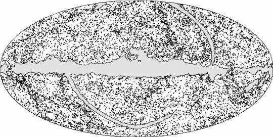
Figure 1: PSCz catalogue source distribution and related mask in galactic coordinates.

2.2 The Selection Function

No available galaxy catalogue is complete in volume and therefore completeness estimates derived from the selection effects in flux are needed. More in detail, the relevant quantity to be derived is the fraction of galaxies actually observed at the various redshifts, a quantity also known as the redshift selection function $\phi(z)$ [32]. A convenient way to express $\phi(z)$ is in terms of the galaxy luminosity function (i.e. the distribution of galaxy luminosities) $\Phi(L)$ as

$$\phi(z)=\frac{\int_{L_{\mathrm{min}}(z)}^{\infty}{\rm d}\,L\ \Phi(L)}{\int_{0}^{\infty}{\rm d}\,L\ \Phi(L)}.$$ (1)

Here $L_{\mathrm{min}}(z)$ is the minimum luminosity detected by the survey in function of redshift. By definition, for a flux-limited survey of limiting flux $f_{\rm lim}$, $L_{\mathrm{min}}(z)$ is given in terms of the luminosity distance $d_{L}(z)$ as

$$L_{\mathrm{min}}(z)=4\pi{d_{L}^{2}(z)}f_{\mathrm{lim}}.$$ (2)

The luminosity distance depends on the cosmology assumed, though for small redshifts ($z\;^{<}\!\!\!\!_{\sim}\;0.1$) it can be approximated by $d_{L}(z)\simeq z/H_{0}$.

Generally $\phi(z)$ is inferred from the catalogue data itself in a self-consistent way, using the observational galaxy luminosity distribution to estimate $\Phi(L)$ [27, 33, 34]. The quantity $n(z)/\phi(z)$ represents the experimental distribution corrected for the selection effects, which must be used in the computations. A detailed discussion of this issue can be found in Ref. [35]. Furthermore, we wish to stress that up to $z\sim 0.1$ evolution effects are negligible and the local universe galaxy luminosity function can be safely used. In the case of deeper surveys like SDSS, cosmological effects cannot be neglected and our approach can still be employed even though a series of corrections, like evolutionary effects or scale-dependent luminosity, must be taken into account [36]. These corrections are needed since luminous galaxies, which dominate the sample at large scales, cluster more than faint ones [37]. In the case of the PSCz catalogue the selection function is given as [27]

$$\phi(r)=\phi_{*}{\left({\frac{r}{r_{*}}}\right)}^{1-\alpha}{\left[{1+{\left(\frac{r}{r_{*}}\right)}^{\gamma}}\right]}^{-\left(\beta\over\gamma\right)},$$ (3)

with the parameters $\phi_{*}=0.0077,\>\alpha=1.82,\>r_{*}=86.4,\>\gamma=1.56,\>\beta=4.43$ that respectively describe the normalization, the nearby slope, the break distance in $\,h^{-1}{\rm Mpc}$, its sharpness and the additional slope beyond the break (see also Fig. 2).

Figure 2: Experimental redshift distribution of the PSCz catalogue galaxies and prediction for an homogeneous universe from the selection function $\phi(z)$ (from [27]); both are normalized in order to represent the number of sources per unit of redshift per steradian.

It is clear, however, that even taking into account the selection function we cannot use the catalogue up to the highest redshifts ($z\simeq 0.3$), due to the rapid loss of statistics. At high $z$, in fact, the intrinsic statistical fluctuation due to the selection effect starts to dominate over the true matter fluctuations, producing artificial clusterings not corresponding to real structures (“shot noise” effect). This problem is generally treated constructing from the point sources catalogue a smoothed density field $\rho(\hat{\Omega},z)$ with a variable smoothing length that effectively increases with redshift, remaining always of size comparable to the mean distance on the sphere of the sources of the catalogue. We minimize this effect by being conservative in setting the maximum redshift at $z=0.06$ (corresponding to $180\,h^{-1}{\rm Mpc}$) where we have still good statistics while keeping the shot noise effect under control. With this threshold we are left with $\sim 11,500$ sources of the catalogue. Furthermore, for the purposes of present analysis, the weight of the sources rapidly decreases with redshift due to the energy losses induced by the GZK effect. In the energy range $E\geq\,$5${\times}10^{19}\,$eV, the contribution from sources beyond $z\simeq 0.06$ is sub-dominant, thus allowing to assume for the objects beyond $z=0.06$ an effective isotropic source contribution.

3 The Formalism

In the following we describe in some detail the steps involved in our formalism. In Sec. 3.1 we summarize our treatment for energy losses, in Sec. 3.2 the way the “effective” UHECR map is constructed, and in Sec. 3.3 the statistical analysis we perform.

3.1 UHECRs Propagation

The first goal of our analysis is to obtain the underlying probability distribution $f_{\rm LSS}(\hat{\Omega},E)$ to have a UHECR with energy higher than $E$ from the direction $\hat{\Omega}$. For simplicity here and throughout the paper we shall assume that each source of our catalogue has the same probability to emit a UHECR, according to some spectrum at the source $g(E_{i})$. In principle, one would expect some correlation of this probability with one or more properties of the source, like its star formation rate, radio-emission, size, etc. The authors of Ref. [26] tested for a correlation $L_{\rm UHECR}\propto L_{\rm FIR}^{\kappa}$, $L_{\rm UHECR}$ being the luminosity in UHECRs and $L_{\rm FIR}$ the one in far-infrared region probed in IRAS catalogue. The results of their analysis do not change appreciably as long as $0\;^{<}\!\!\!\!_{\sim}\;\kappa\;^{<}\!\!\!\!_{\sim}\;1$. We can then expect that our limit of $\kappa=0$ might well work for a broader range in parameter space, but this is not of much concern here, since we do not stick to specific models for UHECR sources. The method we discuss can be however easily generalized to such a case, and eventually also to a multi-parametric modelling of the correlation.

In an ideal world where a volume-complete catalogue were available and no energy losses for UHECRs were present, each source should then be simply weighted by the geometrical flux suppression $\propto d_{L}^{-2}$. The selection function already implies the change of the weight into $\phi^{-1}d_{L}^{-2}$. Moreover, while propagating to us, high-energy protons lose energy as a result of the cosmological redshift and of the production of $e^{\pm}$ pairs and pions (the dominant process) caused by interactions with CMB. For simplicity, we shall work in the continuous loss approximation [38]. Then, a proton of energy $E_{i}$ at the source at $z=z_{i}$ will be degraded at the Earth ($z=0$) to an energy $E_{f}$ given by the energy-loss equation

$$\frac{1}{E}\frac{dE}{dz}=-\frac{dt}{dz}{\times}(\beta_{\rm rsh}+\beta_{\pi}+\beta_{e^{\pm}}).$$ (4)

Eq.(4) has to be integrated from $z_{i}$, where the initial Cauchy condition $E(z=z_{i})=E_{i}$ is imposed, to $z=0$. The different terms in Eq. (4) are explicitly shown below

$$-\frac{dt}{dz} = [(1+z)H_{0}\sqrt{(1+z)^{3}\Omega_{M}+\Omega_{\Lambda}}]^{-1},$$ (5)

$$\beta_{\rm rsh}(z) = H_{0}\sqrt{(1+z)^{3}\Omega_{M}+\Omega_{\Lambda}},$$ (6)

$$\beta_{\pi}(z,E) \simeq C_{\pi}(1+z)^{3},\>\>E\geq E_{\rm match}$$ (8)

$$A_{\pi}(1+z)^{3}e^{-\frac{B_{\pi}}{E(1+z)}},\>\>E\leq E_{\rm match}$$

$$\beta_{e^{\pm}}(z,E) \simeq \frac{\alpha^{3}Z^{2}}{4\pi^{2}}\frac{m_{e}^{2}m_{p}^{2}}{E^{3}}\int_{2}^{\infty}{\rm d}\xi\frac{\varphi(\xi)}{\exp[\frac{m_{e}m_{p}\xi}{2ET_{0}(1+z)}]-1},$$ (9)

where we assume for the Hubble constant $H_{0}=71_{-3}^{+4}$ km/s/Mpc, and $\Omega_{M}\simeq 0.27$ and $\Omega_{\Lambda}\simeq 0.73$ are the matter and cosmological constant densities in terms of the critical one [39]. In the previous formulae, $m_{e}$ and $m_{p}$ are respectively the electron and proton masses, $T_{0}$ is the CMB temperature, and $\alpha$ the fine-structure constant. Since we are probing the relatively near universe, the results will not depend much from the cosmological model adopted, but mainly on the value assumed for $H_{0}$. More quantitatively, the r.h.s of Eq. (4) changes linearly with $H_{0}^{-1}$ (apart for the negligible term $\beta_{\rm rsh}$), while even an extreme change from the model ($\Omega_{M}=0.27$; $\Omega_{\Lambda}=0.73$) to ($\Omega_{M}=1$; $\Omega_{\Lambda}=0.0$) (the latter ruled out by present data) would only modify the energy loss term by 6% at $z\simeq 0.06$, the highest redshift we consider.

The parameterization for $\beta_{\pi}$ as well as the values $\{A_{\pi},B_{\pi},C_{\pi}\}=\{3.66{\times}10^{-8}{\rm yr}^{-1},2.87{\times}10^{20}\,{\rm eV},2.42{\times}10^{-8}{\rm yr}^{-1}\}$ are taken from [40], and $E_{\rm match}(z)=6.86\,e^{-0.807\,z}{\times}10^{20}\,$eV is used to ensure continuity to $\beta_{\pi}(z,E)$. An useful parameterization of the auxiliary function $\varphi(\xi)$ can be found in [41], which we follow for the treatment of the pair production energy loss. In practice, we have evolved cosmic rays over a logarithmic grid in $E_{i}$ from $10^{19}$ to $10^{23}$ eV, and in $z$ from 0.001 to 0.3. The values at a specific source site has been obtained by a smooth interpolation.

Note that in our calculation i) the propagation is performed to attribute an “energy-loss weight” to each $z$ in order to derive a realistic probability distribution $f_{\rm LSS}(\hat{\Omega},E)$; ii) we are going to “smooth” the results over regions of several degrees in the sky (see below), thus performing a sort of weighted average over redshifts as well. Since this smoothing effect is by far dominant over the single source stochastic fluctuation induced by pion production, the average effect accounted for by using a continuous energy-loss approach is a suitable approximation.

In summary, the propagation effects provide us a “final energy function” $E_{f}(E_{i},z)$ giving the energy at Earth for a particle injected with energy $E_{i}$ at a redshift $z$. Note that, being the energy-loss process obviously monotone, the inverse function $E_{i}(E_{f},z)$ is also available.

3.2 Map Making

Given an arbitrary injection spectrum $g(E_{i})$, the observed events at the Earth would distribute, apart for a normalization factor, according to the spectrum $g(E_{i}(E_{f},z))dE_{i}/dE_{f}$. In particular we will consider in the following a typical power-law $g(E_{i})\propto E_{i}^{-s}$, but this assumption may be easily generalized. Summing up on all the sources in the catalogue one obtains the expected differential flux map on Earth

$$F(\hat{\Omega},E_{f})\propto\sum_{k}\frac{1}{\phi(z_{k})}\frac{\delta(\hat{\Omega}-\hat{\Omega}_{k})}{4\pi d^{2}_{L}(z_{k})}E_{i}^{-s}(E_{f},z_{k})\frac{dE_{i}}{dE_{f}}(E_{f},z_{k}),$$ (10)

where the selection function and distance flux suppression factors have been taken into account. However, given the low statistics of events available at this high energies, a more useful quantity to employ is the integrated flux above some energy threshold $E_{\rm cut}$, that can be more easily compared with the integrated UHECR flux above the cut $E_{\rm cut}$. Integrating the previous expression we have

$$f_{\rm LSS}(\hat{\Omega},E_{\rm cut}) \propto \sum_{k}\frac{1}{\phi(z_{k})}\frac{\delta(\hat{\Omega}-\hat{\Omega}_{k})}{4\pi d^{2}_{L}(z_{k})}\int_{E_{i}(E_{\rm cut},z_{k})}^{\infty}\!\!\!\!\!\!E^{-s}{\rm d}E$$ (11)

$$= \sum_{k}f_{\rm LSS}(k)\ \delta(\hat{\Omega}-\hat{\Omega}_{k}),$$

that can be effectively seen as if at every source $k$ of the catalogue it is assigned a weight $f_{\rm LSS}(k)$ that takes into account geometrical effects ($d_{L}^{-2}$), selection effects ($\phi^{-1}$), and physics of energy losses through the integral in d$E$. In this “GZK integral” the upper limit of integration is taken to be infinite, though the result is practically independent from the upper cut used provided it is much larger than 10²⁰ eV.

It is interesting to compare the similar result expected for an uniform source distribution with constant density; in this case we have (in the limit $z\ll 1$)

$$f_{\rm LSS}(\hat{\Omega},E_{\rm cut})\propto\int{\rm d}z\frac{\left[E_{i}(E_{\rm cut},z)\right]^{-s+1}}{s-1}\equiv\int{\rm d}z\,p(z,E_{\rm cut},s),$$ (12)

where the integral in d$E$ has been explicitly performed and the flux suppression weight is cancelled by the geometrical volume factor. The integrand $p(z,E_{\rm cut},s)$ containing the details of the energy losses also provides an effective cut at high $z$. The integrand —when normalized to have unit area— can be interpreted as the distribution of the injection distances of CR observed at the Earth. It also suggests the definition of the so-called “GZK sphere” as the sphere from which originates most (say 99%) of the observed CR flux on Earth above an energy threshold $E_{\rm cut}$. In Fig. 3 we plot the distribution $p$ for different values of $E_{\rm cut}$ and $s$. We see that around a particular threshold $z_{\rm GZK}$ the distribution falls to zero: the dependence of $z_{\rm GZK}$ on $E_{\rm cut}$ is quite critical as expected, while there is also a softer dependence on $s$. This suggests naturally the choice $E_{\rm cut}=5{\times}10^{19}\,$eV for the chosen value $z_{\rm GZK}\simeq 0.06$; at the same time, the energy cut chosen is not too restrictive, ensuring indeed that a significant statistics might be achieved in a few years. For this $E_{\rm cut}$ the isotropic contribution to the flux is sub-dominant; however we can take it exactly into account and the weight of the isotropic part is given by

$$w_{\rm iso}\propto\int_{z_{\rm GZK}}^{\infty}{\rm d}z\,p(z,E_{\rm cut}).$$ (13)

Finally, to represent graphically the result, the spike-like map (11) is effectively smoothed through a gaussian filter as

$$f_{\rm LSS}(\hat{\Omega},E_{\rm cut})\propto\sum_{k}f_{\rm LSS}(k)\exp\left(-\frac{d_{s}^{2}[\hat{\Omega},\hat{\Omega}_{k}]}{2\sigma^{2}}\right)+\frac{w_{\rm iso}}{4\pi}2\pi\sigma^{2}\mu(\hat{\Omega}).$$ (14)

In the previous equation, $\sigma$ is the width of the gaussian filter, $d_{s}$ is the spherical distance between the coordinates $\hat{\Omega}$ and $\hat{\Omega}_{k}$, and $\mu(\hat{\Omega})$ is the catalogue mask (see Section 2.1) such that $\mu(\hat{\Omega})=0$ if $\hat{\Omega}$ belongs to the mask region and $\mu(\hat{\Omega})=1$ otherwise.

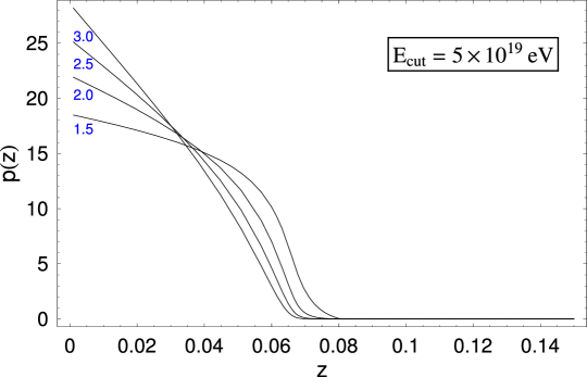
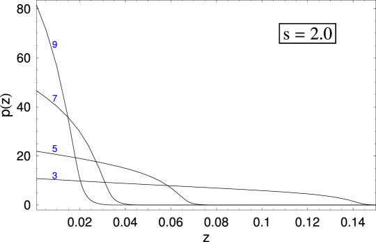
Figure 3: Distribution of the injection distances of CR observed at the Earth for fixed $E_{\rm cut}=5{\times}10^{19}$ eV (top) and $s=1.5,2.0,2.5,3.0$ and for fixed spectral index $s=2.0$ (bottom) and varying $E_{\rm cut}=3,5,7,9{\times}10^{19}$ eV. The area subtended by $p(z)$ has been normalized to unity.

3.3 Statistical Analysis

Given the extremely poor UHECR statistics, we limit ourselves to address the basic issue of determining the minimum number of events needed to significatively reject “the null hypothesis”. To this purpose, it is well known that a $\chi^{2}$-test is an extremely good estimator. Notice that a $\chi^{2}$-test needs a binning of the events, but differently from the K-S test performed in [26] or the Smirnov-Cramer-von Mises test of [25], it has no ambiguity due to the 2-dimensional nature of the problem, and indeed a similar approach was used in [23]. A criterion guiding in the choice of the bin size is the following: with $N$ UHECRs events available and $M$ bins, one would expect ${\cal O}(N/M)$ events per bin; to allow a reliable application of the $\chi^{2}$-test, one has to impose $N/M\geq 10$. Each cell should then cover at least a solid angle of $\Delta_{M}\sim 10{\times}\Delta_{\rm tot}/N$, $\Delta_{\rm tot}$ being the solid angle accessible to the experiment. For $\Delta_{\rm tot}\sim 2\pi$ (50% of full sky coverage), one estimates a square window of side $454^{\circ}/\sqrt{N}$, i.e. $45^{\circ}$ for 100 events, $14^{\circ}$ for 1000 events. Since the former number is of the order of present world statistics, and the latter is the achievement expected by Auger in several years of operations, a binning in windows of size $15^{\circ}$ represents quite a reasonable choice for our forecast. This choice is also suggested by the typical size of the observable structures, a point we will comment further at the end of this Section. Notice that the GMF, that induces at these energies typical deflections of about $4^{\circ}$ [43], can be safely neglected for this kind of analysis. The same remark holds for the angular resolution of the experiment.

Obviously, for a specific experimental set-up one must include the proper exposure $\omega_{\rm exp}$, to convolve with the previously found $f_{\rm LSS}$. The function $\omega_{\rm exp}$ depends on the declination $\delta$, right ascension RA, and, in general, also on the energy. For observations having uniform coverage in RA, like AGASA or Auger ground based arrays, one can easily parameterize the relative exposure as [42]

$$\omega_{\rm exp}(\delta)\propto\cos\theta_{0}\sin\alpha_{m}\cos\delta+\alpha_{m}\sin\theta_{0}\sin\delta,$$ (15)

where $\theta_{0}$ is the latitude of the experiment ($\theta_{0}\approx-35^{\circ}$ for Auger South), $\alpha_{m}$ is given by

$$\alpha_{m}=\left\{\begin{array}[]{ll}0\,,&{\rm if}\,\,\,\xi>1\\ \pi\,,&{\rm if}\,\,\,\xi<-1\\ \cos^{-1}\xi\,,&{\rm otherwise}\end{array}\right.$$ (16)

and

$$\xi\equiv\frac{\cos\theta_{\rm max}-\sin\theta_{0}\,\,\sin\delta}{\cos\theta_{0}\,\,\,\cos\delta}\,\,,$$ (17)

$\theta_{\rm max}$ being the maximal zenith angle cut applied (we assume $\theta_{\rm max}=60^{\circ}$ for Auger). Contour plots for the Auger exposure function in galactic coordinates are shown in Fig. 4.

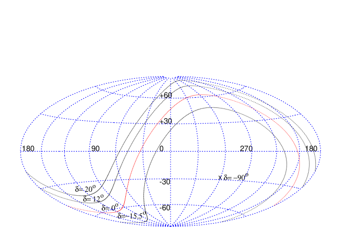
Figure 4: Galactic coordinate reference frame and contours enclosing 68%, 95% and 99% of the Auger exposure function, with the corresponding declinations. The celestial equator ($\delta=0^{\circ}$) and south pole ($\delta=-90^{\circ}$) are also shown.

For a given experiment and catalogue, the null hypothesis we want to test is that the events observed are sampled —apart from a trivial geometrical factor— according to the distribution $f_{\rm LSS}\,\omega_{\rm exp}\,\mu$. Since we are performing a forecast analysis, we will consider test realizations of $N$ events sampled according to a random distribution on the (accessible) sphere, i.e. according to $\omega_{\rm exp}\,\mu$, and determine the confidence level (C.L.) with which the hypothesis is rejected as a function of $N$. For each realization of $N$ events we calculate the two functions

$${\cal X}_{\rm iso}^{2}(N)=\frac{1}{M-1}\sum_{i=1}^{M}\frac{(o_{i}-\epsilon_{i}[f_{\rm iso}])^{2}}{\epsilon_{i}[f_{\rm iso}]},$$ (18)

$${\cal X}_{\rm LSS}^{2}(N)=\frac{1}{M-1}\sum_{i=1}^{M}\frac{(o_{i}-\epsilon_{i}[f_{\rm LSS}])^{2}}{\epsilon_{i}[f_{\rm LSS}]},$$ (19)

where $o_{i}$ is the number of “random” counts in the $i$-th bin $\Omega_{i}$, and $\epsilon_{i}[f_{\rm LSS}]$ and $\epsilon_{i}[f_{\rm iso}]$ are the theoretically expected number of events in $\Omega_{i}$ respectively for the LSS and isotropic distribution. In formulae (see Eq. (11)),

$$\epsilon_{i}[f_{\rm LSS}] = N\alpha\frac{\sum_{j\in\Omega_{i}}f_{\rm LSS}(j)\omega_{\rm exp}(\delta_{j})\mu(j)+w_{\rm iso}/4\pi\,S[\Omega_{i}]}{\sum_{j}f_{\rm LSS}(j)\omega_{\rm exp}(\delta_{j})\mu(j)+w_{\rm iso}/4\pi\,S_{\omega}},$$ (20)

$$\epsilon_{i}[f_{\rm iso}] = N\alpha\frac{S[\Omega_{i}]}{S_{\omega}},$$ (21)

where $S[\Omega_{i}]=\int_{\Omega_{i}}\!\!d\Omega\,\omega_{\rm exp}\mu$ is the spherical surface (exposure- and mask-corrected) subtended by the angular bin $\Omega_{i}$, and similarly $S_{\omega}=\int_{4\pi}\!\!d\Omega\,\omega_{exp}\mu$. The mock data set is then sampled ${\cal N}$ times in order to establish empirically the distributions of ${\cal X}_{\rm LSS}^{2}$ and ${\cal X}_{\rm iso}^{2}$, and the resulting distribution is studied as function of $N$ (plus eventually $s,E_{\rm cut}$, etc.). The parameter

$$\alpha\equiv\frac{\int d\Omega\ \omega_{exp}(\delta)\mu(\Omega)}{\int d\Omega\ \omega_{exp}(\delta)}$$ (22)

is a mask-correction factor that takes into account the number of points belonging to the mask region and excluded from the counts $o_{i}$. Note that the random distribution is generated with $N$ events in all the sky view of the experiment, but, effectively, only the region outside the mask is included in the statistical analysis leaving us with effective $N\alpha$ events to study. This is a limiting factor due to quality of the catalogue: With a better sky coverage the statistics is improved and the number of events required to asses the model can be reduced.

As our last point, we return to the problem of choice of the bin size. To assess its importance we studied the dependence of the results on this parameter. For a cell side larger than about $\sim 25^{\circ}$ the analysis loses much of its power, and a very high $N$ is required to distinguish the models and obtain meaningful conclusions. This is somewhat expected looking at the map results that we obtain, where typical structures have dimensions of the order $15^{\circ}-20^{\circ}$. A greater cell size results effectively in a too large smoothing and a consequent lost of information. On the other hand, a cell size below $4^{\circ}-6^{\circ}$ makes the use of a $\chi^{2}$ analysis not very reliable, because of the low number of events in each bin expected for realistic exposure times. In the quite large interval $\sim 6^{\circ}-20^{\circ}$ for the choice of the cell size, however, the result is almost independent of the bin size, that makes us confident on the reliability of our conclusions.

4 Results

In Fig. 5 we plot the smoothed maps in galactic coordinates of the expected integrated flux of UHECRs above the energy threshold $E_{\rm cut}=3,5,7,9{\times}10^{19}\,$eV and for slope parameter $s=2.0$; the isotropic part has been taken into account and the ratio of the isotropic to anisotropic part $w_{\rm iso}/\sum_{k}f_{\rm LSS}(k)$ is respectively $83\%,3.6\%,\ll 1\%,\ll 1\%$.

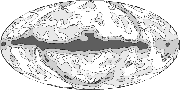
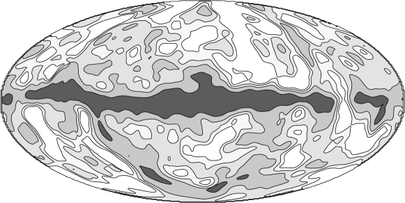
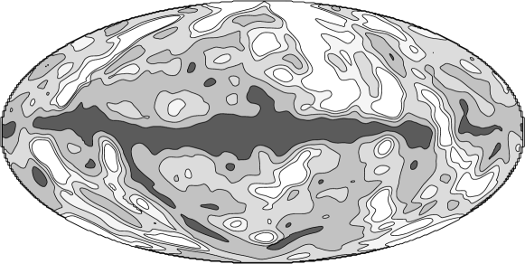
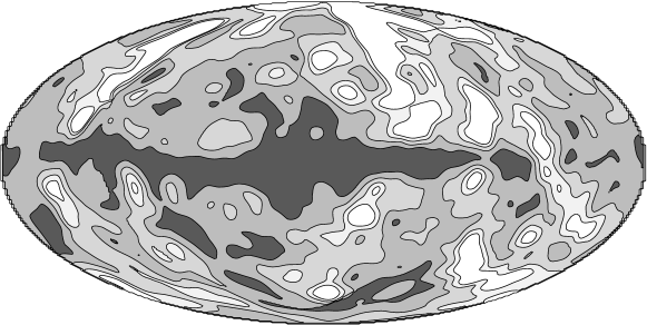
Figure 5: Equal area Hammer-Aitoff projections of the smoothed UHECRs arrival directions distribution (Eq. (14)) in galactic coordinates obtained for fixed $s=2.0$ and, from the upper to the lower panel, for $E_{\rm cut}=3,5,7,9{\times}10^{19}$ eV. The smoothing angle is $\sigma=3^{\circ}$. The contours enclose 95%, 68%, 38%, 20% of the corresponding distribution.

Only for $E_{\rm cut}=3{\times}10^{19}\,$eV the isotropic background constitutes then a relevant fraction, since the GZK suppression of far sources is not yet present. For the case of interest $E_{\rm cut}=5{\times}10^{19}\,$eV the contribution of $w_{\rm iso}$ is almost negligible, while it practically disappears for $E_{\rm cut}\raise 1.29167pt\hbox{$\;>$\kern-7.5pt\raise-4.73611pt\hbox{$\sim\;$}}7{\times}10^{19}\,$eV. Varying the slope for $s=1.5,2.0,2.5,3.0$ while keeping $E_{\rm cut}=5{\times}10^{19}\,$eV fixed produces respectively the relative weights $8.0\%,3.6\%,1.8\%,0.9\%$, so that only for very hard spectra $w_{\rm iso}$ would play a non-negligible role (see also Fig. 3).

Due to the GZK-effect, as it was expected, the nearest structures are also the most prominent features in the maps. The most relevant structure present in every slide is the Local Supercluster. It extends along $l\simeq 140^{\circ}$ and $l\simeq 300^{\circ}$ and includes the Virgo cluster at $l=284^{\circ},b=+75^{\circ}$ and the Ursa Major cloud at $l=145^{\circ},b=+65^{\circ}$, both located at $z\simeq 0.01$. The lack of structures at latitudes from $l\simeq 0^{\circ}$ to $l\simeq 120^{\circ}$ corresponds to the Local Void. At higher redshifts the main contributions come from the Perseus-Pisces supercluster ($l=160^{\circ},b=-20^{\circ}$) and the Pavo-Indus supercluster ($l=340^{\circ},b=-40^{\circ}$), both at $z\sim 0.02$, and the very massive Shapley Concentration ($l=250^{\circ},b=+20^{\circ}$) at $z\sim 0.05$. For a more detailed list of features in the map, see the key in Fig. 6.

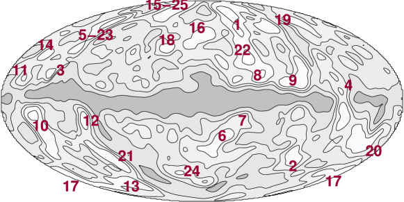
Figure 6: Detailed key of the structures visible in the UHECR maps; arbitrary contour levels. Labels correspond to: (1) Southern extension of Virgo and Local Supercluster; (2)Fornax-Eridani Cluster; (3) Cassiopea Cluster; (4) Puppis Cluster; (5) Ursa Major Cloud; (6-7) Pavo-Indus and ”Great Attractor” region; (8) Centaurus Super-Cluster; (9) Hydra Super-Cluster; (10) Perseus Super-Cluster; (11) Abell 569; (12) Pegasus Cluster; (13-17) Pisces Cluster; (14) Abell 634; (15) Coma Cluster; (16-18) Hercules Supercluster; (19) Leo Supercluster; (20) Columba Cluster; (21) Cetus Cluster; (22) Shapley Concentration; (23) Ursa Major Supercluster; (24) Sculptor Supercluster; (25) Bootes Supercluster.

The $E_{\rm cut}$-dependence is clearly evident in the maps: as expected, increasing $E_{\rm cut}$ results in a map that closely reflects the very local universe (up to $z\sim 0.03-0.04$) and its large anisotropy; conversely, for $E_{\rm cut}\simeq 3,4{\times}10^{19}\,$eV, the resulting flux is quite isotropic and the structures emerge as fluctuations from a background, since the GZK suppression is not yet effective. This can be seen also comparing the near structures with the most distant ones in the catalogue: while the Local Supercluster is well visible in all slides, the signal from the Perseus-Pisces super-cluster and the Shapley concentration is of comparable intensity only in the two top panels, while becoming highly attenuated for $E_{\rm cut}=7{\times}10^{19}\,$eV, and almost vanishing for $E_{\rm cut}=9{\times}10^{19}\,$eV. A similar trend is observed for increasing $s$ at fixed $E_{\rm cut}$, though the dependence is almost one order of magnitude weaker. Looking at the contour levels in the maps we can have a precise idea of the absolute intensity of the “fluctuations” induced by the LSS; in particular, for the case of interest of $E_{\rm cut}=5{\times}10^{19}\,$eV the structures emerge only at the level of 20%-30% of the total flux, the 68% of the flux actually enclosing almost all the sky. For $E_{\rm cut}=7,9{\times}10^{19}\,$eV, on the contrary, the local structures are significantly more pronounced, but in this case we have to face with the low statistics available at this energies. Then in a low-statistics regime it’s not an easy task to disentangle the LSS and the isotropic distributions.

$N\setminus s$	1.5	2.0	2.5	3.0
50	(42:6)	(47:8)	(52:10)	(52:10)
100	(55:9)	(60:12)	(66:14)	(69:16)
200	(72:27)	(78:33)	(84:40)	(86:43)
400	(92:61)	(95:72)	(97:80)	(98:83)
600	(98:85)	(99:91)	(100:96)	(100:97)
800	(100:95)	(100:98)	(100:99)	(100:100)
1000	(100:98)	(100:100)	(100:100)	(100:100)

Table 1: The probability (in %) to reject the isotropic hypothesis at (90%:99%) C.L. when UHECRs follow the LSS distribution, as a function of the injection spectral index and of the observed number of events, fixing $E_{\rm cut}=5{\times}10^{19}\,$eV.

The structures which are more likely to be detected by Auger (see also Fig. 4) are the Shapley concentration, the Southern extension of the Virgo cluster, the Local Supercluster and the Pavo-Indus super-cluster. Other structures, such as the Perseus-Pisces supercluster and the full Virgo cluster are visible only from the Northern hemisphere and are therefore within the reach of experiments like Telescope Array [44], or the planned North extension of the Pierre Auger Observatory. Moreover, the sky region obscured by the heavy extinction in the direction of the Galactic Plane reflects a lack of information about features possibly “hidden” there. Unfortunately, this region falls just in the middle of the Auger field of view, thus reducing —for a given statistics $N$— the significance of the check of the null hypothesis. Numerically, this translates into a smaller value of the factor $\alpha$ of Eq. (22) with respect to an hypothetical “twin” Northern Auger experiment.

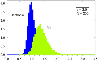
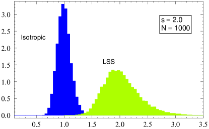
Figure 7: The probability distributions of the estimators ${\cal X}_{\rm iso}^{2}$ and ${\cal X}_{\rm LSS}^{2}$ for the cases $s=2.0,3.0$ and for $N=200,1000$ events, fixing $E_{\rm cut}=5{\times}10^{19}\,$eV. The distribution are the results of 10000 monte-carlo simulation like described in the text.

A quantitative statistical analysis confirms previous qualitative considerations. In Table 1 we report the probability to reject the isotropic hypothesis at 90% and 99% C.L. when UHECRs follow the LSS distribution, as a function of the injection spectral index and of the observed number of events, fixing $E_{\rm cut}=5{\times}10^{19}\,$eV. In Figure 7 we show the distributions of the functions ${\cal X}_{\rm iso}^{2}$ and ${\cal X}_{\rm LSS}^{2}$ introduced in the previous section for $s=2.0,3.0$ and $N=200,1000$, for the same cut $E_{\rm cut}=5{\times}10^{19}\,$eV. It is clear that a few hundreds events are hardly enough to reliably distinguish the two models, while $N=\,$800–1000 should be more than enough to reject the hypothesis at 2-3$\,\sigma$, independently of the injection spectrum. Steeper spectra however slightly reduce the number of events needed for a given C.L. discrimination. It is also interesting to note that, using different techniques and unconstrained LSS simulations, it was found that a comparable statistics is needed to probe a magnetized local universe [17]. It is worthwhile stressing that our conclusions should be looked as conservative, since only proton primaries have been assumed, and constant source properties. Variations in individual source power and a mixed composition could increase the “cosmic variance” and make more difficult to distinguish among models for the source distribution [17].

With respect to previous literature on the subject, our analysis is the closest to the one of Ref. [23]. Apart for technical details, the greatest differences with respect to this work arise because of the improved determination of crucial parameters undergone in the last decade. Just to mention a few, the Hubble constant used in [23] was 100 km s^-1 Mpc^-1, against the presently determined value of $71_{-3}^{+4}$ km s^-1 Mpc^-1: this changes by a 30% the value of the quantity $z_{\rm GZK}$ (see Sec. 3.2). Moreover, the catalogue [45] that was used in [23] contains about 1/3 of the objects we are considering, has looser selection criteria and larger contaminations [27]. Finally, the specific location of the Southern Auger observatory was not taken into account. All together, when considering these factors, we find quite good agreement with their results.

Some discrepancy arises instead with the results of [26], whose maps appear to be dominated by statistical fluctuations, which mostly wash away physical structures. This has probably to be ascribed to two effects, the energy cut $E_{\rm cut}=4{\times}10^{19}\,$eV and the inclusion of high redshift object (up to $z\sim 0.3$) of the catalogue [27] in their analysis. Their choice of $E_{\rm cut}=4{\times}10^{19}\,$eV implies indeed $z_{\rm GZK}\simeq 0.1$, i.e. a cutoff in a redshift range where shot noise distortions are no longer negligible. The same remarks hold for Ref. [25], which also suffers of other missing corrections [26]. Also, in both cases, the emphasis is mainly in the analysis of the already existing AGASA data than in a forecast study. Our results however clearly show that AGASA statistics —only 32 data at $E\geq 5{\times}10^{19}\,$eV in the published data set [46], some of which falling inside the mask— is too limited to draw any firm conclusion on the hypothesis considered.

5 Summary and conclusion

In this work we have summarized the technical steps needed to properly evaluate the expected anisotropy in the UHECR sky starting from a given catalogue of the local universe, taking into account the selection function, the blind regions, and the energy-loss effects. By applying this method to the catalogue [27], we have established the minimum statistics needed to significatively reject the null hypothesis, in particular providing a forecast for the Auger experiment. We showed with a $\chi^{2}$ approach that several hundreds data are required to start testing the model at Auger South. The most prominent structures eventually “visible” for this experiment were also identified.

Differently from other statistical tools based e.g. on auto-correlation analysis, the approach sketched above requires an Ansatz on the source candidates. The distribution of the luminous baryonic matter considered here can be thought as a quite generic expectation deserving interest of its own, but it is also expected to correlate with many sources proposed in the literature. In any case, if many astrophysical sources are involved in UHECR production, it is likely that they should better correlate with the local baryonic matter distribution than with an isotropic background.

As already stated, this work has to be intended as mainly methodological. Until now, the lack of UHECR statistics and the inadequacy of the astronomical catalogues has seriously limited the usefulness of such a kind of analysis. However, progresses are expected in both directions in forthcoming years. From the point of view of UHECR observatories, the Southern site of Auger is almost completed, and already taking data. Working from January 2004 to June 2005, Auger has reached a cumulative exposure of 1750 km² sr yr, observing 10 events over 10${}^{19.7}\,$eV=5${\times}10^{19}\,$eV (see the URL: www.auger.org/icrc2005/spectrum.html), Notice that statistical and systematic errors are still quite large, and a down-shift in the $\log_{10}E$ scale of 0.1 would for example change the previous figure to 17 events. Once completed, the total area covered will be of 3000 km², thus improving by one order of magnitude present statistics in a couple of years [47]. The idea to build a Northern Auger site strongly depends on the possibility to perform UHECR astronomy, for which full sky coverage is of primary importance. In any case, the Japanese-American Telescope Array in the desert of Utah is expected to become operational by 2007 [48]. It should offer almost an order of magnitude larger aperture per year than AGASA in the Northern sky, with a better control over the systematics thanks to a hybrid technique similar to the one employed in Auger.

The other big step is expected in astronomical catalogues. The 2MASS survey [28] has resolved more than 1.5 million galaxies in the near-infrared, and has been explicitly designed to provide an accurate photometric and astrometric knowledge of the nearby Universe. The observation in the near IR is particularly sensitive to the stellar component, and as a consequence to the luminous baryons. Though the redshifts of the sources have to be obtained via photometric methods, the larger error on the distance estimates (about 20% from the 3-band 2MASS photometry [29]) is more than compensated by the larger statistics. An analysis of this catalogue for UHECR purposes is in progress. Independently of large sky coverage, deep surveys like SDSS [31] undoubtedly have an important role in mapping the local universe as well. For example, the information encoded in such catalogues can be used to validate methods —like the neural networks [49, 50, 51]— used to obtain photometric redshifts. An even better situation is expected from future projects like SDSS II (see the URL: www.sdss.org). Finally, a by-product of these surveys is the discovery and characterization of active galactic nuclei [52, 53], which in turn could have interesting applications in the search for the sources of UHECRs.

References

References

- [1] E. Roulet, “Astroparticle theory: Some new insights into high energy cosmic rays,” Int. J. Mod. Phys. A 19, 1133 (2004) [astro-ph/0310367].
- [2] K. Greisen, “End To The Cosmic Ray Spectrum?,” Phys. Rev. Lett. 16, 748 (1966).
- [3] G. T. Zatsepin and V. A. Kuzmin, “Upper Limit Of The Spectrum Of Cosmic Rays,” JETP Lett. 4, 78 (1966) [Pisma Zh. Eksp. Teor. Fiz. 4, 114 (1966)].
- [4] Linsley, “Evidence for a Primary Cosmic-Ray Particle with Energy 10**20 eV”, Phys. Rev. Lett. 10, 146 (1963).
- [5] M. M. Winn et al.[SUGAR Collaboration], “The Cosmic Ray Energy Spectrum Above 10**17-Ev,” J. Phys. G 12, 653 (1986).
- [6] M. A. Lawrence, R. J. O. Reid and A. A. Watson [Haverah Park Collaboration], “The Cosmic ray energy spectrum above 4x10**17-eV as measured by the Haverah Park array,” J. Phys. G 17, 733 (1991).
- [7] M. Ave et al. [Haverah Park Collaboration], “New constraints from Haverah Park data on the photon and iron fluxes of UHE cosmic rays,” Phys. Rev. Lett. 85, 2244 (2000) [astro-ph/0007386].
- [8] D. J. Bird et al. [Fly’s Eye Collaboration], “Evidence for correlated changes in the spectrum and composition of cosmic rays at extremely high-energies,” Phys. Rev. Lett. 71, 3401 (1993).
- [9] D. J. Bird et al. [Fly’s Eye Collaboration], “The Cosmic ray energy spectrum observed by the Fly’s Eye,” Astrophys. J. 424, 491 (1994).
- [10] D. J. Bird et al. [Fly’s Eye Collaboration], “Detection of a cosmic ray with measured energy well beyond the expected spectral cutoff due to cosmic microwave radiation,” Astrophys. J. 441, 144 (1995).
- [11] N.N. Efimov et al. [Yakutsk Collaboration], “The Energy Spectrum and Anisotropy of primary cosmic rays at energy E(0)eV observed in Yakutsk”, in Proceedings of Astrophysical Aspects of the Most Energetic Cosmic Rays, (World Scientific, Singapore, 1991).
- [12] M. Takeda et al. [AGASA Collaboration], “Extension of the cosmic-ray energy spectrum beyond the predicted Greisen-Zatsepin-Kuzmin cutoff,” Phys. Rev. Lett. 81, 1163 (1998) [astro-ph/9807193].
- [13] R. U. Abbasi et al. [HiRes Collaboration], “Measurement of the flux of ultrahigh energy cosmic rays from monocular observations by the High Resolution Fly’s Eye experiment,” Phys. Rev. Lett. 92, 151101 (2004) [astro-ph/0208243].
- [14] T. Abu-Zayyad et al. [HiRes Collaboration], “Measurement of the spectrum of UHE cosmic rays by the FADC detector of the HiRes experiment,” Astropart. Phys. 23, 157 (2005) [astro-ph/0208301].
- [15] P. Sommers [Pierre Auger Collaboration], “First estimate of the primary cosmic ray energy spectrum above 3-EeV from the Pierre Auger observatory,” astro-ph/0507150, to appear in the Proceedings of the 29th ICRC, (2005) Pune (India).
- [16] K. Dolag, D. Grasso, V. Springel and I. Tkachev, “Mapping deflections of Ultra-High Energy Cosmic Rays in Constrained Simulations of Extragalactic Magnetic Fields,” JETP Lett. 79, 583 (2004) [Pisma Zh. Eksp. Teor. Fiz. 79, 719 (2004)] [astro-ph/0310902]; See also “Constrained simulations of the magnetic field in the local universe and the propagation of UHECRs,” JCAP 0501, 009 (2005) [astro-ph/0410419].
- [17] G. Sigl, F. Miniati and T. A. Ensslin, “Ultra-high energy cosmic ray probes of large scale structure and magnetic fields,” Phys. Rev. D 70, 043007 (2004) [astro-ph/0401084]. See also “Cosmic magnetic fields and their influence on ultra-high energy cosmic ray propagation,” Nucl. Phys. Proc. Suppl. 136, 224 (2004) [astro-ph/0409098].
- [18] T. Antoni et al. [The KASCADE Collaboration], “KASCADE measurements of energy spectra for elemental groups of cosmic rays: Results and open problems,” Astropart. Phys. 24, 1 (2005) [astro-ph/0505413].
- [19] M. Takeda et al. [AGASA collaboration], “Small-scale anisotropy of cosmic rays above 10**19-eV observed with the Akeno Giant Air Shower Array,” Astrophys. J. 522 225 (1999); [astro-ph/9902239]; See also M. Takeda et al., Proc. 27th ICRC, Hamburg, 2001.
- [20] R. U. Abbasi et al. [The HiRes Collaboration], “Search for point sources of ultra-high energy cosmic rays above 40-EeV using a maximum likelihood ratio test,” Astrophys. J. 623, 164 (2005) [astro-ph/0412617].
- [21] B. Revenu [Pierre Auger Collaboration], “First estimate of the primary cosmic ray energy spectrum above 3-EeV from the Pierre Auger observatory,” in Proceedings of the 29th ICRC, (2005) Pune India.
- [22] J. W. Cronin, Nucl. Phys. Proc. Suppl. 28B, 213 (1992); see also http://www.auger.org/.
- [23] E. Waxman, K. B. Fisher and T. Piran, “The signature of a correlation between 10**19-eV cosmic ray sources and large scale structure,” Astrophys. J. 483, 1 (1997) [astro-ph/9604005].
- [24] N. W. Evans, F. Ferrer and S. Sarkar, “The anisotropy of the ultra-high energy cosmic rays,” Astropart. Phys. 17, 319 (2002) [astro-ph/0103085].
- [25] A. Smialkowski, M. Giller and W. Michalak, “Luminous infrared galaxies as possible sources of the UHE cosmic rays,” J. Phys. G 28, 1359 (2002) [astro-ph/0203337].
- [26] S. Singh, C. P. Ma and J. Arons, “Gamma-ray bursts and magnetars as possible sources of ultra high energy cosmic rays: Correlation of cosmic ray event positions with IRAS galaxies,” Phys. Rev. D 69, 063003 (2004) [astro-ph/0308257].
- [27] W. Saunders et al., “The PSCz Catalogue,” Mon. Not. Roy. Astron. Soc. 317, 55 (2000) [astro-ph/0001117].
- [28] Jarrett, T.H., Chester, T., Cutri, R., Schneider, S., Skrutskie, M. & Huchra, J. 2000a, AJ, 119, 2498.
- [29] Jarrett, T.H., “Large Scale Structure in the Local Universe: The 2MASS Galaxy Catalog,” Publ. Astron. Soc. Aust. 21, 396 (2004) [astro-ph/0405069].
- [30] York, D. et al. 2000, AJ, 120, 1579
- [31] J. K. Adelman-McCarthy et al. [SDSS Collaboration], “The Fourth Data Release of the Sloan Digital Sky Survey,” astro-ph/0507711.
- [32] Peebles, P. J. E. 1980, “The Large-Scale Structure of the Universe” (Princeton, NJ: Princeton University Press)
- [33] Sandage, A., Tammann, G. A., & Yahil, A. 1979, “STY luminosity function fitting method”, Astrophys. J. 232, 352.
- [34] Efstathiou, G., Ellis, R. S., & Peterson, B. S. 1988, MNRAS, 232, 431
- [35] M. Blanton, P. Blasi and A. V. Olinto, “The GZK feature in our neighborhood of the universe,” Astropart. Phys. 15, 275 (2001) [astro-ph/0009466].
- [36] M. Tegmark et al. [SDSS Collaboration], “The 3D power spectrum of galaxies from the SDSS,” Astrophys. J. 606, 702 (2004) [astro-ph/0310725].
- [37] Davis, M., Meiksin, A., Strauss, M. A., da Costa, L. N., & Yahil, A. 1988, ApJ, 333, L9
- [38] Berezinskii,V. and Grigor’eva, S. I. 1988, A&A, 199, 1.
- [39] D. N. Spergel et al. [WMAP Collaboration], “First Year Wilkinson Microwave Anisotropy Probe (WMAP) observations: Determination of cosmological parameters,” Astrophys. J. Suppl. 148, 175 (2003) [astro-ph/0302209].
- [40] L. A. Anchordoqui, M. T. Dova, L. N. Epele and J. D. Swain, “Effect of the 3-K background radiation on ultrahigh energy cosmic rays,” Phys. Rev. D 55, 7356 (1997) [hep-ph/9704387].
- [41] M. J. Chodorowski,A. Zdziarski and M. Sikora, Astrophys. J. 400, 181 (1992).
- [42] P. Sommers, “Cosmic Ray Anisotropy Analysis with a Full-Sky Observatory,” Astropart. Phys. 14, 271 (2001) [astro-ph/0004016].
- [43] M. Kachelrieß P.D. Serpico, and M. Teshima, “The Galactic magnetic field as spectrograph for ultra-high energy cosmic rays,” astro-ph/0510444.
- [44] Y. Arai et al., “The Telescope Array experiment: An overview and physics aims,” Proceedings of 28th ICRC (2003), Tsukuba.
- [45] K.B. Fisher et al., Astrophys.J.Suppl. 100, 69 (1995)
- [46] N. Hayashida et al., “Updated AGASA event list above 4*10**19-eV,” Astron. J. 120, 2190 (2000) [astro-ph/0008102].
- [47] X. Bertou [Pierre Auger Collaboration], “Performance of the Pierre Auger Observatory surface array,” astro-ph/0508466, in the Proceedings of the 29th ICRC, (2005) Pune India.
- [48] K. Kasahara et al. [TA Collaboration], “The Current Status and Prospect of the Ta Experiment,” astro-ph/0511177.
- [49] R. Tagliaferri, G. Longo, S. Andreon, S. Capozziello, C. Donalek and G. Giordano, “Neural Networks and Photometric Redshifts,” astro-ph/0203445.
- [50] A. A. Collister and O. Lahav, “ANNz: estimating photometric redshifts using artificial neural networks,” Publ. Astron. Soc. Pac. 16, 345 (2004) [astro-ph/0311058].
- [51] E. Vanzella et al., “Photometric redshifts with the Multilayer Perceptron Neural Network: application to the HDF-S and SDSS,” astro-ph/0312064.
- [52] P. N. Best et al., “The host galaxies of radio-loud AGN: mass dependencies, gas cooling and AGN feedback,” Mon. Not. Roy. Astron. Soc. 362, 25 (2005) [astro-ph/0506269].
- [53] P. N. Best, G. Kauffmann, T. M. Heckman and Z. Ivezic, “A sample of radio-loud AGN in the Sloan Digital Sky Survey,” Mon. Not. Roy. Astron. Soc. 362, 9 (2005) [astro-ph/0506268].