Double Lobed Radio Quasars from the Sloan Digital Sky Survey

Abstract

We have combined a sample of 44 984 quasars, selected from the Sloan Digital Sky Survey (SDSS) Data Release 3, with the FIRST radio survey. Using a novel technique where the optical quasar position is matched to the complete radio environment within 450″, we are able to characterize the radio morphological make-up of what is essentially an optically selected quasar sample, regardless of whether the quasar (nucleus) itself has been detected in the radio. About 10% of the quasar population have radio cores brighter than 0.75 mJy at 1.4 GHz, and 1.7% have double lobed FR2-like radio morphologies. About 75% of the FR2 sources have a radio core ($>0.75$mJy). A significant fraction ($\sim 40$%) of the FR2 quasars are bent by more than 10 degrees, indicating either interactions of the radio plasma with the ICM or IGM. We found no evidence for correlations with redshift among our FR2 quasars: radio lobe flux densities and radio source diameters of the quasars have similar distributions at low (mean 0.77) and high (mean 2.09) redshifts. Using a smaller high reliability FR2 sample of 422 quasars and two comparison samples of radio-quiet and non-FR2 radio-loud quasars, matched in their redshift distributions, we constructed composite optical spectra from the SDSS spectroscopic data. Based on these spectra we can conclude that the FR2 quasars have stronger high-ionization emission lines compared to both the radio quiet and non-FR2 radio loud sources. This is consistent with the notion that the emission lines are brightened by ongoing shock ionization of ambient gas in the quasar host as the radio source expands.

1 Introduction

Although we now know that the majority of quasars are, at best, weak radio sources, quasars were first recognized as a result of their radio emission. Over the decades a great deal of information has been accumulated about the radio properties of quasars. Generally speaking, roughly 10% of quasars are thought to be “radio-loud” (e.g., Kellermann et al., 1989, and references therein). The radio emission can be associated with either the quasar itself or with radio lobes many kiloparsecs removed from the quasar (hereafter we refer these double lobed sources as FR2s). Traditionally it was widely held that there was a dichotomy between the radio-loud and radio-quiet quasar populations, although more recent radio surveys have cast doubt on that picture (e.g., White et al., 2000; Cirasuolo et al., 2003, 2005). The advent of wide area radio surveys like the FIRST survey coupled with large quasar surveys like SDSS permit a more extensive inventory of the radio properties of quasars. The association of radio flux with the quasar itself (hereafter referred to as core emission) is straightforward given the astrometric accuracy of both the optical and radio positions (typically better than 1 arcsec). The association of radio lobes is more problematic since given the density of radio sources on the sky, random radio sources will sometimes masquerade as associated radio lobes In this paper we attempt to quantify both the core and FR2 radio emission associated with a large sample of optically selected quasars.

Our new implementation of matching the FIRST radio environment to its associated quasar goes beyond the simple one-to-one matching (within a certain small radius, typically 2″), in that it investigates (and ranks) all the possible radio source configurations near the quasar. This also goes beyond other attempts to account for double lobed radio sources without a detected radio core, most notably by Ivezić et al. (2002) who matched mid-points between close pairs of radio components to the SDSS Early Data Release catalog. While this does recover most (if not all) of the FR2 systems that are perfectly straight, it misses sources that are bent. Even slight bends in large systems will offset the midpoint enough from the quasar position as to be a miss.

The paper is organized as follows. The first few sections (§ 2 through § 3.2) describe the matching process of the radio and quasar samples. The results (§ 4) are separated in two parts: one based on statistical inferences of the sample as a whole, and one based on an actual sample of FR2 sources. These two are not necessarily the same. The former section (§ 4.1 through 4.5) mainly deals with occurrence levels of FR2’s among quasars, the distribution of core components among these FR2 quasars, and their redshift dependencies. All these results are based on the detailed comparison between the actual and random samples. In other words, it will tell us how many FR2 quasars there are among the total, however, it does not tell us which ones are FR2.

This is addressed in the second part of § 4, which deals with an actual sample of FR2 quasars (see § 4.6 on how we select these). This sample forms a representative subsample of the total number of FR2 quasars we infer to be present in the initial sample, and is used to construct an optical composite spectrum of FR2 quasars. Section 4.9 details the results of the comparison to radio quiet and non-FR2 radio loud quasar spectra.

2 Optical Quasar Sample

Our quasar sample is based on the Sloan Digital Sky Survey (SDSS) Data Release 3 (DR3, Abazajian et al., 2005) quasar list, as far as it overlaps with the FIRST survey (Becker et al., 1995). This resulted in a sample of 44 984 quasars. In this paper we focus on the radio population properties of optically selected quasars.

3 Radio Catalog Matching

The radio matching question is not a straightforward one. By just matching the core positions, we are biasing against the fraction of radio quasars which have weak, undetected, cores. Therefore, this section is separated in two parts, Core Matching, and Environment Matching. The former is the straight quasar-radio positional match to within a fixed radius (3″ in our case), whereas the latter actually takes the distribution of radio sources in the direct vicinity of the quasar in account. This allows us to fully account for the double lobed FR2 type quasars, whether they have detectable cores or not.

3.1 Faint Core matches

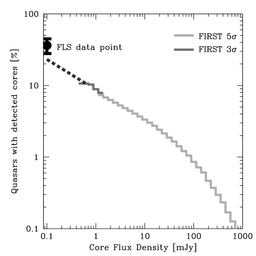
Figure 1: Plot of the fraction of quasars with a detected radio core as function of its flux density. The two lighter-grey curves are for the $5\sigma$ and $3\sigma$ catalogs respectively. The dashed dark-grey line represents an extrapolation of the expected number densities below our detection threshold. The limiting detection rates are: 9.2% ($5\sigma$), 11.8% ($3\sigma$), and 23.3% (extrapolation down to 0.1 mJy). The large dot represents the detection rate for the Spitzer First Look Survey (FLS) field ($36\pm 8$%). Matching is done within 3 arcseconds.

In this section, we quantify the fraction of quasars that exhibit core emission. We can actually go slightly deeper than the official FIRST catalog, with its nominal $5\sigma$ lower threshold of 1.0 mJy, by creating $3\sigma$ lists based on the radio images and quasar positions. This allows us to go down to a detection limit of $\sim 0.75$ mJy (versus 1.0 mJy for the official version).

Given the steeply rising number density distribution of radio sources toward lower flux levels, one might be concerned about the potential for an increase in false detections at sub-mJy flux density levels. The relative optical to radio astrometry is, however, accurate enough to match within small apertures (to better than 3″), reducing the occurrence of chance superpositions significantly. The surface density of radio sources at the 1 mJy level is not high enough to significantly contaminate the counts based on 3 arcsecond matching. The fraction of radio core detected quasars (RCDQ) out of the total quasar population hovers around the 10% mark, but this is a strong function of the radio flux density limit. It also depends on the initial selection of the quasar sample. The SDSS quasar selection is mainly done on their optical colors (Richards et al., 2002), but $\sim 3\%$ of the quasars were selected solely on the basis of their radio emission (1397 out of 44 984). Looking at only those SDSS quasars which have been selected expressly on their optical colors (see the quasar selection flow-chart of Richards et al. 2002, Fig 1), there are 34 147 sources which have either a QSO_CAP, QSO_SKIRT, and / or a QSO_HIZ flag set. For these, the relevant radio core detection fractions are 7.1% (2430) and 10.1% (3458) for the 5$\sigma$ and 3$\sigma$ detection limits, respectively (the binomial error on these percentages is on the order of 0.1%). These core fractions are higher for the 10 837 quasars (44 984$-$34 147) that made it into the SDSS sample via other means (1694, 15.6% and 1855, 17.1% for the 5 and 3$\sigma$ catalogs). The higher core fractions are due to the large number of targeted FIRST sources that would not have made it into the sample otherwise, and to the greater likelihood of radio emission among X-ray selected quasars. Clearly, the initial quasar selection criteria impact the rate at which their cores are detected by FIRST. The results have been summarized in Table 1.

A more direct view of the flux limit dependence of the RCDQ fraction is offered by Fig. 1. An extrapolation of the data suggests that at 0.1 mJy about 20% of quasar cores will be detected. This extrapolation is not unrealistic, and even may be an underestimate: the extragalactic Spitzer First Look Survey (FLS) field has been covered by both the SDSS and the VLA down to 0.1 mJy levels (Condon et al., 2003). Out of the 33 quasars in the DR3 that are covered by this VLA survey, we recover 12 using the exact same matching criterion. This corresponds to a fraction of 36%, which carries an 8% formal $1\sigma$ uncertainty.

In fact, judging by the progression of detection rate in Fig. 1, one does not have to go much deeper than 0.1 mJy to recover the majority of (optically) selected quasars. The results and discussion presented in this paper, however, are only relevant to the subset of quasars with cores brighter than $\sim 1$ mJy. It is this $\sim 10\%$ of the total that is well-sampled by the FIRST catalog. This should be kept in mind as well for the sections where we discuss radio quasar morphology.

3.2 Environment Matching

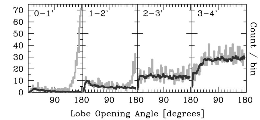
Figure 2: Histograms of lobe opening angles of FR2 quasar candidates. Each box represents a different FR2 size bin, as indicated by its diameter in arcminutes. The light-grey histogram represents the candidate count, and in dark-grey is the corresponding random-match baseline. This baseline increases dramatically as one considers larger sources, while the FR2 candidate count actually decreases. Note both the strong trend toward linear systems (180 degrees opening angles), as well as the significant presence of bent FR2 sources. The bin size 2.5 degrees.

The FIRST catalog is essentially a catalog of components, and not a list of sources. This means that sources which have discrete components, like the FR2 sources we are interested in, are going to have multiple entries in the FIRST catalog. If one uses a positional matching scheme as described in the last section, and then either visually or in an automated way assesses the quasar morphology, one will find a mix of core- and lobe-dominated quasars provided that the core has been detected. However, this mechanism is going to miss the FR2 sources without a detected core, thereby skewing the quasar radio population toward the core dominated sources.

Preferably one would like to develop an objective procedure for picking out candidate FR2 morphologies. We decided upon a catalog-based approach where the FIRST catalog was used to find all sources within a 450″ of a quasar position (excluding the core emission itself). Sources around the quasar position were then considered pairwise, where each pair was considered a potential set of radio lobes. Pairs were ranked by their likelihood of forming an FR2 based on their distances to the quasar and their opening angle as seen from the quasar position. Higher scores were given to opening angles closer to 180 degrees, and to smaller distances from the quasar. The most important factor turned out to be the opening angle. Nearby pairs of sources unrelated to the quasar will tend to have small opening angles as will a pair of sources within the same radio lobe of the quasar, so we weighted against candidate FR2 sources with opening angles smaller than 50°. The chances of these sources to be real are very small, and even if they are a single source, their relevance to FR2 sources will be questionable. We score the possible configurations as follows:

$$w_{i,j}=\frac{\Psi/50\arcdeg}{(r_{i}+r_{j})^{2}}$$ (1)

where $\Psi$ is the opening angle (in degrees), and $r_{i}$ and $r_{j}$ are the distance rank numbers of the components under consideration. The closest component to the quasar has an $r=0$, the next closest is $r=1$, etcetera. This way, the program will give the most weight to the radio components closest to the quasar, irrespective of what that separation turns out to be in physical terms. Each quasar which has at least 2 radio components within the 450″ search radius will get an assigned “most likely” FR2 configuration (i.e., the configuration with the highest score $w_{i,j}$. This, by itself, does not mean it is a real FR2.

In fact, this procedure turns up large numbers of false positives. Therefore, as a control, we searched for FR2 morphologies around a large sample of random sky positions that fall within the area covered by FIRST. Since all of the results for FR2s depend critically on the quality of the control sample, we increased this random sample size 20-fold over the actual quasar sample (of 44 984). Given the area of the FIRST survey ($\sim 9\,000$ sq. degree) and our matching area (1/20th of a sq. degree), a much larger number of pointings would start to overlap itself too much (i.e., the random samples would not be independent of each other).

In Fig. 2 we display a set of histograms for particular FR2 sizes. For each, the number FR2 candidates are plotted as a function of opening angle both around the true quasar position (light-grey trace) as well as the offset positions (dark-grey trace). There is a clear excess of nominal FR2 sources surrounding quasar positions which we take as a true measure of the number of quasars with associated FR2s. Although the distribution of FR2s has a pronounced peak at opening angles of 180 degrees, the distribution is quite broad, extending out to nearly 90 degrees. It is possible that some of this signal results from quasars living within (radio) clusters and hence being surrounded by an excess of unrelated sources, but such a signal should not show a strong preference for opening angles near 180 degrees.

The set of histograms also illustrates the relative importance of chance FR2 occurrences (dark-grey histograms), which become progressively more prevalent if one starts considering the larger FR2 configurations. While the smallest size bin does have some contamination ($\sim 14\%$ on average across all opening angles), almost all of the signal beyond opening angles of 90 degrees is real (less than 5% contamination for these angles). However, the significance of the FR2 matches drops significantly for the larger sources. More than 92% of the signal in the 3 to 4 arcminute bin is by chance. Clearly, most of the suggested FR2 configurations are spurious at larger diameter, and only deeper observations and individual inspection of a candidate source can provide any certainty.

In the next few sections we describe the results of the analysis.

4 Results

4.1 Fraction of FR2 quasars

The primary result we can quantify is the fraction of quasars that can be associated with a double lobed radio structure (whether a core has been detected in the radio or not). This is different from the discussion in § 3.1 which relates to the fraction of quasars that have radio emission at the quasar core position. This value, while considerably higher than the rates for the FR2 quasars, does not form an upper limit to the fraction of quasars associated with radio emission: some of the FR2 quasars do not have a detected radio core.

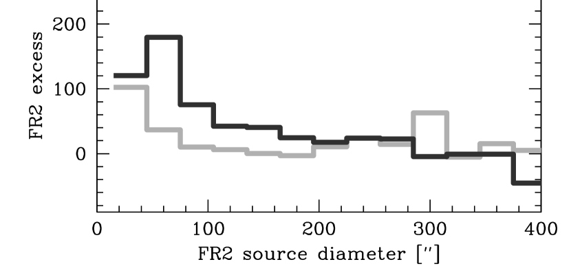
Figure 3: Number of excess FR2 candidates over the random baseline numbers as function of overall size. The histograms are for FR2 sources with cores (dark-grey) and without cores (light-grey). The summed excess counts within 300″ are 547 and 202 for the core and non-core subsamples, respectively. Note that the smallest size bin for the core sample is affected by resolution: it is hard to resolve a core inside a small double lobed structure.

Figure 2 depicts the excess number of FR2 quasars over the baseline values, plotted for progressively larger radio sources. The contamination rates go up as more random FIRST components fall within the covered area, and, at the same time, fewer real FR2 sources are found. This effect is illustrated in Fig. 3, which shows the FR2 excesses as function of overall source size. The light-grey line indicates the FR2 number counts for candidates without a detected (3$\sigma$) core, and the dark-grey histogram is for the FR2 candidates with a detected core. It is clear that FR2 sources larger than about 300″ are very rare, and basically cannot be identified using this method. Most FR2 sources are small, with the bulk being having diameters of less than 100″.

The summed total excess numbers, based on Fig. 3 and limited to 300″ or smaller, are 749 FR2 candidates (1.7% of the total), of which 547 have cores. Some uncertainties in the exact numbers still remain, particularly due to the noise in the counts at larger source sizes. A typical uncertainty of $\sim 20$ should be considered on these numbers (based on variations in the FR2 total using different instances of the random position catalog).

At these levels, it is clear that the FR2 phenomenon is much less common than quasar core emission; 1.7% versus 10% (see § 3.1). Indeed, of all the quasars with a detected radio core, only about 1 in 9 is also an FR2. The relative numbers have been recapitulated in Table 2.

4.2 Core Fractions of FR2 quasars

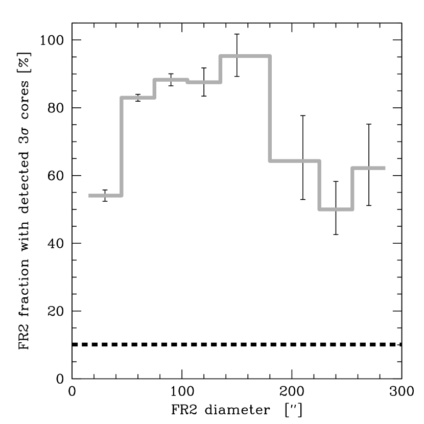
Figure 4: Fraction of FR2 sources that have detected ($>0.75$ mJy) cores, as function of overall size. As in Fig. 3, the smallest size bin is affected by the angular resolution of FIRST. The mean core fraction is 73.0%, which appears to be a representative value irrespective of the FR2 diameter The horizontal dashed line represents the core-fraction of the non-FR2 quasar population at 10.6%. The error estimates on the core fraction are a combination of binomial and background noise errors.

As noted above, not all FR2 quasars have cores that are detected by FIRST. We estimate that about 75% of FR2 sources have detected cores down to the 0.75 mJy flux density level. This value compares well with the number for our “actual” FR2 quasar sample of § 4.6. Out of 422 FR2 quasar sources, 265 have detected cores (62.8%) down to the FIRST detection limit (1 mJy).

We are now in the position of investigating whether there is a correlation between the overall size of the FR2 and the presence of a radio core. In orientation dependent unification schemes, a radio source observed close to the radio jet axis will be both significantly foreshortened and its core brightness will be enhanced by beaming effects (e.g., Barthel 1989, Hoekstra et al. 1997). This would imply that, given a particular distribution of FR2 radio source sizes and core luminosities, the smaller FR2 sources would be associated (on average) with brighter core components. This should translate into a higher fraction of detected cores among smaller FR2 quasars (everything else being equal). Figure 4 shows the fraction of FR2 candidates that have detected cores, as function of overall size. There does not appear to be a significant trend toward lower core-fractions as one considers larger sources. The much lower fraction for the very smallest size bin is due to the limited resolution of the FIRST survey (about 5″), which makes it hard to isolate the core from the lobe emission for sources with an overall size less than about half an arcminute. Also, beyond about 275″ the core-ratio becomes rather hard to measure; not a lot of FR2 candidates are this large (see Fig. 3).

Since the core-fraction is more or less constant, and does not depend on the source diameter, it does not appear that relativistic beaming is affecting the (faint) core counts. Unfortunately, one expects the strongest core beaming contributions for the smallest sources; exactly the ones that are most affected by our limited resolution.

4.3 Bent Double Lobed Sources

The angular distributions in Fig. 2 reveal a large number of more or less bent FR2 sources. Bends in FR2 sources can be due to a variety of mechanisms, either intrinsic or extrinsic to the host galaxy. Local density gradients in the host system can account for bending (e.g., Allan, 1984), or radio jets can run into overdensities in the ambient medium, resulting in disruption / deflection of the radio structure (e.g., Mantovani et al., 1998). Extrinsic bending of the radio source can be achieved through interactions with a (hot) intracluster medium. Any space motion of the source through this medium will result in ram-pressure bending of the radio structure (e.g., Soker et al., 1988; Sakelliou & Merrifield, 2000). And finally, radio morphologies can be severely deformed by merger events (e.g., Gopal-Krishna et al., 2003). Regardless of the possible individual mechanisms, a large fraction of our FR2 quasars have significant bending: only slightly more than 56% of FR2 quasars smaller than 3 arcminutes have opening angles larger than 170 degrees (this value is 65% for the actual sample of § 4.6). This large fraction of bent quasars is in agreement with earlier findings (based on smaller quasar samples) of, e.g., Barthel & Miley (1988); Valtonen et al. (1994); Best et al. (1995).

4.4 Redshift Correlations

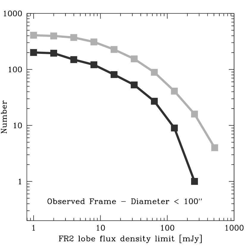
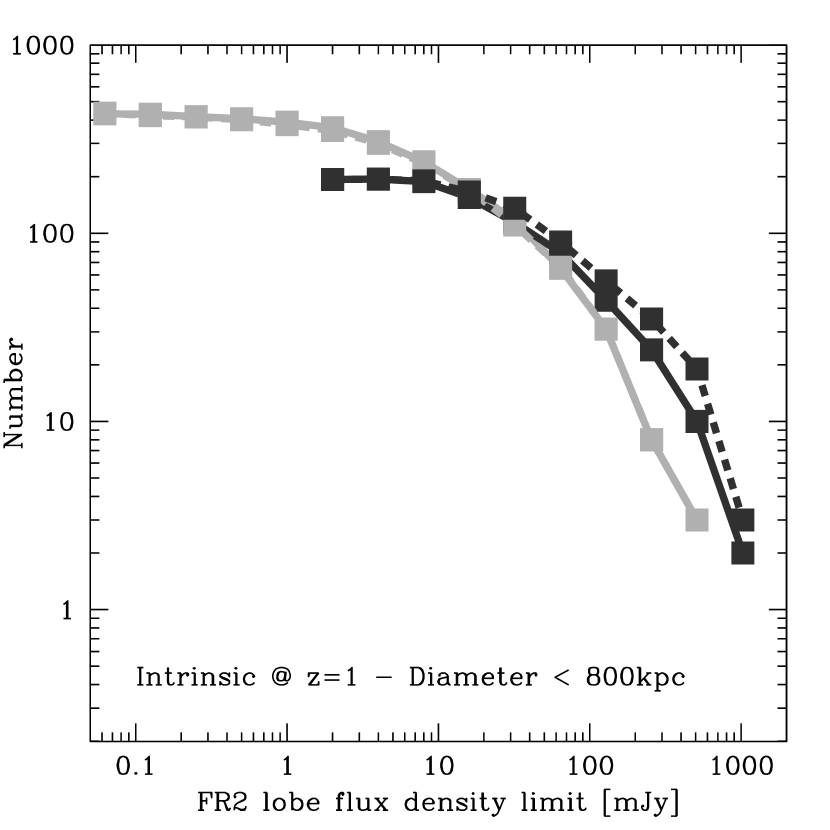
Figure 5: Cumulative number of FR2 candidates as function of a lower threshold to the lobe brightness. The left panel shows the distribution for the low-redshift (light-grey line) and high-redshift (dark-grey) halves of the sample. The flux limits are as observed (i.e., in mJy at 1.4GHz). There are about twice as many low-redshift FR2 candidates as high-redshift candidates. In the panel on the right the redshift dependencies have been taken out; all sources are placed on a fiduciary redshift of 1 by k-correcting their lobe flux densities. Note that the shape of the distribution only weakly depends on the assumed radio spectral index used in the k-correction (from $\alpha=0$ to the canonical radio spectral index of $\alpha=-0.75$, solid and dashed curves respectively).

We can investigate whether there are trends with quasar redshift based on statistical arguments. This is done by subdividing the sample of 44 984 in two parts (high and low redshift), and then comparing the results for each subsample. As with the main sample, each subsample has its own control sample providing the accurate baseline.

Previous studies (e.g., Blundell et al. 1999) have suggested that FR2 sources appear to be physically smaller at larger redshifts. For self-similar expansion the size of a radio source relates directly to its age. It also correlates with its luminosity, since, based on relative number densities of symmetric double lobed sources over a large range of sizes (e.g., Fanti et al. 1995, O’Dea & Baum 1997), one expects a significant decline in radio flux as a lobe expands adiabatically.

While the picture in a fixed flux density limit will preferentially bias against older (and therefore fainter) radio sources at higher redshifts, resulting in a “youth-size-redshift” degeneracy, scant hard evidence is available in the literature. Indeed, several studies contradict each other. See Blundell et al. (1999) for a nice summary. We, however, are in a good position to address this issue. First, our quasar sample has not been selected from the radio, and as such has perhaps less radio bias built in. Also, we have complete redshift information on our sample. The redshift range is furthermore much larger than in any of the previous studies. The median redshift for our sample of quasars is 1.3960, which results in mean redshifts for the low- and high-redshift halves of the sample of $\overline{z_{L}}=0.769$, and $\overline{z_{H}}=2.088$.

The first test we can perform on the 2 subsamples is to check whether their relative numbers as function of the average lobe flux density makes sense. The results are plotted in Fig. 5, left panel. The curves are depicting the cumulative number of FR2 candidates smaller than 100″ for which the mean lobe flux density is larger than a certain value. We have explicitly removed any core contribution to this mean. We limited our comparison here to the smaller sources, for which the background contamination is smallest.

Since the left panel shows the results in the observed frame, it is clear that we detect far more local FR2 sources than high redshift ones (light-grey curve in comparison to the dark-grey one). On average, more than twice as many candidates fall in the low-redshift bin compared to the high-redshift ones (408 candidates versus 201). Furthermore, the offset between the two curves appears to be fairly constant, indicating that the underlying population properties may not be that different (i.e., we can match both by shifting the high-redshift curve along the x-axis, thereby correcting for the lower lobe flux densities due to their larger distances). This is exactly what we have done in the right panel. All of the FR2 candidates have been put at a fiducial redshift of 1, correcting its lobe emission both for relative distances and intrinsic radio spectral index. For the former we assumed a WMAP cosmology (H${}_{\rm o}=71$ km s^-1 Mpc^-1, $\Omega_{\rm M}=0.3$, and $\Omega_{\Lambda}=0.7$), and for the latter we adopted $\alpha=-0.75$ for the high frequency part of the radio spectrum ($>1$ GHz). It should be noted that these cumulative curves are only weakly dependent on the cosmological parameters $\Omega$ and radio spectral index $\alpha$. It is not dependent on the Hubble constant. The physical maximum size for the FR2 candidates is set at 800kpc, which roughly corresponds to the 100″ size limit in the left panel.

Both curves agree reasonably well now. At the faint end of each curve, incompleteness of the FIRST survey flattens the distribution. This accounts for the count mismatch between the light- and dark-grey curves below about 10 mJy. On the other end of both curves, low number statistics increase the uncertainties. The slightly larger number of bright FR2 sources for the high-redshift bin (see Fig. 5, right panel) may be real (i.e., FR2 sources are brighter at high redshifts compared to their low-redshift counterparts), but the offset is not significant. Also note the effect of changing the radio spectral index from $-0.75$ to $0$ (dotted dark-grey line versus solid line). A negative $\alpha$ value has the effect of increasing the lobe fluxes, especially for the higher redshift sources. Flattening the $\alpha$ to $0$ (or toward even more unrealistic positive values) therefore acts to lower the average lobe fluxes, and as a consequence both cumulative distributions start to agree better. This would also suggest that the high-redshift sources may be intrinsically brighter, and that only by artificially lowering the fluxes can both distributions made to agree.

4.5 Physical FR2 sizes at low and high redshifts

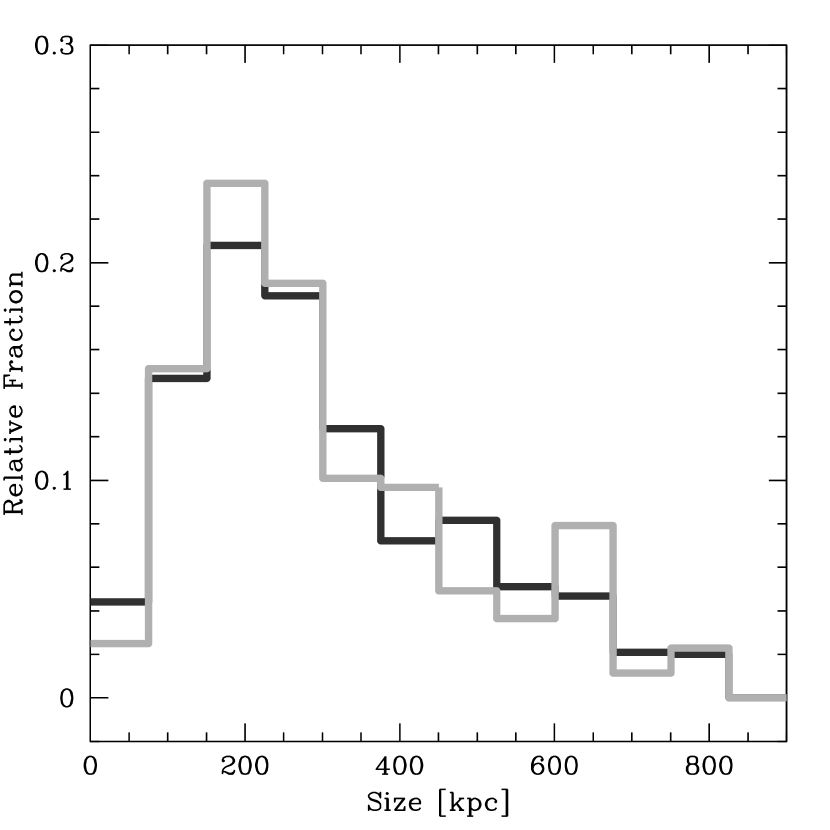
Figure 6: Histogram of the FR2 source size distribution. The light-grey histogram is for the low-redshift half of the sample, and the dark-grey line is for the high-redshift sources. Both histograms have been corrected for random matches, and therefore represent the real size distributions.

This brings us to the second question regarding redshift dependencies: are the high-redshift FR2 quasars intrinsically smaller because we are biased against observing older, fainter, and larger radio sources? To this end we used the same two datasets that were used for Fig. 5, right panel. The upper size limit is set at 800kpc for both subsets, but this does not really affect each size distribution, since there are not that many FR2 sources this large. Figure 6 shows both distributions for the low and high redshift bins (same coloring as before). As in Fig. 4, the smallest size bins are affected by resolution effects, albeit it is easier to measure the lobe separation than whether or not there is a core component between the lobes. The smallest FR2 sources in our sample are about 10″ ($\sim$80 kpc at $z=1$), which is a bit better than the smallest FR2 for which a clear core component can be detected ($\sim 30\arcsec$). The apparent peak in our size distributions (around 200 kpc) agrees with values found for 3CR quasars. Best et al. (1995) quote a value of $207\pm 29$ kpc, though given the shape of the distribution it is not clear how useful this measure is.

A Kolmogorov-Smirnoff test deems the difference between the low-redshift (green histogram) and high-redshift (blue histogram) size distributions insignificant. Therefore, it does not appear that there is evidence for FR2 sources to be smaller in the earlier universe.

An issue that has been ignored so far is that we tacitly assumed that the FR2 sizes for these quasars are accurate. If these sources have orientations preferentially toward our line of sight (and we are dealing with quasars here), significant foreshortening may underestimate their real sizes by quite a bit (see Antonucci 1993). This will also “squash” both distributions toward the smaller sizes, making it hard to differentiate the two.

Previous studies (e.g., Blundell et al., 1999) relied on (smaller) samples of radio galaxies, for which the assumption that they are oriented in the plane of the sky is less problematic. Other studies which mainly focused on FR2 quasars (e.g, Nilsson et al. 1998, Teerikorpi 2001) also do not find a size-redshift correlation.

4.6 Sample Specific Results

The next few sections deal with properties intrinsic to FR2 quasars. As such, we need a subsample of our quasar list that we feel consists of genuine FR2 sources. We know that out of the total sample of 44 984 about 750 are FR2 sources, however, we do not know which ones. What we can do is create a subsample that is guaranteed to have less than 5% of non-FR2 source contamination. This is done by stepping through the multidimensional space spanned up by histograms of the Fig. 2 type as function of overall size. As can be seen in Fig. 2, the bins with large opening angles only have a small contamination fraction (in this case for sources smaller than 100″). Obviously, the signal-to-noise goes down quite a bit for larger overall sizes, and progressively fewer of those candidates are real FR2. By assembling all the quasars in those bins that have a contamination rate less than 5%, as function of opening angle and overall size, we constructed a FR2 quasar sample that is more reliable than 95%. It contains 422 sources, and forms the basis for our subsequent studies. Sample properties are listed in Table 3, and the positions of the 417 actual FR2 quasars are given in Table 4.

4.7 FR2 Sample Asymmetries

The different radio morphological properties of the FR2 sources have been used with varying degrees of success to infer its physical properties. In particular, these are: the observed asymmetries in the arm-length ratio ($Q$, here defined as the ratio of the larger lobe-core to the smaller lobe-core separation), the lobe flux density ratio ($F=F_{\rm lobe,distant}/F_{\rm lobe,close}$), and the distribution of the lobe opening angle ($\Psi$, with a linear source having a $\Psi$ of 180°).

Gopal-Krishna & Wiita (2004) provide a nice historic overview of the literature on these parameters. As can be inferred from a median flux ratio value of $F<1.0$ (see Table 5), the closer lobe is also the brightest. This is consistent with the much earlier findings of Mackay (1971) for the 3CR catalog, and implies directly that the lobe advance speeds are not relativistic, and that most of the arm-length and flux density asymmetries are intrinsic to the source (and not due to orientation, relativistic motions, and Doppler boosting).

If we separate the low and high-redshift parts of our sample, we can test whether any trend with redshift appears. Barthel & Miley (1988), for instance, suggested that quasars are more bent at high redshifts. In our sample we do not find a strong redshift dependency. The median opening angles are 173.6 and 172.7°, for the low and high redshift bins respectively. A Kolmogorov-Smirnoff test deemed the two distributions different at the 97.2% confidence level (a 2.2$\sigma$ results). This would marginally confirm the Barthel & Miley claim. However, Best et al. (1995) quote a 2$\sigma$ result in the opposite sense, albeit using a much smaller sample (23 quasars).

We also found no significant differences between the low and high-redshift values of the arm-length ratios $Q$ (KS-results: different at the 87.0% level, 1.51$\sigma$), and the flux ratios $F$ (similar at the 97.0% level, 2.2$\sigma$).

The Mackay-type asymmetry, in which the nearest lobe is also the brightest, is not found to break down for the brightest of our quasars. If we separate our sample into a low- and high-flux bin (which includes the core contribution), we do not see a reversal in the flux asymmetry toward the most radio luminous FR2 sources (e.g., Gopal-Krishna & Wiita, 2004, and references therein). Actually, for our sample we find a significant (3.25$\sigma$) trend for the brightest quasars to adhere more to the Mackay-asymmetry than the fainter ones.

4.8 Control Samples

Using the same matching technique as described in the previous section, we made two additional control samples. Whereas our FR2 sample is selected based on a combination of large opening angle ($\gtrsim 150$ degrees) and small overall size ($\lesssim 200$″), our control samples form the other extreme. Very few, if any, genuine FR2 sources will be characterized by radio structures with small opening angles ($<100$ degrees) and large sizes ($>450$″). Therefore, we use these criteria to select two non-FR2 control samples: one that has a FIRST source coincident with the quasar (remember that the matching algorithm explicitly excludes components within 3″ of the quasar position), and another one without a FIRST counterpart to the quasar. For all practical purposes, we can consider the former sample to be quasars which are associated with just one FIRST component (the “core dominated” sample - CD), and the latter as quasars without any detected FIRST counterpart (the “radio quiet” sample - RQ).

Both of the CD and RQ samples initially contained more candidates than the FR2 sample. This allows for small adjustments in the mean sample properties, in particular the redshift distribution. We therefore matched the redshift distribution of the CD and RQ samples to the one of the FR2 sample. This resulted in a CD sample which matches the FR2 in redshift-space and in absolute number. The RQ sample, which will function as a baseline to both the FR2 and CD samples, contains a much larger number (6330 entries), but again with an identical redshift distribution. The mean properties of the samples are listed in Table 3.

4.9 Composite Optical Spectra

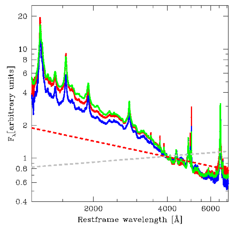
Figure 7: Composite spectra for our three samples of quasars: radio quiet (RQ) quasars in green, core dominated (CD) radio-loud quasars in blue, and lobe dominated (FR2) radio-loud quasars in red. This plot can be directly compared to Fig. 7 of Richards et al. (2003), and illustrates both the small relative color range among our 3 samples (all fall within the “normal” range of Richards et al.), and the apparent lack of significant intrinsic dust-reddening in these quasars (the red and gray dashed lines represent moderate to severe levels of dust-reddening). All spectra have been normalized to the continuum flux at 4000Å.

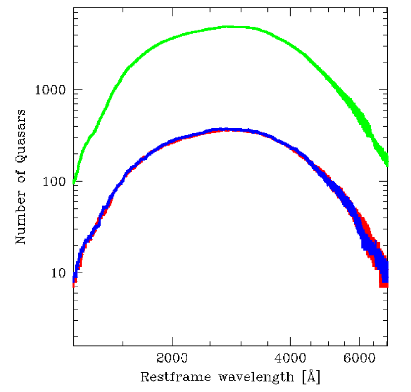
Figure 8: Number of quasars that contributed to the composite spectrum as function of wavelength. The color-coding is the same as for Fig. 7. The RQ sample (green histogram) contains 15 times as many quasars as both the CD and FR2 samples.

One of the very useful aspects of our SDSS based quasar sample is the availability of a large set of complementary data, including the optical spectra for all quasars. An otherwise almost impossible stand-alone observing project due to the combination of low FR2 quasar incidence rates and large datasets, is sidestepped by using the rich SDSS data archive. We can therefore readily construct composite optical spectra for our 3 samples (as listed in Table 3). We basically used the same method for the construction of the composite spectrum as outlined by vanden Berk et al. (2001), in combination with a relative normalization scheme similar to the ones used in Richards et al. (2003). Each composite has been normalized by its continuum flux at 4000Å (restframe).

The resulting spectra are plotted in Fig. 7, color coded green for the radio-quiet (RQ) quasar control sample, blue for the core-dominated (CD) radio-loud quasars, and red for the lobe dominated (FR2) radio quasars. All three composite spectra are similar to each other and to the composite of vanden Berk et al. (2001). Figure 8 shows the number of quasars from each subsample that were used in constructing the composite spectrum. Since each individual spectrum has to be corrected by a $(1+z)$ factor to bring it to its restframe, not all quasars contribute to the same part of the composite. In fact, the quasars that contribute to the shortest wavelengths are not the same that go into the longer wavelength part. This should be kept in mind if one wants to compare the various emission lines. Any dependence of the emission line properties on redshift will therefore affect the short wavelength part of the composite more than the long wavelength part (which is made up of low redshift sources).

Richards et al. (2003) investigated the effect of dust-absorption on composite quasar spectra (regardless of whether they are associated with radio sources), and we have indicated two of the absorbed template spectra (composite numbers 5 and 6, see their Fig. 7) in our Fig. 7 as the red and gray dashed lines, respectively. From this it is clear that our 3 sub-samples do not appear to have significant intrinsic dust-absorption associated with them. Indeed, the range of relative fluxes toward the blue end of the spectrum falls within the range of “normal” quasars (templates 1$-$4 of Richards et al. (2003)). The differences in spectral slopes among our 3 samples are real. We measure continuum slopes (over the range 1450 to 4040Å, identical to Richards et al. (2003)) of: $\alpha_{\nu}=-0.59\pm 0.01$, $\alpha_{\nu}=-0.47\pm 0.01$, and $\alpha_{\nu}=-0.80\pm 0.01$ for the FR2, RQ, and CD samples respectively. These values are significantly different from the reddened templates ($\alpha_{\nu}=-1.51$ and $\alpha_{\nu}=-2.18$ for the red and grey dashed lines in Fig. 7), suggesting that our quasars are intrinsically different from dust-reddened quasars (e.g., Webster et al., 1995; Francis et al., 2000).

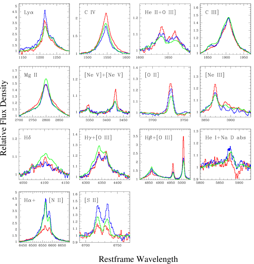
Figure 9: Composite spectra of the three comparison samples, centered around emission line regions. The histograms are color-codes as follows: green is for the radio quiet (RQ) quasar population, the blue for the core dominated (CD) sample, and red represents the lobe dominated FR2 quasars. All the spectra have been normalized to the continuum flux levels at the left and right parts of each panel.

In order to study differences in line emission, small differences in spectral slope have to be removed. This is achieved by first normalizing each spectrum to the continuum flux just shortward of the emission line in question. Then, by fitting a powerlaw to the local continuum, each emission line spectrum can be “rectified” to a slope of unity (i.e., making sure both the left and right sides of the zoomed-in spectrum are set to unity). A similar approach has been employed by Richards et al. (2003, see their Figs. 8 and 9).

The results are plotted in Fig. 9, zoomed in around prominent emission lines. The panels are arranged in order of increasing restframe wavelength. A few key observations can be made. The first, and most striking one, is that FR2 quasars tend to have stronger moderate-to-high ionization emission lines in their spectrum than either the CD and RQ samples. This can be seen especially for the C IV, [Ne V], [Ne III], and [O III] emission lines. The inverse appears to be the case for the Balmer lines: the FR2 sources have significantly fainter Balmer lines than either the CD or RQ samples. Notice, for instance, the H$\delta$, H$\gamma$, H$\beta$, and H$\alpha$ sequence in Fig. 9. Other lines, like Mg II and C III], do not seem to differ among our 3 samples.

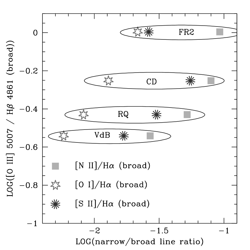
Figure 10: Relative importance of broad versus narrow emission lines in our 3 subsamples. For comparison, we included ratios taken from Vanden Berk et al. (2001), based on a sample of $\sim 2000$ quasars. Datapoints in the lower left corner can be considered dominated by the broad line component, whereas a point in the upper right has a more substantial narrow line contribution. The trend for the FR2 sample to be the one that is most dominated by line emission is apparent, and consistent for various ratios (as indicated).

Measured line widths, line centers and fluxes for the most prominent emission lines are listed in Table 6. Since a lot of the lines have shapes that are quite different from the Gaussian form, we have fitted the profiles with the more general form $F(x)=ce^{-0.5(x/\sigma)^{n}}$, with $c$ a normalization constant, and $n$ a free parameter. Note that for a Gaussian, $n=2$. The FWHM of the profile can be obtained directly from the values of $n$ and $\sigma$: $\mbox{FWHM}=2(2ln2)^{1/n}\sigma$. Allowing values of $n<2$ results in better fits for lines with broad wings (e.g., C III$]$ in Fig. 9). Typically the difference in equivalent width (EW) as fitted by the function and the actual measured value is less than 1%. The fluxes in Table 6 have been derived from the measured EW values, multiplied by the continuum level at the center of the line (as determined by a powerlaw fit, see Fig. 7). Since all composite spectra have been normalized to a fiducial value of 1.00 at 4000Å  the fluxes are relative to this 4000Å continuum value, and can be compared across the three samples (columns 6 and 11 in Table 6). In addition, we have normalized these fluxes by the value of the Ly$\alpha$ flux for each subsample. This effectively takes out the slight spectral slope dependency, and allows for an easier comparison to the values of vanden Berk et al. (2001, their Table 2).

The differences between the various species of emission lines among the 3 subsamples, as illustrated in Fig. 9, are corroborated by their line fluxes and ratios. Even though we cannot use emission line ratios (like $[$O I$]$ / H$\alpha$, see Osterbrock 1989) to determine whether we are dealing with AGN or H II-region dominated emission regimes (due to the fact that the broad and narrow lines do not originate from the same region), we can still discern trends between the subsamples in the relative importance of broad vs. narrow line emission. This is illustrated by Fig. 10, in which we have plotted various ratios of narrow and broad emission lines (based on fluxes listed in Table 6). The narrow lines are normalized on the $x$-axis by the broad-line H$\alpha$ flux, and on the $y$-axis by the broad-line component (listed separately in Table 6) of the H$\beta$ line. It is clear from this plot that, as one progresses from RQ, CD, to FR2 sample, the relative importance of various narrow lines increases. The offset between the RQ and Vanden Berk samples (which in principle should coincide) is in part due to the presence of a narrow-line component in their H$\beta$ fluxes (lowering the points along the $y$-axis), and a slightly larger flux density in their composite H$\alpha$ line (moving the points to the left along the $x$-axis). The offset probably serves best to illustrate the inherent uncertainties in plots like these.

So, in summary, it appears that the FR2 sources tend to have brighter moderate-to-high ionization lines, while at the same time having much less prominent Balmer lines, than either the CD or RQ samples. The latter two have far stronger comparable emission line profiles / fluxes, with the possible exception of the higher Balmer lines and [S II].

Radio sources are known to interact with their ambient media, especially in the earlier stages of radio source evolution where the structure is confined to within the host galaxy. In these compact stages, copious amounts of line-emission are induced at the interfaces of the radio plasma and ambient medium (e.g., Bicknell et al., 1997; de Vries et al., 1999; Axon et al., 1999). Other types of radio activity related spectral signatures are enhanced star-formation induced by the powerful radio jet (e.g., van Breugel et al., 1985; McCarthy et al., 1987; Rees, 1989), scattered nuclear UV light off the wall of the area “excavated” by the radio structure (e.g., di Serego Alighieri et al., 1989; Dey et al., 1996), or more generally, direct photo-ionization of the ambient gas by the AGN along radiation cones coinciding with the radio symmetry axis (e.g., Neeser et al., 1997). The last three scenarios are more long-lived (i.e., the resulting stars will be around for a while), whereas the shock-ionization of the line emission gas is an in-situ event, and will only last as long as the radio source is there to shock the gas ($<10^{6}$ years).

It therefore appears reasonable to guess that in the case of the FR2 quasars, such an ongoing interaction between the radio structure and its ambient medium is producing the excess flux in the narrow lines. Indeed, shock precursor clouds are found to be particularly bright in high-ionization lines like $[$O III$]$ compared to H$\alpha$ (e.g., Sutherland et al., 1993; Dopita & Sutherland, 1996). Since the optical spectrum is taken at the quasar position, and not at the radio lobe position, we are obviously dealing with interactions between the gaseous medium and the radio core (whether we detected one or not).

The other sample of quasars associated with radio activity, the core-dominated (CD) sample, has optical spectral properties which do not differ significantly from radio-quiet quasars.

5 Summary and Conclusions

We have combined a sample of 44 984 SDSS quasars with the FIRST radio survey. Instead of comparing optical and radio positions for the quasars directly to within a small radius (say, 3″), we matched the quasar position to its complete radio environment within 450″. This way, we are able to characterize the radio morphological make-up of what is essentially an optically selected quasar sample, regardless of whether the quasar (nucleus) itself has been detected in the radio.

The results can be separated into ones that pertain to the quasar population as a whole, and those that only concern FR2 sources. For the former category we list: 1) only a small fraction of the quasars have radio emission associated with the core itself ($\sim 11\%$ at the 0.75 mJy level); 2) FR2 quasars are even rarer, only 1.7% of the general population is associated with a double lobed radio source; 3) of these, about three-quarter have a detected core; 4) roughly half of the FR2 quasars have bends larger than 20 degrees from linear, indicating either interactions of the radio plasma with the ICM or IGM; and 5) no evidence for correlations with redshift among our FR2 quasars was found: radio lobe flux densities and radio source diameters of the quasars have similar distributions at low and high redshifts.

To investigate more detailed source related properties, we used an actual sample of 422 FR2 quasars and two comparison samples of radio quiet and non-FR2 radio loud quasars. These three samples are matched in their redshift distributions, and for each we constructed an optical composite spectrum using SDSS spectroscopic data. Based on these spectra we conclude that the FR2 quasars have stronger high-ionization emission lines compared to both the radio quiet and non-FR2 radio loud sources. This may be due to higher levels of shock ionization of the ambient gas, as induced by the expanding radio source in FR2 quasars.

Table 1: Radio Core Matching

	Number	($5\sigma$ matches)	($3\sigma$ matches)
SDSS Optically Selected	34 147	2430 (7.1%)	3458 (10.1%)
SDSS Otherwise Selected	10 837	1694 (15.6%)	1855 (17.1%)
Total	44 984	4124 (9.2%)	5313 (11.8%)

Table 2: Relative Makeup of Quasar Sample

Total number of quasars	44 984	Fraction
Quasars with detected cores (3$\sigma$ limit)	5 313	11.8%
Non-FR2 quasars with detected cores	4 766	10.6%
FR2 quasars	749	1.7%
FR2 quasars with detected core	547	73%
FR2 quasars without core	202	27%

Table 3: Redshift Matched Subsamples - Properties

	FR2 sample	CD sample	RQ sample
Sample Size	422	422	6330
$u$-band	19.41$\pm$0.05	19.69$\pm$0.06	19.61$\pm$0.01
$g$-band	19.11$\pm$0.11	19.29$\pm$0.05	19.33$\pm$0.01
$r$-band	18.88$\pm$0.04	18.98$\pm$0.05	19.14$\pm$0.01
$i$-band	18.74$\pm$0.04	18.78$\pm$0.05	19.01$\pm$0.01
$z$-band	18.64$\pm$0.04	18.68$\pm$0.05	18.94$\pm$0.01
Redshift	1.196$\pm$0.026	1.206$\pm$0.027	1.209$\pm$0.007

Table 4: FR2 Quasar Sample

Optical Positions (J2000)
00 03 45.23 $-$11 08 18.7	00 11 38.44 $-$10 44 58.2	00 43 23.43 $-$00 15 52.6	00 44 13.73 $-$00 51 41.0	00 51 15.12 $-$09 02 08.5
00 55 08.55 $-$10 52 06.2	00 59 29.12 $-$10 17 35.0	01 03 29.43 $-$00 40 55.1	01 17 49.91 $-$09 05 54.6	01 48 47.61 $-$08 19 36.3
02 35 30.71 $-$07 05 04.5	02 40 55.56 $-$00 12 01.2	02 48 02.56 $-$07 19 15.8	02 50 48.67 $-$00 02 07.6	02 55 12.17 $-$00 52 24.5
03 03 35.76 $-$00 41 45.0	03 04 58.97 $-$00 02 35.7	03 12 26.12 $-$00 37 08.9	03 13 18.66 $-$00 36 23.8	07 34 28.88 $-$32 50 58.4
07 41 00.60 $-$39 55 59.5	07 41 25.22 $-$33 33 20.1	07 42 42.19 $-$37 44 02.1	07 44 51.37 $-$29 20 06.0	07 45 41.67 $-$31 42 56.7
07 48 32.24 $-$26 34 38.9	07 49 37.69 $-$38 04 43.4	07 52 05.91 $-$28 02 10.8	07 52 06.74 $-$24 51 18.8	07 52 28.56 $-$37 50 53.6
07 54 04.24 $-$42 58 04.3	07 55 37.03 $-$25 42 39.0	07 56 25.82 $-$25 09 21.6	07 56 43.10 $-$31 02 48.8	07 59 58.76 $-$25 04 38.4
08 00 52.64 $-$41 57 38.8	08 01 29.58 $-$46 26 22.8	08 01 39.94 $-$31 53 29.8	08 02 20.52 $-$30 35 43.0	08 02 50.86 $-$33 35 17.8
08 05 55.67 $-$34 41 32.3	08 06 44.41 $-$48 41 49.2	08 08 33.37 $-$42 48 36.4	08 10 02.06 $-$26 03 40.5	08 11 36.90 $-$28 45 03.6
08 11 37.23 $-$48 31 33.8	08 13 18.85 $-$50 12 39.8	08 14 09.22 $-$32 37 32.0	08 15 40.84 $-$39 54 37.8	08 18 38.88 $-$43 17 55.6
08 20 50.76 $-$40 34 56.6	08 21 17.15 $-$48 45 46.3	08 21 25.97 $-$51 37 15.6	08 21 33.61 $-$47 02 37.3	08 22 14.18 $-$30 54 37.8
08 23 25.27 $-$44 58 50.5	08 26 16.35 $-$52 12 09.3	08 30 31.93 $-$05 20 06.8	08 31 36.99 $-$30 48 26.8	08 32 36.34 $-$33 31 54.7
08 34 44.62 $-$34 04 14.4	08 38 40.58 $-$47 34 10.7	08 39 23.24 $-$06 09 58.9	08 42 52.40 $-$44 34 10.6	08 43 52.87 $-$37 42 28.3
08 47 02.79 $-$01 30 01.4	08 49 25.89 $-$56 41 32.2	08 50 39.95 $-$54 37 53.4	08 51 14.93 $-$01 59 53.2	08 52 00.44 $-$02 29 34.5
08 52 32.83 $-$38 36 56.1	08 53 41.19 $-$40 52 21.8	09 01 02.73 $-$42 07 46.4	09 02 07.20 $-$57 07 37.9	09 02 21.53 $-$48 11 36.5
09 02 29.23 $-$48 39 06.2	09 04 36.36 $-$51 07 28.2	09 05 01.56 $-$53 39 07.5	09 05 13.17 $-$42 24 51.9	09 06 00.09 $-$57 47 30.1
09 07 45.47 $-$38 27 39.1	09 08 08.80 $-$00 35 00.5	09 08 12.17 $-$51 47 00.8	09 08 21.02 $-$04 50 59.5	09 10 17.33 $-$37 42 52.1
09 12 05.16 $-$54 31 41.3	09 15 28.77 $-$44 16 32.9	09 17 18.68 $-$59 03 40.4	09 17 57.43 $-$02 37 34.0	09 18 43.09 $-$40 17 09.7
09 19 21.56 $-$50 48 55.4	09 22 25.14 $-$43 07 49.4	09 23 08.17 $-$56 14 55.4	09 23 13.54 $-$04 34 45.0	09 24 54.56 $-$49 18 04.2
09 28 37.98 $-$60 25 21.0	09 28 56.83 $-$07 36 19.0	09 31 38.29 $-$03 15 10.1	09 35 18.19 $-$02 04 15.5	09 35 53.82 $-$05 03 53.2
09 36 28.68 $-$01 23 29.3	09 41 04.01 $-$38 53 51.0	09 41 24.74 $-$03 39 16.4	09 41 32.54 $-$02 04 32.6	09 41 44.82 $-$57 51 23.7
09 42 03.05 $-$54 05 18.9	09 43 58.22 $-$02 26 30.6	09 44 38.79 $-$08 51 57.0	09 47 40.01 $-$51 54 56.8	09 51 26.48 $-$01 46 51.8
09 52 28.46 $-$06 28 10.5	09 52 45.57 $-$00 00 15.5	09 55 56.38 $-$06 16 42.5	09 58 02.82 $-$44 06 03.7	10 00 54.68 $-$53 32 06.0
10 03 11.56 $-$50 57 05.2	10 03 50.71 $-$52 53 52.2	10 05 07.08 $-$50 19 29.6	10 06 33.64 $-$44 35 00.7	10 09 43.56 $-$05 29 53.9
10 10 27.52 $-$41 32 39.1	10 11 35.45 $-$00 57 43.1	10 12 54.25 $-$61 36 34.6	10 13 28.77 $-$07 56 53.8	10 15 41.14 $-$59 44 45.4
10 16 09.93 $-$45 31 43.2	10 16 51.74 $-$00 33 47.0	10 21 06.04 $-$45 23 31.9	10 22 35.57 $-$45 41 05.5	10 23 20.89 $-$01 02 27.5
10 26 31.97 $-$06 27 33.0	10 27 06.26 $-$06 09 59.2	10 27 25.96 $-$52 26 37.0	10 30 24.95 $-$55 16 22.8	10 31 43.51 $-$52 25 35.2
10 33 51.88 $-$00 24 14.3	10 34 18.01 $-$08 36 26.7	10 38 38.82 $-$49 47 36.9	10 39 36.67 $-$07 14 27.4	10 41 12.53 $-$00 45 49.3
10 42 07.56 $-$50 13 22.0	10 43 12.84 $-$00 13 49.1	10 45 34.98 $-$00 55 29.5	10 45 49.00 $-$53 47 59.8	10 47 26.65 $-$01 11 47.5
10 47 40.47 $-$02 07 57.3	10 49 32.22 $-$05 05 31.7	10 51 41.17 $-$59 13 05.2	10 53 10.16 $-$58 55 32.8	10 53 52.87 $-$00 58 52.8
10 54 54.97 $-$06 14 53.1	10 54 57.04 $-$00 45 53.0	10 55 00.34 $-$52 02 00.9	10 55 17.27 $-$02 05 45.1	10 56 54.16 $-$05 17 13.3
10 57 51.58 $-$02 27 40.9	11 05 14.28 $-$01 09 08.2	11 07 09.51 $-$05 47 44.8	11 07 15.89 $-$05 33 06.7	11 07 18.88 $-$10 04 17.7
11 07 45.78 $-$60 09 13.9	11 12 14.45 $-$01 20 48.5	11 12 17.48 $-$61 49 26.5	11 17 08.86 $-$00 43 10.6	11 17 16.60 $-$57 58 11.8
11 17 40.84 $-$05 28 58.7	11 20 48.50 $-$03 32 47.1	11 24 11.66 $-$03 37 04.7	11 25 06.96 $-$00 16 47.6	11 27 13.99 $-$01 11 53.3
11 30 44.30 $-$01 37 24.6	11 32 35.86 $-$01 28 48.7	11 32 50.84 $-$00 20 01.0	11 33 03.03 $-$00 15 48.9	11 33 25.15 $-$55 11 24.4
11 36 04.92 $-$52 25 58.9	11 37 03.09 $-$01 40 06.3	11 37 23.46 $-$02 15 08.2	11 41 11.62 $-$01 43 06.7	11 43 12.04 $-$53 50 48.3
11 44 33.67 $-$60 15 38.9	11 45 10.39 $-$01 10 56.3	11 47 34.30 $-$04 30 47.3	11 48 47.83 $-$10 54 58.4	11 49 18.97 $-$02 39 26.2
11 51 44.39 $-$52 44 12.6	11 54 05.38 $-$56 20 40.9	11 54 09.28 $-$02 38 15.0	11 56 51.58 $-$05 03 35.7	11 58 39.92 $-$62 54 27.9
11 59 23.69 $-$01 52 24.2	11 59 40.97 $-$01 27 08.5	12 05 17.33 $-$00 29 56.9	12 07 08.02 $-$02 44 44.1	12 09 49.98 $-$54 26 31.6
12 11 28.87 $-$50 52 54.2	12 11 54.87 $-$60 44 26.1	12 15 29.56 $-$53 35 55.9	12 15 41.96 $-$05 19 32.6	12 15 57.60 $-$00 07 19.8
12 17 01.37 $-$10 19 52.9	12 18 58.76 $-$01 52 37.9	12 20 27.98 $-$09 28 27.3	12 20 49.15 $-$58 59 21.6	12 21 30.39 $-$02 41 33.0
12 31 24.11 $-$01 12 07.3	12 36 23.80 $-$06 02 08.2	12 36 33.12 $-$10 09 28.7	12 37 53.86 $-$00 16 37.8	12 38 29.96 $-$00 13 27.9
12 40 00.93 $-$03 40 51.6	12 41 16.49 $-$51 41 30.0	12 41 39.73 $-$49 34 05.5	12 41 57.55 $-$63 32 41.6	12 42 16.38 $-$00 47 43.7
12 44 47.32 $-$59 41 07.4	12 45 38.35 $-$55 11 32.7	12 47 10.29 $-$55 55 57.3	12 47 58.52 $-$62 50 49.3	12 51 51.03 $-$49 18 55.0
12 53 11.26 $-$01 20 27.3	12 54 02.16 $-$00 49 31.1	12 55 08.10 $-$62 20 50.5	12 55 28.30 $-$00 54 42.0	12 55 54.74 $-$57 54 25.4
12 57 03.12 $-$00 24 36.0	12 57 29.79 $-$01 32 39.6	12 57 37.07 $-$00 32 20.2	12 58 24.70 $-$02 08 46.8	12 59 45.18 $-$03 17 26.2
13 02 10.16 $-$05 08 15.2	13 05 21.33 $-$49 51 42.3	13 08 28.73 $-$50 26 23.2	13 08 42.88 $-$02 43 26.7	13 09 07.99 $-$52 24 37.3
13 10 28.51 $-$00 44 08.9	13 10 40.56 $-$03 34 12.0	13 10 40.74 $-$02 01 27.1	13 15 38.72 $-$01 58 46.2	13 16 00.79 $-$02 18 19.6
13 16 14.50 $-$02 39 38.8	13 17 26.13 $-$02 31 50.5	13 18 27.00 $-$62 00 36.3	13 25 09.70 $-$00 49 33.9	13 26 07.16 $-$47 54 41.5
13 26 31.45 $-$47 37 55.9	13 26 55.72 $-$02 07 27.4	13 27 46.16 $-$48 42 03.0	13 29 09.25 $-$48 01 09.7	13 32 21.85 $-$53 28 17.4
13 32 59.17 $-$49 09 46.8	13 34 11.70 $-$55 01 25.0	13 34 37.49 $-$56 31 47.9	13 38 02.81 $-$42 39 57.0	13 39 48.45 $-$47 41 17.1
13 40 42.88 $-$02 03 07.5	13 40 48.37 $-$43 33 59.9	13 41 34.85 $-$53 44 43.7	13 45 45.36 $-$53 32 52.3	13 46 17.55 $-$62 20 45.5
13 47 39.84 $-$62 21 49.6	13 50 54.59 $-$05 22 06.5	13 52 23.24 $-$48 46 12.2	13 53 05.54 $-$04 43 38.7	13 54 09.95 $-$01 41 50.7
13 57 03.83 $-$02 30 07.1	13 58 23.52 $-$60 25 07.3	13 59 53.80 $-$59 11 03.0	13 59 59.08 $-$01 44 54.2	14 01 30.69 $-$41 55 15.3
14 02 14.80 $-$58 17 46.8	14 05 18.48 $-$04 34 06.9	14 06 56.49 $-$46 17 12.5	14 08 32.48 $-$47 38 37.4	14 08 32.65 $-$00 31 38.5
14 10 30.99 $-$61 41 37.0	14 10 54.06 $-$58 46 55.4	14 11 23.51 $-$00 42 53.0	14 12 31.18 $-$54 55 11.5	14 15 32.19 $-$40 49 51.6
14 17 08.16 $-$46 07 05.4	14 17 40.03 $-$60 53 23.8	14 19 32.59 $-$00 31 20.3	14 20 33.26 $-$00 32 33.3	14 21 27.77 $-$58 47 57.6
14 22 35.89 $-$01 52 11.2	14 24 14.09 $-$42 14 00.1	14 26 06.19 $-$40 24 32.0	14 27 45.71 $-$55 04 10.3	14 27 46.79 $-$00 28 44.7
14 28 29.93 $-$44 39 49.7	14 30 17.34 $-$52 17 35.1	14 32 44.44 $-$00 59 15.1	14 33 39.38 $-$50 52 26.9	14 34 10.77 $-$01 23 41.7
14 36 27.37 $-$52 14 00.0	14 37 56.93 $-$01 56 38.9	14 38 06.25 $-$00 35 34.8	14 38 20.93 $-$02 39 53.1	14 38 34.54 $-$39 42 60.0
14 39 39.95 $-$44 28 51.0	14 40 01.64 $-$61 01 33.9	14 43 34.57 $-$02 19 26.5	14 44 14.21 $-$43 36 55.5	14 46 36.90 $-$00 46 56.5
14 47 07.41 $-$52 03 40.1	14 48 14.94 $-$57 41 45.7	14 50 49.93 $-$00 01 44.4	14 51 34.61 $-$01 59 37.0	14 52 40.92 $-$43 08 14.3
14 52 47.37 $-$47 35 29.2	15 00 07.27 $-$56 36 00.8	15 00 31.81 $-$48 36 46.8	15 01 21.97 $-$01 44 01.2	15 04 05.11 $-$46 28 51.3
15 04 31.30 $-$47 41 51.3	15 05 45.05 $-$41 17 26.7	15 08 24.74 $-$56 04 23.3	15 08 35.94 $-$60 32 58.6	15 09 40.59 $-$60 38 21.3
15 11 09.22 $-$56 50 51.8	15 12 15.74 $-$02 03 17.0	15 13 25.62 $-$42 00 16.8	15 13 34.31 $-$46 12 57.7	15 13 56.16 $-$04 20 55.8
15 14 15.96 $-$57 49 04.0	15 15 03.23 $-$61 35 20.1	15 19 36.72 $-$53 42 55.5	15 20 21.04 $-$02 53 12.1	15 20 25.64 $-$59 39 55.4
15 23 46.79 $-$02 22 39.5	15 25 05.36 $-$53 06 22.9	15 26 03.80 $-$58 25 25.1	15 28 38.40 $-$48 47 40.7	15 29 24.65 $-$01 53 43.5
15 31 07.41 $-$58 44 09.9	15 31 28.69 $-$03 38 02.3	15 43 16.52 $-$41 36 09.5	15 44 30.48 $-$41 20 14.0	15 44 39.71 $-$44 40 51.0
15 52 21.45 $-$00 12 56.9	15 54 03.09 $-$32 33 32.6	15 57 52.76 $-$02 53 27.9	16 03 26.34 $-$49 30 44.3	16 05 56.55 $-$26 59 44.2
16 08 00.02 $-$38 15 30.7	16 08 46.76 $-$37 48 50.7	16 13 42.98 $-$39 07 32.8	16 13 51.34 $-$37 42 58.7	16 22 29.93 $-$35 31 25.4
16 23 36.45 $-$34 19 46.4	16 24 21.99 $-$39 24 40.9	16 25 13.80 $-$40 58 51.0	16 28 51.27 $-$45 52 18.5	16 29 17.79 $-$44 34 52.4
16 29 57.80 $-$42 30 51.4	16 30 46.21 $-$36 13 06.0	16 35 22.86 $-$39 44 37.8	16 35 24.18 $-$31 10 00.4	16 36 09.24 $-$26 23 09.1
16 36 24.31 $-$47 15 35.8	16 36 40.56 $-$46 47 07.2	16 36 54.41 $-$32 20 06.5	16 37 02.21 $-$41 30 22.2	16 38 56.54 $-$43 35 12.6
16 39 55.99 $-$47 05 23.6	16 40 54.16 $-$31 43 29.9	16 44 52.58 $-$37 30 09.3	16 45 44.69 $-$37 55 26.1	16 46 34.71 $-$35 03 17.6
16 50 27.67 $-$36 22 56.5	16 58 19.55 $-$62 38 23.2	16 58 20.35 $-$37 33 15.6	16 59 12.68 $-$40 03 59.1	16 59 43.08 $-$37 54 22.7
17 01 23.98 $-$38 51 37.1	17 03 35.00 $-$39 17 35.6	17 04 04.50 $-$38 54 30.7	17 04 49.89 $-$31 17 28.2	17 05 18.52 $-$35 33 52.3
17 06 48.06 $-$32 14 22.9	17 06 51.42 $-$38 16 45.3	17 08 01.25 $-$33 46 46.3	17 13 28.81 $-$30 59 07.8	17 14 30.10 $-$61 57 46.6
17 15 54.63 $-$28 44 49.9	17 20 51.15 $-$62 09 44.3	17 21 58.61 $-$55 47 07.5	21 07 54.98 $-$06 25 19.1	21 08 18.46 $-$06 17 40.5
21 27 15.34 $-$06 20 41.7	21 30 04.76 $-$01 02 44.4	21 35 13.10 $-$00 52 43.9	21 41 11.89 $-$06 39 30.3	21 44 32.75 $-$07 54 42.8
21 49 37.38 $-$06 53 12.9	21 52 13.51 $-$07 42 24.9	21 59 34.46 $-$09 10 22.2	22 07 52.53 $-$00 17 35.8	22 14 09.97 $-$00 52 27.0
22 14 26.04 $-$08 16 37.7	22 27 20.56 $-$00 01 59.3	22 27 29.06 $-$00 05 22.0	22 29 12.25 $-$09 42 18.9	22 55 10.38 $-$09 07 55.1
23 05 45.67 $-$00 36 08.6	23 12 12.16 $-$09 19 28.7	23 20 20.78 $-$00 20 10.5	23 21 33.77 $-$01 06 46.0	23 35 34.68 $-$09 27 39.2
23 41 42.32 $-$00 33 12.6	23 45 40.45 $-$09 36 10.3	23 47 24.71 $-$00 52 47.0	23 50 06.26 $-$00 09 33.4	23 50 26.40 $-$10 19 58.1
23 51 56.13 $-$01 09 13.4	23 53 21.04 $-$08 59 30.6

Table 5: FR2 Sample Properties

Armlength Ratio $Q$		Opening Angle $\Psi$	(°)	Lobe Flux Ratio $F$
$Q_{\rm mean}$	1.90	$\Psi_{\rm mean}$	171.3	$F_{\rm mean}$	1.476
$Q_{\rm mean,lowz}$	1.92	$\Psi_{\rm mean,lowz}$	171.7	$F_{\rm mean,lowz}$	1.411
$Q_{\rm mean,highz}$	1.88	$\Psi_{\rm mean,highz}$	170.9	$F_{\rm mean,highz}$	1.540
$Q_{\rm median}$	1.48	$\Psi_{\rm median}$	173.2	$F_{\rm median}$	0.859
$Q_{\rm median,lowz}$	1.52	$\Psi_{\rm median,lowz}$	173.6	$F_{\rm median,lowz}$	0.940
$Q_{\rm median,highz}$	1.44	$\Psi_{\rm median,highz}$	172.7	$F_{\rm median,highz}$	0.813

Note. — The $F$ distribution is not symmetric around $F=1$, and therefore the median and mean values differ significantly.

Table 6: Composite Spectrum Emission Line Properties

	FR2 sample						CD sample						RQ sample
Line	$\lambda_{\rm cent}$	FWHM	EW	Flux	Flux		$\lambda_{\rm cent}$	FWHM	EW	Flux	Flux		$\lambda_{\rm cent}$	FWHM	EW	Flux	Flux
	(Å)	(Å)	(Å)	/FLyα	/F4000		(Å)	(Å)	(Å)	/FLyα	/F4000		(Å)	(Å)	(Å)	/FLyα	/F4000
Ly$\alpha$	1216.5	15.4	74.50	100.0	406.7		1215.7	13.2	81.20	100.0	347.0		1218.6	29.7	75.22	100.0	428.9
C IV	1546.8	21.0	35.81	35.55	144.6		1545.9	19.7	22.44	21.10	73.21		1545.5	24.1	27.40	26.94	115.6
He II	1637.9	11.2	2.31	2.134	8.679		1637.3	21.3	2.54	2.239	7.769		1636.5	21.6	2.47	2.259	9.688
O III$]$	1661.4	13.4	1.65	1.497	6.089		1664.4	19.6	1.22	1.056	3.663		1664.2	17.0	0.75	0.671	2.880
Al III	1858.2	35.8	1.50	1.183	4.810		1858.1	15.1	1.85	1.415	4.909		1857.7	26.9	2.07	1.612	6.913
C III$]$	1905.6	29.8	18.45	14.09	57.32		1905.9	33.5	19.54	14.52	50.39		1905.0	37.0	20.99	15.83	67.89
Mg II (b)	2797.8	106.0	29.04	13.69	55.69		2799.3	104.7	24.95	12.04	41.79		2797.9	126.6	22.51	10.42	44.70
Mg II (n)	2797.8	23.2	8.81	4.154	16.90		2799.8	24.2	7.75	3.740	12.98		2800.4	25.9	12.52	5.790	24.84
$[$Ne V$]$	3344.8	9.0	0.60	0.226	0.920		3345.1	9.9	0.42	0.166	0.576		3344.1	8.4	0.33	0.121	0.523
$[$Ne V$]$	3426.3	6.8	1.87	0.684	2.780		3424.4	7.9	1.02	0.393	1.362		3423.3	13.1	1.33	0.477	2.045
$[$O II$]$	3728.6	8.5	2.27	0.746	3.035		3728.7	9.4	2.11	0.738	2.561		3729.2	8.2	1.29	0.415	1.779
$[$Ne III$]$	3869.2	7.6	1.49	0.468	1.902		3868.7	9.0	1.88	0.631	2.189		3868.3	10.1	1.49	0.457	1.962
Hδ	4101.0	29.3	3.73	1.088	4.425		4098.0	62.0	3.50	1.101	3.821		4102.5	46.4	5.58	1.590	6.818
Hγ	4340.6	17.2	9.02	2.450	9.964		4339.8	33.7	8.12	2.395	8.311		4340.9	32.8	12.46	3.304	14.17
$[$O III$]$	4364.4	8.0	5.44	1.468	5.968		4364.3	26.7	6.98	2.046	7.100		4363.6	14.2	6.13	1.615	6.926
Hβ (b)	4862.1	66.1	20.20	4.758	19.35		4862.4	43.3	23.52	6.107	21.19		4862.5	40.0	32.12	7.375	31.63
Hβ (n)	4862.1	7.8	2.30	0.542	2.203		4862.4	6.9	1.62	0.421	1.459		4862.5	7.1	1.67	0.384	1.645
$[$O III$]$	4959.7	7.5	6.62	1.521	6.185		4959.6	10.2	3.76	0.955	3.313		4959.6	9.7	3.53	0.791	3.390
$[$O III$]$	5007.6	7.2	21.17	4.805	19.54		5007.5	9.2	13.61	3.419	11.86		5007.7	8.9	12.37	2.736	11.74
$[$O I$]$	6301.5	17.3	1.95	0.332	1.349		6301.0	14.0	1.96	0.380	1.320		6302.9	9.7	1.15	0.190	0.815
Hα	6561.3	58.4	95.02	15.36	62.47		6564.9	22.8	159.52	29.56	102.6		6564.6	20.6	146.55	22.99	98.62
$[$N II$]$	6584.3	11.1	8.87	1.428	5.806		6586.1	12.2	12.71	2.347	8.144		6585.9	8.6	7.66	1.197	5.133
$[$S II$]$	6718.7	8.2	1.64	0.257	1.047		6719.5	8.8	4.59	0.829	2.875		6718.8	8.2	2.55	0.388	1.666
$[$S II$]$	6732.0	8.1	0.93	0.146	0.592		6734.2	6.7	4.45	0.802	2.781		6733.3	8.8	2.01	0.305	1.310

Note. — Some of the line-centers are offset from their laboratory wavelengths, and / or display systematic offsets relative to other emission lines. This can be explained either in terms of possible gas flows in the Broad Line Region (BLR) relative to the Narrow Line Region (NLR), dust attenuation, or possibly relativistic effects. See vanden Berk et al. (2001) for more discussion.

References

- Abazajian et al. (2005) Abazajian, K. et al. 2005, AJ, 129, 1755 (DR 3 paper)
- Allan (1984) Allan, P. M. 1984, ApJ, 276, L31
- Antonucci (1993) Antonucci, R. 1993, ARA&A, 31, 473
- Axon et al. (1999) Axon, D. J., Capetti, A., Fanti, R., Morganti, R., Robinson, A., & Spencer, R. 2000, AJ, 120, 2284
- Barthel & Miley (1988) Barthel, P. D., & Miley, G. K. 1988, Nature, 333, 319
- Barthel (1989) Barthel, P. D. 1989, ApJ, 336, 606
- Becker et al. (1995) Becker, R. H., White, R. L., & Helfand, D. J. 1995, ApJ, 450, 559
- Best et al. (1995) Best, P. N., Bailer, D. M., Longair, M. S., & Riley, J. M. 1995, MNRAS, 275, 1171
- Bicknell et al. (1997) Bicknell, G. V., Dopita, M. A., & O’Dea, C. P. 1997, ApJ, 485, 112
- Blundell et al. (1999) Blundell, K. M., Rawlings, S., & Willot, C. J. 1999, AJ, 117, 677
- Cirasuolo et al. (2003) Cirasuolo, M., Magliocchetti, M., & Danese, L. 2003, MNRAS, 346, 447
- Cirasuolo et al. (2005) Cirasuolo, M., Magliocchetti, M., & Celotti, A. 2005, MNRAS, 357, 1267
- Condon et al. (2003) Condon, J.J., Cotton, W. D., Helou, G., Shupe, D. L., Soifer, B. T., Storrie-Lombardi, L. J., & Werner, W. M, 2003, AJ, 125, 2411
- de Vries et al. (1999) de Vries, W. H., O’Dea, C. P., Baum, S. A., & Barthel, P. D. 1999, ApJ, 526, 27
- Dey et al. (1996) Dey, A. Cimatti, A., van Breugel, W., Antonucci, R., & Spinrad, H. 1996, ApJ, 465, 157
- di Serego Alighieri et al. (1989) di Serego Alighieri, S., Fosbury, R. A. E., Quinn, P. J., & Tadhunter, C. N. 1989, Nature, 341, 307
- Dopita & Sutherland (1996) Dopita, M. A., & Sutherland, R. S. 1996, ApJS, 102, 161
- Fanaroff & Riley (1974) Fanaroff, B. L., & Riley, J. M. 1974, MNRAS, 167, 1p
- Fanti et al. (1995) Fanti, C., Fanti, R., Dallacasa, D., Schilizzi, R. T., Spencer, R. E., & Stanghellini, C. 1995, A&A, 302, 317
- Francis et al. (2000) Francis, P. J., Whiting, M. T., & Webster, R. L. 2000, Publ. Astron. Soc. Aust, 53, 56
- Gopal-Krishna et al. (2003) Gopal-Krishna, Biermann, P. L., & Wiita, P. 2003, ApJ, 594, L103