Microlensing toward crowded fields: Theory and applications to M31

Abstract

We present a comprehensive treatment of the pixel-lensing theory and apply it to lensing experiments and their results toward M31. Using distribution functions for the distances, velocities, masses, and luminosities of stars, we derive lensing event rates as a function of the event observables. In contrast to the microlensing regime, in the pixel-lensing regime (crowded or unresolved sources) the observables are the maximum excess flux of the source above a background and the full width at half-maximum (FWHM) time of the event. To calculate lensing event distribution functions depending on these observables for the specific case of M31, we use data from the literature to construct a model of M31, reproducing consistently photometry, kinematics and stellar population. We predict the halo- and self-lensing event rates for bulge and disk stars in M31 and treat events with and without finite source signatures separately. We use the M31 photon noise profile and obtain the event rates as a function of position, field of view, and S/N threshold at maximum magnification. We calculate the expected rates for WeCAPP and for a potential Advanced Camera for Surveys (ACS) lensing campaign. The detection of two events with a peak signal-to-noise ratio larger than 10 and a timescale larger than 1 day in the WeCAPP 2000/2001 data is in good agreement with our theoretical calculations. We investigate the luminosity function of lensed stars for noise characteristics of WeCAPP and ACS. For the pixel-lensing regime, we derive the probability distribution for the lens masses in M31 as a function of the FWHM timescale, flux excess and color, including the errors of these observables.

1. Introduction

Searches for compact dark matter toward the Large and Small Magellanic Clouds (LMC and SMC) and the Galactic bulge identified numerous microlensing events in the past decade (MACHO, Alcock et al. 1997; EROS, Aubourg et al. 1993; OGLE, Udalski et al. 2000; DUO, Alard & Guibert 1997). In parallel to these observations, a lot of effort has been spent on the prediction of the number, the spatial distribution, the amplitude, and the duration of lensing events toward these targets. The underlying models require knowledge of density and velocity distribution, as well as of the luminosity and mass function of lensing and lensed stars. The halo MACHO mass fraction and lens mass are free parameters. From that, the contributions of self-lensing and halo-lensing is obtained. The self-lensing predictions (minimum lensing that has to occur due to star-star lensing) serve as a sanity check for observations and models. An excess of lensing relative to self-lensing can then be attributed to halo lensing, from which the MACHO parameters are finally inferred.

Paczyński (1986) was the first to present such a lensing model for the Galaxy halo and to estimate the probability of lensing (i.e., a magnification larger than 1.34) taking place at any time. This probability is also called the microlensing optical depth. On the basis of this work Griest (1991) evaluated the optical depth with more realistic assumptions on halo density and velocity structure. He also obtained the event rate and distributions for lensing timescales and amplifications. Alcock et al. (1995) related the Einstein timescale distribution of the events to the microlensing rate and optical depth. They evaluated these distributions for several axisymmetric disk-halo models in the framework of the MACHO project.

Any microlensing light curve can be characterized by the maximum magnification, the time to cross the Einstein radius (Einstein time) and the time of the event. The first two observables depend on the line-of-sight distance of the source and lens, the minimum projected transverse lens-source distance (impact parameter), transverse lens-source velocity, and lens mass. These quantities therefore cannot be extracted separately from an individual lensing event; instead, one can only derive probability distributions for them (see de Rujula et al. 1991 and Dominik 1998). Most interesting are of course the object masses responsible for the measured lensing light curves: Jetzer & Massó (1994) have derived the lens mass probability function for an event with given Einstein time and amplification. Han & Gould (1996b) have determined the MACHO mass spectrum from 51 MACHO candidates using their observed Einstein times.

Blending has proven to be a severe limitation in the analysis of microlensing events. It can be overcome partly by using low-noise, high spatial resolution Hubble Space Telescope (HST) images for measurements of the unlensed source fluxes (see Alcock et al. 2001a). For extragalactic objects, however, this can provide a precise source flux for a fraction of lensed stars only.

One can also use an advanced technique called difference imaging analysis, which is insensitive to crowding and allows to measure pixel flux differences in highly crowded fields at the Poisson noise level. Therefore, lensing searches could be extended to more distant targets like M31 (AGAPE, Ansari et al. 1999; Columbia-VATT, Crotts & Tomaney 1996; WeCAPP, Riffeser et al. 2001; 2003; POINT-AGAPE, Paulin-Henriksson et al. 2003, Calchi Novati et al. 2005; MEGA, de Jong et al. 2004; SLOTT-AGAPE, Bozza et al. 2000, Calchi Novati et al. 2003; NMS, Joshi et al. 2001), or M87 (Baltz et al., 2004).

Gould (1996b) called microlensing of unresolved sources “pixel-lensing”. This definition encompasses surveys at the crowding limit as well as extragalactic microlensing experiments (e.g., toward M31 or M87) where hundreds of stars contribute to the flux within 1 pixel. Gould (and also Ansari et al. (1997)) showed that the comparison of pixel fluxes at different epochs can extend the search for microlensing events up to distances of a few megaparsecs. Applying his equations Gould (1996b), Han (1996) and Han & Gould (1996a) obtained the optical depth and distributions of timescales and event rates for a pixel-lensing survey toward M31. If one does not know the flux of the unlensed source accurately (i.e., if one is not in the classical microlensing regime anymore), the information that can be extracted from light curves is reduced.

Wozniak & Paczyński (1997) were the first to note that the light curve maximum does not provide the maximum magnification of the source anymore, and, second, one cannot obtain the Einstein time from the FWHM time of an event (since the latter is a product of the Einstein time and a function of the magnification at maximum). This initiated efforts to deal with the lacking knowledge of the Einstein timescales in the pixel-lensing regime (see Gondolo (1999); Alard (2001)) and the suggestion to extract the Einstein time using the width of the “tails” of the lensing light curves by Baltz & Silk (2000) and Gould (1996b).

However, it is more straightforward to compare quantities that one can easily measure in an experiment with model predictions for the same quantity. The two independent and most precisely measurable observables are the flux excess of the light curve at its maximum and its FWHM timescale. Baltz & Silk (2000) followed that strategy and derived the event rate as a function of the FWHM timescale of the events. We proceed in that direction and calculate the contributions to the event rate as a function of the event’s FWHM time and maximum excess flux, because both the excess flux and timescale determine the event’s detectability.

The definition of Gould for pixel-lensing may imply that a pixel-lensing event should be called a microlensing event, if its source has been resolved (e.g., with HST images) after the event has been identified from ground. Analogously, one could feel forced to call a microlensing event a pixel-lensing event, once it has turned out that “the source star” is a blend of several stars, and therefore the source flux is not known. Therefore, the classification of an event as a pixel-lensing event or a microlensing event is not unique.

One can take the following viewpoint: the physical processes are the same, and therefore classical microlensing is a special case of pixel-lensing, in which the source flux probability distribution is much more narrow than the stellar luminosity function, i.e., the distribution function used in the pixel-lensing regime. The two methods only differ in how to analyze a light curve and how to derive the probability distribution for the source flux: One can make use of a noisy and potentially biased baseline value of the light curve (hence, stay in the classical microlensing regime), or ignore the baseline value and obtain a source flux estimate from the wings of the light curve (analyze the difference light curve). Other possibilities are to obtain the source flux from an additional, direct measurement or to constrain its distribution by theory. After having determined the source flux probability distribution by one of these methods, one can use the formalism described in this paper to derive, e.g., the lens mass probability function.

Our paper is organized as follows: We introduce our notation for the microlensing and pixel-lensing regime in § 2. We also describe the treatment of finite source effects and how to extract the observables from the light curves. In § 3 we combine the probability distributions for location, mass, source-lens velocity and impact parameter distribution to obtain the lensing event rate distribution as a function of these parameters. Section 4 summarizes the statistical properties of the source populations, i.e., luminosity function, number density, color-magnitude and luminosity-radius relation. In § 5 we calculate the optical depth and the observables in the microlensing regime: single-star event rate, amplification distribution of the events, Einstein timescale distribution, and FWHM distribution of the events. Section 6 deals with the pixel-lensing regime. We calculate the event rate as a function of the maximum excess flux and FWHM time (and color) of the event in the point-source approximation. We also show how the event rate changes, if source sizes (shifting events to larger timescales and smaller flux excesses) are taken into account. In § 7 we obtain the event rate for pixel-lensing surveys with spatially varying photon noise (related to the surface brightness contours of M31) but fixed signal-to-noise threshold for the excess flux at maximum magnification. We predict the number of halo- and self-lensing events in the WeCAPP survey (without taking into account the sampling efficiency of the survey) for the M31 model presented in § B. We demonstrate that accounting for the minimum FWHM of the events is extremely important to correctly predict the number of events and the luminosity distribution of the lensed sources. We also compare the characteristics of self-lensing events with halo-lensing events. Finally § 8 derives the lens mass probability distribution from the observables and errors as obtained from light curve fits. The paper is summarized in § 9. In Appendix A we motivate an alternative event definition. In Appendix B we describe and construct ingredients of the M31 lens model, which we use throughout the paper to calculate examples and applications.

2. Basics of Lensing by a Point Mass

In this section we summarize the basics of microlensing theory and introduce our notation. The change in flux ${\Delta_{F}}(t)$ caused by a microlensing event depends on the unlensed flux ${F_{0}}$ and the magnification $A(t)$:

$${\Delta_{F}}(t):={F_{0}}\,\left[A(t)-1\right].$$ (1)

For a pointlike deflector and a pointlike source moving with constant relative transversal velocity ${v_{\mathrm{t}}}$, the amplification is symmetric around its time of maximum $t_{0}$ and is connected to the Einstein radius ${R_{\mathrm{E}}}$ and the impact parameter $b$ as follows (Paczyński, 1986):

$$A(u(t))=\frac{u^{2}+2}{u\sqrt{u^{2}+4}}\stackrel{{\scriptstyle u\ll 1}}{{\approx}}\frac{1}{u},$$ (2)

$$u(r(t)):=\frac{r(t)}{{R_{\mathrm{E}}}}:=\sqrt{\frac{{v_{\mathrm{t}}}^{2}(t-t_{0})^{2}+b^{2}}{{R_{\mathrm{E}}}^{2}}},$$ (3)

$${R_{\mathrm{E}}}:=\frac{\sqrt{4G{M}}}{c}\sqrt{\frac{{D_{\mathrm{ol}}}({D_{\mathrm{os}}}-{D_{\mathrm{ol}}})}{{D_{\mathrm{os}}}}},$$ (4)

where ${M}$ is the mass of the lens, ${D_{\mathrm{ol}}}$ and ${D_{\mathrm{os}}}$ are the distances to the lens, and $r(t)$ is the distance between source and lens in the lens plane.

With the Einstein timescale ${t_{\mathrm{E}}}:=\frac{{R_{\mathrm{E}}}}{{v_{\mathrm{t}}}}$ and the normalized impact parameter ${u_{0}}:=\frac{b}{{R_{\mathrm{E}}}}$ we obtain

$$u(t)=\sqrt{\frac{(t-t_{0})^{2}}{{t_{\mathrm{E}}}^{2}}+{{u_{0}}}^{2}}.$$ (5)

The maximum amplification (at $t=t_{0}$) becomes

$${A_{0}}:=\frac{{u_{0}}^{2}+2}{{u_{0}}\sqrt{{u_{0}}^{2}+4}}\stackrel{{\scriptstyle{u_{0}}\ll 1}}{{\approx}}\frac{1}{{u_{0}}}.$$ (6)

Equation (2) can be inverted to

$$u(A)=\left[2A(A^{2}-1)^{-1/2}-2\right]^{1/2}\stackrel{{\scriptstyle A\gg 1}}{{\approx}}\frac{1}{A}.$$ (7)

Inserting ${A_{0}}$ in equation (7) its derivative can be written as

$$\frac{d{u_{0}}}{d{A_{0}}}=-\frac{2\left[({A_{0}}^{2}-1)^{-1/2}-1/2{A_{0}}({A_{0}}^{2}-1)^{-3/2}2{A_{0}}\right]}{2\left[2{A_{0}}({A_{0}}^{2}-1)^{-1/2}-2\right]^{1/2}}=-\left\{2\left[\frac{{A_{0}}}{({A_{0}}^{2}-1)^{1/2}}-1\right]({A_{0}}^{2}-1)^{3}\right\}^{-1/2}=\frac{-\sqrt{2}}{2}\frac{\left[{A_{0}}+({A_{0}}^{2}-1)^{1/2}\right]^{1/2}}{({A_{0}}^{2}-1)^{5/4}}.$$ (8)

The FWHM timescale ${t_{\mathrm{FWHM}}}$ of a light curve is defined by $A{\left(\frac{{t_{\mathrm{FWHM}}}}{2}\right)}-1:=\frac{{A_{0}}-1}{2}$. It is related to the Einstein timescale ${t_{\mathrm{E}}}$ by

$${t_{\mathrm{FWHM}}}={t_{\mathrm{E}}}\,w({u_{0}})={t_{\mathrm{E}}}\Upsilon({A_{0}}),$$ (9)

where $w({u_{0}})$ was first obtained by Gondolo (1999):

$$\begin{array}[]{ll}w({u_{0}})&:=2\sqrt{u{\left(\frac{A({u_{0}})+1}{2}\right)^{2}-{{u_{0}}}^{2}}}=2\sqrt{\frac{2[A({u_{0}})+1]}{\sqrt{[A({u_{0}})-1][A({u_{0}})+3]}}-2-{{u_{0}}}^{2}}\stackrel{{\scriptstyle{u_{0}}\ll 1}}{{\approx}}\sqrt{12}\,{u_{0}},\end{array}$$ (10)

and $\Upsilon({A_{0}}):=w(u({A_{0}}))$ is

$$\begin{array}[]{ll}\Upsilon({A_{0}})&=2\sqrt{u{\left(\frac{{A_{0}}+1}{2}\right)^{2}-{u({A_{0}})}^{2}}}=\sqrt{8}\,\frac{\left[({A_{0}}+1)^{3/2}-{A_{0}}({A_{0}}+3)^{1/2}\right]^{1/2}}{[({A_{0}}-1)({A_{0}}+1)({A_{0}}+3)]^{1/4}}\stackrel{{\scriptstyle{A_{0}}\gg 1}}{{\approx}}\frac{\sqrt{12}}{{A_{0}}}.\end{array}$$ (11)

Hence, the easy measurable timescale ${t_{\mathrm{FWHM}}}$ is a product of the quantity ${t_{\mathrm{E}}}$, which contains the physical information about the lens, and the magnification of the source at maximum light ${A_{0}}$.

2.1. Finite Source Effects

If the impact parameter of a source-lens system becomes comparable to the source radius projected on the lens plane $R_{\ast}\frac{{D_{\mathrm{ol}}}}{{D_{\mathrm{os}}}}$, the point-source approximation is not valid anymore. The amplification then saturates at a level below the maximum magnification in equation (6).

The finite source light curve for extended sources can be derived for a disk-like homogeneously radiating source,

$$\begin{array}[]{rl}{A^{\ast}}(u)&=\int\limits_{0}^{\frac{R_{\ast}{D_{\mathrm{ol}}}}{{D_{\mathrm{os}}}}}\,\int\limits_{0}^{2\pi}A{\left(\left(u^{2}+\frac{\tilde{r}^{2}}{{R_{\mathrm{E}}}^{2}}-2u\frac{\tilde{r}}{{R_{\mathrm{E}}}}\cos\theta\right)^{1/2}\right)}\frac{\tilde{r}\,d\theta\;d\tilde{r}}{\pi\left(R_{\ast}\frac{{D_{\mathrm{ol}}}}{{D_{\mathrm{os}}}}\right)^{2}}\\ &=\frac{1}{\pi}\left(\frac{{R_{\mathrm{E}}}\,{D_{\mathrm{os}}}}{R_{\ast}\,{D_{\mathrm{ol}}}}\right)^{2}\int\limits_{0}^{2\pi}\,\int\limits_{0}^{\frac{R_{\ast}{D_{\mathrm{ol}}}}{{R_{\mathrm{E}}}{D_{\mathrm{os}}}}}A{\left(\left(u^{2}+\tilde{u}^{2}-2\tilde{u}\cos\theta\right)^{1/2}\right)}\,\tilde{u}\,d\tilde{u}\,d\theta\\ &=:\frac{z^{2}}{\pi}\int\limits_{0}^{2\pi}\,\int\limits_{0}^{1/z}A{\left(u\left(1+q^{2}-2q\,\cos\theta\right)^{1/2}\right)}\,q\,dq\,d\theta\\ &=\frac{z^{2}}{\pi}\int\limits_{0}^{2\pi}\,\int\limits_{0}^{1/z}\frac{\left(1+q^{2}-2q\,\cos\theta\right)+2/u^{2}}{\sqrt{\left(1+q^{2}-2q\,\cos\theta\right)^{2}+4/u^{2}\left(1+q^{2}-2q\,\cos\theta\right)}}\,q\,dq\,d\theta\end{array}\quad,$$ (12)

with source-lens separation $r(t)$ and where the definitions

$$z(t):=u(t)\frac{{R_{\mathrm{E}}}\,{D_{\mathrm{os}}}}{R_{\ast}\,{D_{\mathrm{ol}}}}=\frac{r(t)}{R_{\ast}}\frac{{D_{\mathrm{os}}}}{{D_{\mathrm{ol}}}}$$

and $q:=\frac{\tilde{u}}{u}$ have been inserted. For high magnifications, where $A(u)\approx u^{-1}$ is a valid approximation, equation (12) becomes equivalent to Gould (1994b, eq. (2.5)).

The maximum amplification in the finite source regime then becomes

$$\begin{array}[]{rl}{A_{0}^{\ast}}&=\int\limits_{0}^{R_{\ast}\frac{{D_{\mathrm{ol}}}}{{D_{\mathrm{os}}}}}A(r/{R_{\mathrm{E}}})\frac{2\pi r\;dr}{\pi\left(R_{\ast}\frac{{D_{\mathrm{ol}}}}{{D_{\mathrm{os}}}}\right)^{2}}=2\left(\frac{{R_{\mathrm{E}}}\,{D_{\mathrm{os}}}}{R_{\ast}\,{D_{\mathrm{ol}}}}\right)^{2}\int\limits_{0}^{\frac{R_{\ast}{D_{\mathrm{ol}}}}{{R_{\mathrm{E}}}{D_{\mathrm{os}}}}}\frac{\tilde{u}^{2}+2}{\sqrt{\tilde{u}^{2}+4}}\,d\tilde{u}=\sqrt{1+\left(\frac{2\,{R_{\mathrm{E}}}\,{D_{\mathrm{os}}}}{R_{\ast}\,{D_{\mathrm{ol}}}}\right)^{2}}\stackrel{{\scriptstyle{A_{0}^{\ast}}\gg 1}}{{\approx}}\frac{2\,{R_{\mathrm{E}}}\,{D_{\mathrm{os}}}}{R_{\ast}\,{D_{\mathrm{ol}}}},\end{array}$$ (13)

which equals the approximation of Baltz & Silk (2000, eq. (19)) for high amplifications.

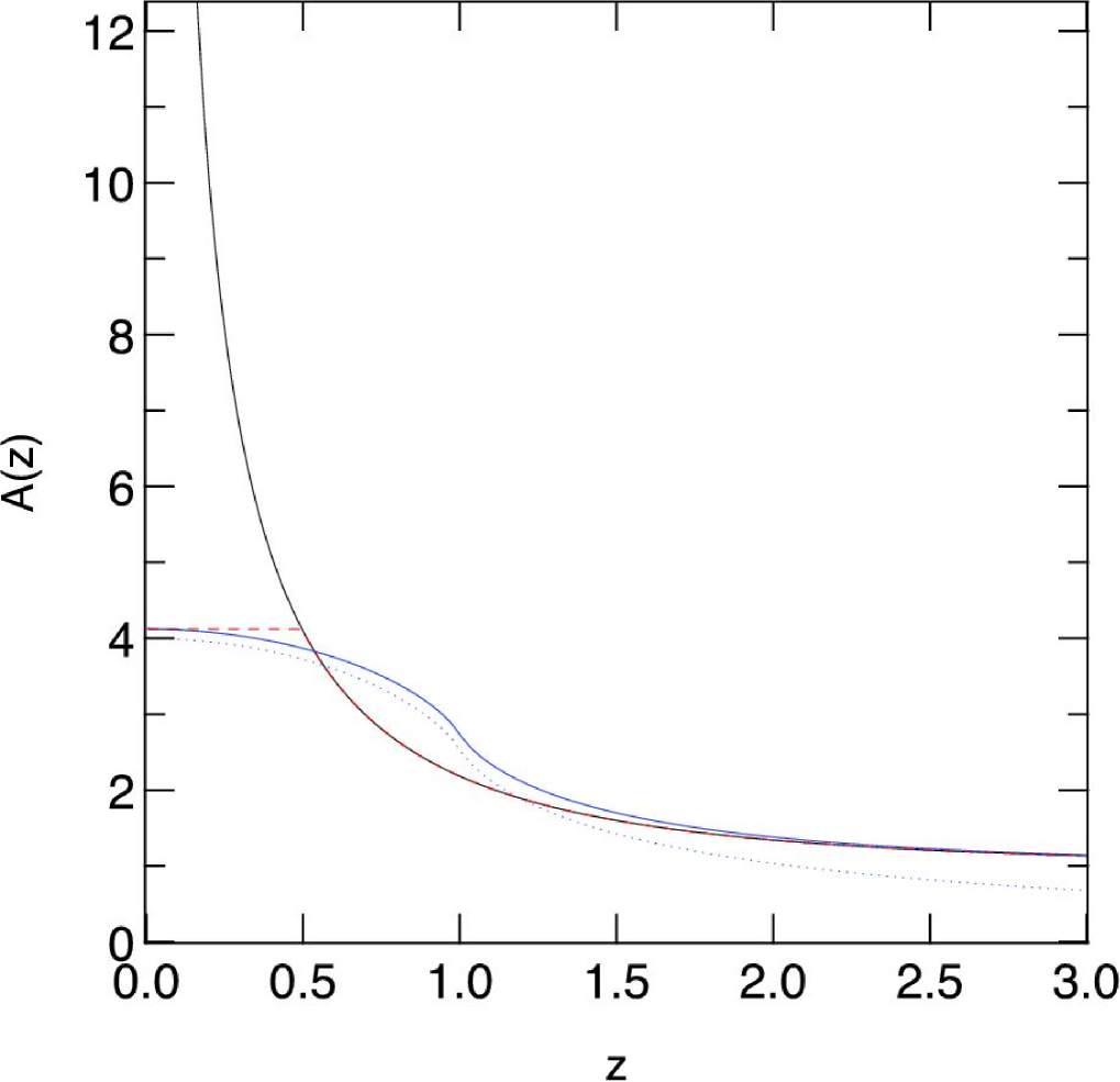
Figure 1.— Amplification $A(z)$ versus $z(t):=\left[r(t)/R_{\ast}\right]\left({D_{\mathrm{os}}}/{D_{\mathrm{ol}}}\right)$ plotted for $R_{\ast}/{D_{\mathrm{os}}}=0.5\left({R_{\mathrm{E}}}/{D_{\mathrm{ol}}}\right)$. Black curve: point-source approximation, see equation (2). Blue curve: finite source magnification ${A^{\ast}}(z)$ for a homogeneously radiating disk of size $R_{\ast}$, exact solution, see equation (12). Red dashed curve: simple approximation ${A^{\ast}}(z)$ for finite source effects according to equation (15). Blue dots: finite source size approximation in the high-magnification regime, introduced by (Gould, 1994b, eq. (2.5)).

For small source-lens distances with ${D_{\mathrm{ol}}}\approx{D_{\mathrm{os}}}$ (e.g., for bulge-bulge self-lensing) the above relation becomes

$${A_{0}^{\ast}}\approx\sqrt{1+1.5\times 10^{6}\,\frac{{M}}{{M}_{\odot}}\left(\frac{R_{\ast}}{R_{\odot}}\right)^{-2}\frac{{D_{\mathrm{os}}}-{D_{\mathrm{ol}}}}{1\,\mathrm{kpc}}}.$$

For a source radius of supergiants of $R_{\ast}\approx 200R_{\odot}$ a source-lens distance of $1\,\mathrm{kpc}$, and a lens with ${M}=1{M}_{\odot}$ finite source effects already arise above a magnification of ${A_{0}^{\ast}}\approx 6.2$. For smaller masses ${M}=0.1{M}_{\odot}$ finite source effects become important even at a low magnification ${A_{0}^{\ast}}\approx 2$. Although typical source radii are smaller, this example shows that finite-source effects cannot be neglected. We will show in § 6.3 and Table 2 that indeed a large fraction of the M31 bulge-bulge lensing events will show finite source effects.

Figure 1 shows that for $u<{u_{0}^{\ast}}$ (or $z{\,\stackrel{{\scriptstyle\scriptstyle<}}{{\scriptstyle\sim}}\,}\frac{1}{2}$) with

$${u_{0}^{\ast}}:=u({A_{0}^{\ast}})=\,\left\{2\left[1+\left(\frac{R_{\ast}\,{D_{\mathrm{ol}}}}{2\,{R_{\mathrm{E}}}\,{D_{\mathrm{os}}}}\right)^{2}\right]^{1/2}-2\right\}^{1/2}\stackrel{{\scriptstyle{A_{0}^{\ast}}\gg 1}}{{\approx}}\frac{R_{\ast}{D_{\mathrm{ol}}}}{2{R_{\mathrm{E}}}{D_{\mathrm{os}}}},$$ (14)

the amplification is no longer directly connected to the source-lens separation (Gould, 1995), but all $u<{u_{0}^{\ast}}$ have nearly the same amplification equal to the point-source approximation $A(u)$ at ${u_{0}^{\ast}}$. Therefore we generalize equation (2) to approximately account for finite-source effects

$${A^{\ast}}(u)\approx\left\{\begin{array}[]{ll}\sqrt{1+\left(\frac{2\,{R_{\mathrm{E}}}\,{D_{\mathrm{os}}}}{R_{\ast}\,{D_{\mathrm{ol}}}}\right)^{2}},&u<{u_{0}^{\ast}}\\ \frac{u^{2}+2}{u\sqrt{u^{2}+4}},&u\geq{u_{0}^{\ast}}.\\ \end{array}\right.$$ (15)

For light curves with finite source signatures ($u_{0}<{u_{0}^{\ast}}$) at an impact parameter

$$u{\left(1+({A_{0}^{\ast}}-1)/2\right)}\stackrel{{\scriptstyle{A_{0}^{\ast}}\gg 1}}{{\approx}}(R_{\ast}\;{D_{\mathrm{ol}}})/({R_{\mathrm{E}}}\;{D_{\mathrm{os}}})$$

(or $z\approx 1$) the amplification of our approximation is half of the maximum and can be used to define the ${t^{\ast}_{\mathrm{FWHM}}}$:

$$\begin{array}[]{rcl}{t^{\ast}_{\mathrm{FWHM}}}&:=&{t_{\mathrm{E}}}{\Upsilon^{\ast}}:=\frac{2{R_{\mathrm{E}}}}{{v_{\mathrm{t}}}}\sqrt{u{\left(\frac{{A_{0}^{\ast}}+1}{2}\right)}^{2}-{u_{0}}^{2}}\stackrel{{\scriptstyle{A_{0}^{\ast}}\gg 1}}{{\approx}}2{t_{\mathrm{E}}}\;\sqrt{\left(\frac{2}{{A_{0}^{\ast}}}\right)^{2}-{u_{0}}^{2}}\\ &\approx&2{t_{\mathrm{E}}}\;\sqrt{\left(\frac{R_{\ast}\;{D_{\mathrm{ol}}}}{{R_{\mathrm{E}}}\;{D_{\mathrm{os}}}}\right)^{2}-{u_{0}}^{2}}\approx{t_{\mathrm{FWHM}}}\;\frac{1}{\sqrt{3}}\sqrt{\left(\frac{R_{\ast}\;{D_{\mathrm{ol}}}}{b\;{D_{\mathrm{os}}}}\right)^{2}-1}\geq{t_{\mathrm{FWHM}}}\quad{u_{0}}<{u_{0}^{\ast}}.\end{array}$$ (16)

with

$${\Upsilon^{\ast}}({u_{0}},R_{\ast},{D_{\mathrm{ol}}},{D_{\mathrm{os}}},{M}):=2\sqrt{u{\left(\frac{{A_{0}^{\ast}}+1}{2}\right)}^{2}-{u_{0}}^{2}}=2\sqrt{\frac{2({A_{0}^{\ast}}+1)}{\sqrt{({A_{0}^{\ast}}-1)({A_{0}^{\ast}}+3)}}-2-{u_{0}}^{2}}.$$

In equation (16) the FWHM timescales for light curves that show finite source signatures are related to the values ${t_{\mathrm{FWHM}}}$ for the point-source approximation using equations (9) and (10). This demonstrates that the source does affect the timescale of an event severely: a source with an impact parameter of one-tenth the projected source radius will have an event timescale almost 6 times as long as that in the point-source approximation.

The shortest and longest FWHM timescales for an event with finite source signature (${u_{0}}\leq{u_{0}^{\ast}}$) are equal (insert ${u_{0}}={u_{0}^{\ast}}$ and ${u_{0}}=0$ into eq. [16]),

$$\begin{array}[]{l}{t^{\ast}_{\mathrm{FWHM,min}}}={t_{\mathrm{E}}}\Upsilon({A_{0}^{\ast}})\stackrel{{\scriptstyle{A_{0}^{\ast}}\gg 1}}{{\approx}}\sqrt{3}\;\frac{R_{\ast}\,{D_{\mathrm{ol}}}}{{v_{\mathrm{t}}}\;{D_{\mathrm{os}}}},\\ {t^{\ast}_{\mathrm{FWHM,max}}}=2{t_{\mathrm{E}}}\,u{\left(\frac{{A_{0}^{\ast}}+1}{2}\right)}\stackrel{{\scriptstyle{A_{0}^{\ast}}\gg 1}}{{\approx}}2\;\frac{R_{\ast}\,{D_{\mathrm{ol}}}}{{v_{\mathrm{t}}}\;{D_{\mathrm{os}}}}.\end{array}$$ (17)

For a given transversal velocity the minimum timescale becomes the larger, the larger the source sizes are.

The largest flux excess of a lensed, extended star becomes

$${\Delta_{F,\mathrm{max}}}=F_{0}({A_{0}^{\ast}}-1)=F_{0}\left[\sqrt{1+\frac{16G{M}\,{D_{\mathrm{os}}}({D_{\mathrm{os}}}-{D_{\mathrm{ol}}})}{c^{2}\,R_{\ast}^{2}\,{D_{\mathrm{ol}}}}}-1\right]\stackrel{{\scriptstyle{A_{0}^{\ast}}\gg 1}}{{\approx}}\frac{4\sqrt{G}}{c}\,\sqrt{\frac{{D_{\mathrm{os}}}({D_{\mathrm{os}}}-{D_{\mathrm{ol}}})}{{D_{\mathrm{ol}}}}}\;{\sqrt{{M}}}\;\frac{F_{0}}{R_{\ast}},$$ (18)

irrespective of whether the light curve shows finite source signatures.

2.2. Extracting Observables from Light Curves

2.2.1 Measuring ${\Delta_{F}}$ and ${t_{\mathrm{FWHM}}}$

In this section we present three methods for measuring the excess flux ${\Delta_{F}}$ at maximum and the FWHM time ${t_{\mathrm{FWHM}}}$. One can see in equations (9) and (16) that ${t_{\mathrm{E}}}$ and $u_{0}$ (or $A_{0}$) enter the value of ${t_{\mathrm{FWHM}}}$ as a product, giving rise to the “Einstein time magnification” degeneracy, which may lead to poor error estimates for ${t_{\mathrm{E}}}$ (and $u_{0}$) even for well-determined values of ${t_{\mathrm{FWHM}}}$ and ${\Delta_{F}}$.

Accounting for this degeneracy, Gould (1996b) approximated the Paczynski light curve with one fewer parameter for the special case of high amplification:

$$\Delta_{F}^{\mathrm{Gould}}(t)\approx{F_{\mathrm{eff}}}\left[\frac{(t-t_{0})^{2}}{{t_{\mathrm{eff}}}^{2}}+1\right]^{-1/2}.$$ (19)

The three free parameters are ${F_{\mathrm{eff}}}:=\frac{{F_{0}}}{{u_{0}}}$, ${t_{\mathrm{eff}}}:={u_{0}}\,{t_{\mathrm{E}}}$, and $t_{0}$. This approximation has turned out to be a very useful filter for detecting lensing events; however, it fails to describe light curves when the magnification is not very large. We suggest using

$${\Delta_{F}}(t)\approx{\Delta_{F}}\left[\frac{12(t-t_{0})^{2}}{{t_{\mathrm{FWHM}}}^{2}}+1\right]^{-1/2}$$ (20)

instead. This approximation provides a good description also for lower magnifications. The three free parameters of this approximation are the time of maximum $t_{0}$, the excess flux ${\Delta_{F}}$, and the FWHM timescale ${t_{\mathrm{FWHM}}}$.

Figure 2 shows that equation (20) better approximates the Paczynski light curve than the Gould approximation in the core and in the inner part of the wings, and also provides the correct value for ${t_{\mathrm{FWHM}}}$ and ${\Delta_{F}}$.

There are two situations that can require a fourth, additive, free parameter in the light curve fit. The first one is the transition regime from pixel-lensing to microlensing (i.e., where the errors are small enough to sample the wings of the light curve). We suggest using

$${\Delta_{F}}(t)\approx{F_{\mathrm{eff}}}\left[\frac{(t-t_{0})^{2}}{{t_{\mathrm{eff}}}^{2}}+1\right]^{-1/2}-{F_{0}},$$ (21)

which provides an excellent fit to the Paczynski light curve (see Fig. 2, green curve).

The second situation is the following: imagine that the photon noise of the background becoming larger and finally exceeding the unlensed flux of the star ${F_{0}}$. Then the star cannot be resolved anymore and the rms error of the baseline of the light curve becomes proportional $N_{\mathrm{data\ points}}^{-1/2}\,\sigma$. The (minimum) systematic error is given by the fact that the subtracted reference image (with error $\sigma_{\mathrm{ref}}$) is a sum of (high-quality) images, potentially including some of the amplified phases of the sources. This implies that there are fundamental limits to the accuracy of the baseline, and we thus require an additive parameter to account for that. The approximation of any pixel-lensing light curve then becomes

$${\Delta_{F}}(t)\approx{F_{\mathrm{eff}}}\left[\frac{(t-t_{0})^{2}}{{t_{\mathrm{eff}}}^{2}}+1\right]^{-1/2}+C.$$ (22)

In fact, numerical simulations showed that much more accurate values are derived for ${F_{\mathrm{eff}}}$ and ${t_{\mathrm{eff}}}$ if this additional constant $C$ is allowed for.

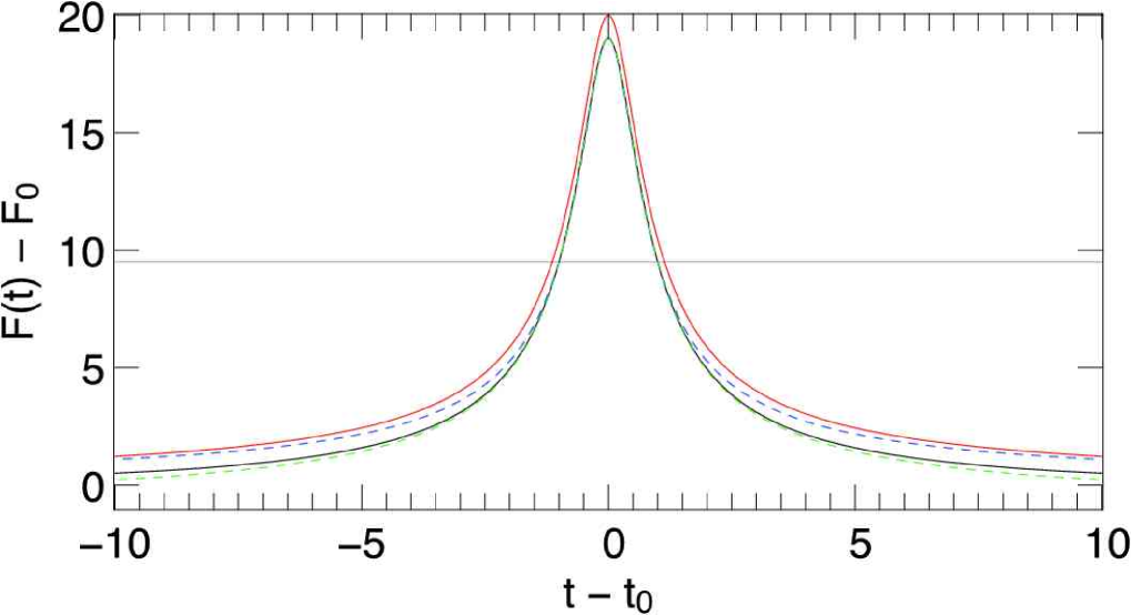
Figure 2.— Different light curve approximations using the following parameters: ${t_{\mathrm{FWHM}}}=2$, ${A_{0}}=20$, $F_{0}=1$, ${u_{0}}=0.05005$, and ${t_{\mathrm{E}}}=12.28$. Black curve: Paczynski (eqs. [1] and [2]). Red curve: Gould (eq. [19]). Blue dashed curve: Eq. [20]. Green dashed curve: Gould fit with additional free constant (eq. [21]). Gray line: ${\Delta_{F}}/2$ marks the flux level where ${t_{\mathrm{FWHM}}}$ is defined for the Paczynski curve.

2.2.2 Constraining ${F_{0}}$

In this section we address the important question, how to extract the source flux ${F_{0}}$ from a lensing light curve. There are four potential ways to constrain the flux of the lensed star:

1. The lensed star is resolved and isolated, and therefore a bias in the flux measurement (by crowding) can be excluded (assuming no systematic effects in the baseline). One would of course call such an event a classical microlensing event. A microlensing fit (using $\chi^{2}$ analysis methods) to the light curve then directly provides ${F_{0}}$ and its probability distribution, ideally given by an Gaussian error $\sigma_{F_{0}}$. In this case the flux measurement error is directly correlated to $Q$, the signal-to-noise ratio at maximum magnification.

2. The flux ${F_{0}}$ is obtained through the information that is in the shape of the wings of the difference light curve ${F_{0}}(A(t)-1)+C\equiv{F_{0}}A(t)+B$. The $\chi^{2}$ analysis leads to a probability distribution for ${F_{0}}$. This flux estimate method is used if no alternative unbiased flux measurement is available, i.e., cases in which the source star is resolved but blended (see (Alard, 1999) for applications in the microlensing regime), and cases in which the source star is not resolved (usually called a pixel-lensing event). Note that other methods using the shape of the wings (Baltz & Silk, 2000) provide similar results.

3. The flux ${F_{0}}$ is obtained from an additional, direct measurement, e.g., low-noise, high spatial resolution photometry from space.

4. The flux ${F_{0}}$ is constrained by theory through plausible distribution functions, e.g., the luminosity function $\Phi$, the color-magnitude relation of stars, and the distance distribution of stars, which together yield the source flux distribution function (see § 8.3). Another constraining example is an upper source flux limit that can be obtained from the fact that the source star is not resolved in the absence of lensing.

Since the physical processes are the same in pixel-lensing and microlensing, microlensing is a special case of pixel-lensing, where the source flux probability distribution is much more narrow than the stellar luminosity function, i.e., the distribution function used in the pixel-lensing regime. The methods only differ in how to analyze a light curve and how to derive the probability distribution for the source flux.

2.2.3 Evaluating ${t_{\mathrm{E}}}$

In this section we use the distribution of ${F_{0}}$ (from measurement or theory; see previous section) to estimate the probability distribution for a value of ${t_{\mathrm{E}}}$. Note that transforming the distribution of ${F_{0}}$ to a distribution of ${t_{\mathrm{E}}}$ can lead to a different value compared to a ${t_{\mathrm{E}}}$ obtained directly from the best estimate for ${F_{0}}$.

As the fitting process in the light curve analysis yields the non degenerate observables ${t_{\mathrm{FWHM}}}$ and ${\Delta_{F}}$, we can combine their (Gaussian) measurement errors with the probability distribution for the source flux ${F_{0}}$ and obtain the probablity distribution for ${t_{\mathrm{E}}}$:

$$\begin{array}[]{ll}{p_{{t_{\mathrm{E}}}}}({t_{\mathrm{E}}})&=\int\int\int\,p_{t_{\mathrm{FWHM}}}({t_{\mathrm{FWHM}}})\,p_{\Delta_{F}}({\Delta_{F}})\,p_{F_{0}}({F_{0}}))\,\delta{\left({t_{\mathrm{E}}}-\frac{{t_{\mathrm{FWHM}}}}{\Upsilon}\right)}\,d{t_{\mathrm{FWHM}}}\,d{\Delta_{F}}\,d{F_{0}}\\ &=\int\int\int\,p_{t_{\mathrm{FWHM}}}({t_{\mathrm{FWHM}}})\,p_{\Delta_{F}}({\Delta_{F}})\,p_{F_{0}}({F_{0}})\,\frac{\delta{\left({t_{\mathrm{FWHM}}}-{t_{\mathrm{E}}}\Upsilon\right)}}{\left|\Upsilon^{-1}\right|}\,d{t_{\mathrm{FWHM}}}\,d{\Delta_{F}}\,d{F_{0}}\\ &=\int\int\,p_{t_{\mathrm{FWHM}}}({t_{\mathrm{E}}}\Upsilon)\,p_{\Delta_{F}}({\Delta_{F}})\,p_{F_{0}}({F_{0}})\Upsilon{\left(\frac{{\Delta_{F}}}{{F_{0}}}+1\right)}\,d{\Delta_{F}}\,d{F_{0}}.\end{array}$$ (23)

This also allows to include non-Gaussian distributions for the source flux.

By transforming the measurements of ${\Delta_{F}}$ and ${t_{\mathrm{FWHM}}}$ together with a probability distribution of ${F_{0}}$, we derive a general formalism that is applicable to all microlensing and pixel-lensing problems. In § 8 we further develop this idea using plausible distribution functions as physical constraints, which narrows the width of the distribution of the lens mass ${M}$ (connected to ${t_{\mathrm{E}}}$).

3. Distribution Function for Lens Parameters

For a source of fixed intrinsic flux ${F_{0}}$, position $\vec{r}_{s}=(x,y,{D_{\mathrm{os}}})$ and velocity vector ${\vec{v}_{s}}=({v_{s,x}},{v_{s,y}},{v_{s,z}})$, the number and characteristics of lensing events are determined by the probability function $p(\vec{r}_{l},{\vec{v}_{l}},{M})$ for a lens with mass ${M}$ and velocity ${\vec{v}_{l}}$ being at position $\vec{r}_{l}$. For the change of magnification of the background source, only the transversal velocity components of source and lens are relevant (we assume velocities to be constant). For parallax microlensing events (Gould, 1994a, b) the nonuniform velocity of the observer changes the observed light curves, since the observer’s reference frame is not fixed. However, this effect is unimportant for extragalactic microlensing events.

Therefore, in addition to ${M}$ and ${D_{\mathrm{ol}}}$ only the projected relative transversal positions $r:=r_{\mathrm{t},l}-\frac{{D_{\mathrm{ol}}}}{{D_{\mathrm{os}}}}r_{\mathrm{t},s}$ and velocities ${v_{\mathrm{t}}}:=v_{\mathrm{t},l}-\frac{{D_{\mathrm{ol}}}}{{D_{\mathrm{os}}}}v_{\mathrm{t},s}$ and the angle $\phi$ enclosed by relative position and velocity vector enter the lensing properties. The distributions in $r$ and $\phi$ can be reduced to the distribution of one parameter, the impact parameter $b$ of the lens-source trajectory. This is obvious, since in a symmetric potential the trajectory of a particle is fully described by its minimum distance.

So, the relevant lens parameters are ${D_{\mathrm{ol}}}$, ${v_{\mathrm{t}}}$, ${M}$, and $b$. We introduce the lens density and the distributions of ${D_{\mathrm{ol}}}$, ${v_{\mathrm{t}}}$, and ${M}$ in the next two subsections and then come up with a new lensing event definition in § 3.3. For those lenses that satisfy the event definition, i.e., those which cause events, we will then derive the distribution of the impact parameters $dN/db$. We will show that our event definition gives the familiar relation for the event rate but is more easy to implement in numerical simulations.

3.1. Distance and Mass Distribution

The probability distributions for a lens with mass ${M}$ being at distance ${D_{\mathrm{ol}}}$ are given by

$$p_{D_{\mathrm{ol}}}=\rho({D_{\mathrm{ol}}})\,\left[\int\limits_{0}^{D_{\mathrm{os}}}{\rho({D_{\mathrm{ol}}})\,d{D_{\mathrm{ol}}}}\right]^{-1},$$ (24)

$$p_{M}=\xi({M})\,\left[\int\limits_{0}^{\infty}{\xi({M})\,d{M}}\right]^{-1},$$ (25)

where $\rho({D_{\mathrm{ol}}})$ is the lens mass density and $\xi({M})$ is the lens mass function (which itself is normalized to $\int\xi({M}){M}d{M}=1$; see Binney & Tremaine (1987, p. 747)). The number density per lens mass interval finally is defined by

$$n({D_{\mathrm{ol}}},{M}):=\rho({D_{\mathrm{ol}}})\,\xi({M}),$$ (26)

where $n({D_{\mathrm{ol}}},{M})$ has units of $\mathrm{length}^{-3}\,\mathrm{mass}^{-1}$.

3.2. Velocity Distribution for Lenses

We assume that the velocity distribution of the lenses around their mean streaming velocity is Gaussian:

$$p({v_{l,i}}) = C_{l}\,e^{-\frac{{v_{l}}_{i}^{2}}{2{\sigma_{\mathrm{l}}}^{2}}},\quad i=x,y,z,\quad C_{l}=\frac{1}{\sqrt{2\pi}\,{\sigma_{\mathrm{l}}}}.$$

where ${\sigma_{\mathrm{l}}}$ is the dispersion and depends on the position $(x,y,z)$. We furthermore assume that the combined transverse motion of observer and source relative to the mean transverse streaming velocity of the lenses is known and occurs in the $x$-direction with amplitude $v_{0}(x,y,z)$ as projected onto the lens plane. This means that the velocity $v_{s}$ of the source turns into a projected velocity $v_{p}={D_{\mathrm{ol}}}/{D_{\mathrm{os}}}\,v_{s}$ (lensing timescales are determined by relative proper motions not absolute motions of lens and source).

We now define the relative projected velocity ${v_{ls,x}}:={v_{l,x}}+v_{0}$ (analogously ${v_{ls,y}}:={v_{l,y}}+0$) and obtain the transverse lens-source velocity distribution as

$$\begin{array}[]{rcl}{p_{v_{\mathrm{t}}}}({v_{\mathrm{t}}},v_{0})&=&\frac{1}{2\pi{\sigma_{\mathrm{l}}}^{2}}\int\limits_{-\infty}^{+\infty}\int\limits_{-\infty}^{+\infty}\delta{\left({v_{\mathrm{t}}}-\sqrt{{v_{ls,x}}^{2}+{v_{ls,y}}^{2}}\right)}\,\exp\left(-\frac{({v_{ls,x}}-v_{0})^{2}}{2{\sigma_{\mathrm{l}}}^{2}}\right)\,\exp\left(-\frac{{v_{ls,y}}^{2}}{2{\sigma_{\mathrm{l}}}^{2}}\right)\,d{v_{ls,y}}\,d{v_{ls,x}}\\ &=&\frac{1}{2\pi{\sigma_{\mathrm{l}}}^{2}}\int\limits_{-{v_{\mathrm{t}}}}^{{v_{\mathrm{t}}}}\int\limits_{-\infty}^{+\infty}\frac{\delta{\left({v_{ls,y}}-\sqrt{{v_{\mathrm{t}}}^{2}-{v_{ls,x}}^{2}}\right)}+\delta{\left({v_{ls,y}}+\sqrt{{v_{\mathrm{t}}}^{2}-{v_{ls,x}}^{2}}\right)}}{\left|{v_{ls,y}}/\sqrt{{v_{ls,x}}^{2}+{v_{ls,y}}^{2}}\right|}\,\exp\left(-\frac{({v_{ls,x}}-v_{0})^{2}}{2{\sigma_{\mathrm{l}}}^{2}}\right)\,\exp\left(-\frac{{v_{ls,y}}^{2}}{2{\sigma_{\mathrm{l}}}^{2}}\right)\,d{v_{ls,y}}\,d{v_{ls,x}}\\ &=&\int\limits_{-{v_{\mathrm{t}}}}^{{v_{\mathrm{t}}}}\frac{1}{\pi{\sigma_{\mathrm{l}}}^{2}}{v_{\mathrm{t}}}\,\exp\left(-\frac{{v_{\mathrm{t}}}^{2}+v_{0}^{2}}{2{\sigma_{\mathrm{l}}}^{2}}\right)\,\frac{\exp\left(-\frac{-2v_{0}{v_{ls,x}}}{2{\sigma_{\mathrm{l}}}^{2}}\right)}{\sqrt{{v_{\mathrm{t}}}^{2}-{v_{ls,x}}^{2}}}\,d{v_{ls,x}}\\ &=&\frac{1}{{\sigma_{\mathrm{l}}}^{2}}\,{v_{\mathrm{t}}}\,\exp\left(-\frac{{v_{\mathrm{t}}}^{2}+v_{0}^{2}}{2{\sigma_{\mathrm{l}}}^{2}}\right)I_{0}\left(\frac{v_{0}{v_{\mathrm{t}}}}{{\sigma_{\mathrm{l}}}^{2}}\right).\end{array}$$ (27)

Here the Bessel function $I_{0}$ stretches the distribution depending on $v_{0}$.

3.3. Impact Parameter Distribution for Events

In Paczyński (1986) definition for lensing events (hereafter called standard definition) lens-source configurations become lensing events if the magnification of a source rises above a given threshold within the survey time interval $\Delta t$. This means that for each lens mass one can define a “microlensing-tube” along the line-of-sight to the source, which separates the high-magnification region from the low-magnification region, and a lens causes an event if it enters the tube.

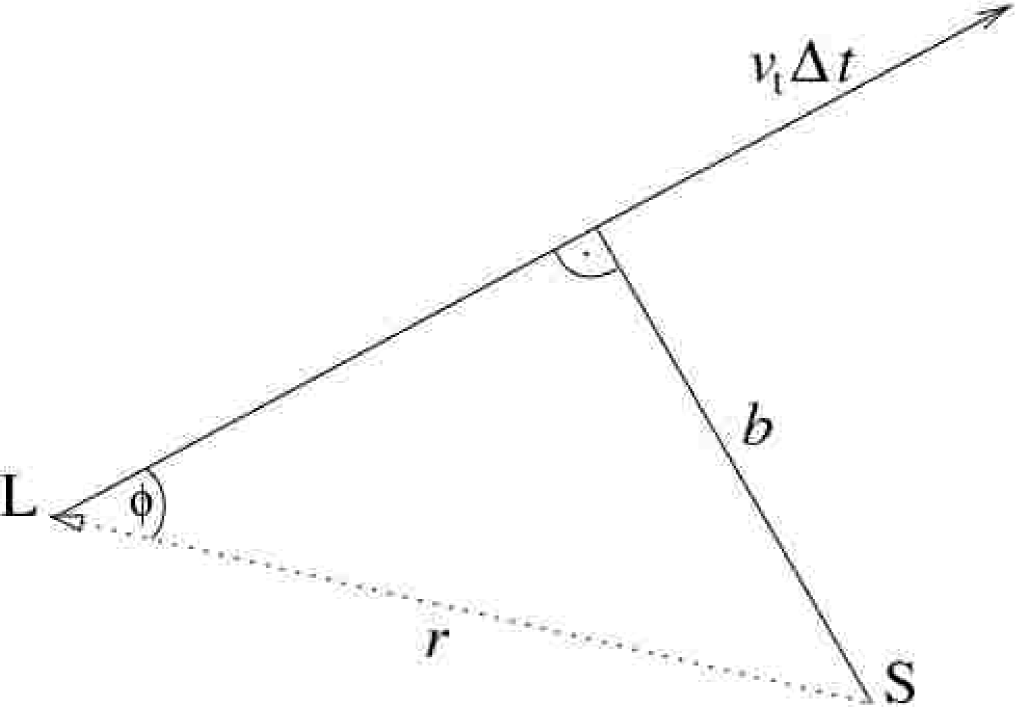
Figure 3.— For a projected lens-source separation $r$ and an angle $\phi$ between the projected distance vector and the projected relative velocity vector the impact parameter of the source-lens configuration is $b=r\sin(\phi)$. The lens approaches the source only for angles between $-\pi/2$ and $\pi/2$.

We use (for the motivation, see § A) an alternative event definition: a lens-source configuration becomes an event, if the lensing light curve reaches the maximum within the survey time $\Delta t$. This definition does not specify any specific magnification threshold at the time of maximum magnification because this magnification threshold will in reality depend on the observational setup and the brightness of the source. We show that the impact parameter distribution for the maximum light curve event definition agrees with the standard definition, if the same magnification threshold is used.

For simplicity we consider lenses with one mass, distance, and velocity, for the moment only. The lenses are homogeneously distributed points (in two dimensions) with density $n$ and velocities of ${v_{\mathrm{t}}}$ (the velocities can have arbitrary directions, but the angular distribution of the velocities must be the same for all the points). The number of lenses per radius interval around the line-of-sight to the source is

$$\frac{dN}{dr}(r)=n\,2\pi r.$$ (28)

If $r$ is the source-lens distance at the beginning of the survey and $\phi$ is the angle that the lens’s velocity vector encloses with the lens-source vector at that time, then the configuration will become an event with impact parameter $b$ if $b\leq r\leq\sqrt{b^{2}+({v_{\mathrm{t}}}\Delta t)^{2}}$ and $b=r|\sin(\phi)|$ with $\phi\in[-\pi/2,\pi/2]$ holds (see Figure 3 and § A). Therefore, $\frac{dN}{db}$ can be derived from the spatial distribution of the lenses relative to the source, $\frac{dN}{dr}$, and the distribution of the angles between velocity vector and distance to the source. For the special case in which all lenses have isotropic velocities of ${v_{\mathrm{t}}}$, the probability for the angle between radius vector and velocity vector is independent of the location of the lens and equals

$${p_{\phi}}(\phi):=\frac{1}{2\pi},\quad 0\leq\phi\leq 2\pi,$$ (29)

and

$$\begin{array}[]{ll}\frac{dN}{db}(b)&=\int\limits_{b}^{\sqrt{({v_{\mathrm{t}}}\Delta t)^{2}+b^{2}}}\,2\int\limits_{0}^{\pi/2}\,\frac{dN}{dr}\,\frac{1}{2\pi}\,\delta(b-r\sin\phi)\,d\phi\,dr=n\,\int\limits_{b}^{\sqrt{({v_{\mathrm{t}}}\Delta t)^{2}+b^{2}}}\,2\int\limits_{0}^{\pi/2}r\,\frac{\delta{\left(\phi-\arcsin\frac{b}{r}\right)}}{\sqrt{r^{2}-(r\sin\phi)^{2}}}\,d\phi\,dr\\ &=n\,\int\limits_{b}^{\sqrt{({v_{\mathrm{t}}}\Delta t)^{2}+b^{2}}}\,\frac{2r}{\sqrt{r^{2}-b^{2}}}\,dr=2n\,{v_{\mathrm{t}}}\Delta t.\end{array}$$ (30)

In this equation, the radial integration limits correspond to the minimum and maximum source-lens separation for an event with impact parameter $b$ within $\Delta t$, and the $\delta$-function then allows only for those trajectories through $r$ that have the correct angle $\phi$ for the impact parameter $b=r\sin(\phi)$ of interest. The factor of 2 accounts for integrating from $0$ to $\pi/2$ instead of $-\pi/2$ to $\pi/2$ in the angle. In the second line of this equation we have changed the variable in the $\delta$-function from $r\sin(\phi)$ to $\phi$ and then have carried out the angle integration and finally the r-integration. The quantity $\frac{dN}{db}$ has units of $\mathrm{length}^{-1}$.

Note that $\frac{dN}{db}$ is independent of $b$; i.e., the impact parameters of the events are uniformly distributed. Of course, in reality, an upper limit $b_{\rm max}$ will be present, depending on the source brightness, background light and the observing conditions. The integral $\int_{0}^{b_{\rm max}}\frac{dN}{db}db=2n\,{v_{\mathrm{t}}}\,\Delta t\times b_{\rm max}$ is dimensionless and equals (for the considered line-of-sight) the number of lenses that cause an event above a minimum magnification (corresponding to $b_{\rm max}$) within $\Delta t$.

Equation (30) can also be obtained from geometrical arguments: a circle with radius $b$ embedded into a two dimensional plane defines a cross section of $2b$ to streaming particles in that plane, independent of the streaming direction. Therefore, the number of particles passing through that aperture with diameter $2b$ in a time $\Delta t$ is $n{v_{\mathrm{t}}}\Delta t2b$. Hence, equation (30) also holds for a coherent particle stream, with any velocity direction. Therefore equation (30) is also valid for any probability distribution of the velocity angles.

The number of events per line-of-sight distance ${D_{\mathrm{ol}}}$, lens mass ${M}$, transversal velocity ${v_{\mathrm{t}}}$, and impact parameter $b$ follows from equation (30) by replacing $n$ with $n({D_{\mathrm{ol}}},{M},{v_{\mathrm{t}}})=n({D_{\mathrm{ol}}},{M})\,{p_{v_{\mathrm{t}}}}({v_{\mathrm{t}}},{D_{\mathrm{ol}}})$:

$$\frac{d^{4}N}{d{D_{\mathrm{ol}}}\,d{M}\,d{v_{\mathrm{t}}}\,db}=2\,n({D_{\mathrm{ol}}},{M})\,{p_{v_{\mathrm{t}}}}({v_{\mathrm{t}}},{D_{\mathrm{ol}}})\,{v_{\mathrm{t}}}\Delta t=2\,\rho({D_{\mathrm{ol}}})\,\xi({M})\,{p_{v_{\mathrm{t}}}}({v_{\mathrm{t}}},{D_{\mathrm{ol}}})\,{v_{\mathrm{t}}}{\Delta t}.$$ (31)

We now transfer the number $N$ of the events per line-of-sight to the event rate (per line-of-sight), $\Gamma:=\frac{N}{{\Delta t}}$, and write equation (31) as

$$\frac{d^{4}\Gamma}{d{D_{\mathrm{ol}}}\,d{M}\,d{v_{\mathrm{t}}}\,db}=2\,\rho({D_{\mathrm{ol}}})\,\xi({M})\,{p_{v_{\mathrm{t}}}}({v_{\mathrm{t}}},{D_{\mathrm{ol}}})\,{v_{\mathrm{t}}}.$$ (32)

With the relative impact parameter ${u_{0}}$ defined as ${u_{0}}=\frac{b}{{R_{\mathrm{E}}}({D_{\mathrm{ol}}},{M})}$ this distribution can be rewritten as

$$\frac{d^{4}\Gamma}{d{D_{\mathrm{ol}}}\,d{M}\,d{v_{\mathrm{t}}}\,d{u_{0}}}=2\,\rho({D_{\mathrm{ol}}})\,\xi({M})\,{p_{v_{\mathrm{t}}}}({v_{\mathrm{t}}},{D_{\mathrm{ol}}})\,{v_{\mathrm{t}}}\,{R_{\mathrm{E}}}({D_{\mathrm{ol}}},{M}),$$ (33)

which corresponds to the event rate for the standard definition (see de Rujula et al. (1991)).

4. The Source Distributions

In the case of pixel-lensing the parameters of the source cannot be determined. Therefore, we now introduce probability distributions for the source distance ${D_{\mathrm{os}}}$, velocity ${\vec{v}_{s}}$, unlensed flux ${F_{0}}$, color ${\mathcal{C}}$, and radius $R_{\ast}$ (for finite source effects).

4.1. The Transverse Lens-source Velocity Distribution

We again assume that the velocity distributions of lenses $l$ and sources $s$ are approximately isotropic around their mean respective streaming velocities (cf. equation (3.2)). The projected velocity dispersion of the source population we call ${\tilde{\sigma}_{\mathrm{s}}}={D_{\mathrm{ol}}}/{D_{\mathrm{os}}}\,{\sigma_{\mathrm{s}}}$. We define $\vec{v}_{0}=({v_{0,x}},{v_{0,y}})$ as the difference between the projected streaming velocities of the source and lens populations. Then, the transverse velocity differences in $x$ and $y$ between a lens and a source, each drawn from their respective distributions, are: ${v_{ls,x}}:={v_{l,x}}-{v_{s,x}}+{v_{0,x}}$ and ${v_{ls,y}}:={v_{l,y}}-{v_{s,y}}+{v_{0,y}}$.

Similar to equation (27), we obtain for the distribution of the transverse velocities

$${p_{v_{\mathrm{t}}}}({v_{\mathrm{t}}},v_{0})=\int\limits\delta\left({v_{\mathrm{t}}}-\sqrt{{v_{ls,x}}^{2}+{v_{ls,y}}^{2}}\right)p({v_{ls,x}})\,p({v_{ls,y}})\,d{v_{ls,x}}\,d{v_{ls,y}},$$ (34)

where $p({v_{ls,x}})$ [and $p({v_{ls,y}})$ analogously] is given by

$$\begin{array}[]{ll}p({v_{ls,x}})&=C_{l}C_{s}\int\limits_{-\infty}^{+\infty}\int\limits_{-\infty}^{+\infty}\exp\left(-\frac{{\tilde{\sigma}_{\mathrm{s}}}^{2}{v_{l,x}}^{2}+{\sigma_{\mathrm{l}}}^{2}{v_{s,x}}^{2}}{2{\sigma_{\mathrm{l}}}^{2}{\tilde{\sigma}_{\mathrm{s}}}^{2}}\right)\delta({v_{ls,x}}-({v_{l,x}}-{v_{s,x}}+{v_{0,x}}))\,d{v_{l,x}}\,d{v_{s,x}}\\ &=C_{l}C_{s}\int\limits_{-\infty}^{+\infty}\int\limits_{-\infty}^{+\infty}\exp\left(-\frac{{\tilde{\sigma}_{\mathrm{s}}}^{2}{v_{l,x}}^{2}+{\sigma_{\mathrm{l}}}^{2}{v_{s,x}}^{2}}{2{\sigma_{\mathrm{l}}}^{2}{\tilde{\sigma}_{\mathrm{s}}}^{2}}\right)\delta({v_{l,x}}-({v_{ls,x}}+{v_{s,x}}-{v_{0,x}}))\,d{v_{l,x}}\,d{v_{s,x}}\\ &=C_{l}C_{s}\int\limits_{-\infty}^{+\infty}\exp\left(-\frac{({v_{ls,x}}-{v_{0,x}})^{2}}{2({\sigma_{\mathrm{l}}}^{2}+{\tilde{\sigma}_{\mathrm{s}}}^{2})}\right)\sqrt{\frac{2\pi{\sigma_{\mathrm{l}}}^{2}{\tilde{\sigma}_{\mathrm{s}}}^{2}}{{\sigma_{\mathrm{l}}}^{2}+{\tilde{\sigma}_{\mathrm{s}}}^{2}}}\,d{v_{ls,x}}\\ &=\frac{1}{\sqrt{{\sigma_{\mathrm{l}}}^{2}+{\tilde{\sigma}_{\mathrm{s}}}^{2}}\,\sqrt{2\pi}}\,\exp\left(-\frac{({v_{ls,x}}-{v_{0,x}})^{2}}{2({\sigma_{\mathrm{l}}}^{2}+{\tilde{\sigma}_{\mathrm{s}}}^{2})}\right)\\ &=\frac{1}{{\sigma_{\mathrm{ls}}}\,\sqrt{2\pi}}\,\exp\left(-\frac{({v_{ls,x}}-{v_{0,x}})^{2}}{2{\sigma_{\mathrm{ls}}}^{2}}\right).\\ \end{array}$$ (35)

In the last step we have defined

$${\sigma_{\mathrm{ls}}}:=\sqrt{{\sigma_{\mathrm{l}}}^{2}+\left(\frac{{D_{\mathrm{ol}}}}{{D_{\mathrm{os}}}}\right)^{2}{\sigma_{\mathrm{s}}}^{2}},$$ (36)

which is the combined width of the velocity distribution of the lenses and that of the sources, projected onto the lens plane.

Finally, analogously to equation (27), we obtain

$${p_{v_{\mathrm{t}}}}({v_{\mathrm{t}}},v_{0})=\frac{1}{{\sigma_{\mathrm{ls}}}^{2}}\,{v_{\mathrm{t}}}\,\exp{\left(-\frac{{v_{\mathrm{t}}}^{2}+v_{0}^{2}}{2{\sigma_{\mathrm{ls}}}^{2}}\right)}\,I_{0}{\left(\frac{v_{0}\,{v_{\mathrm{t}}}}{{\sigma_{\mathrm{ls}}}^{2}}\right)},$$ (37)

with $v_{0}(x,y,{D_{\mathrm{ol}}},{D_{\mathrm{os}}})$, ${\sigma_{\mathrm{l}}}(x,y,{D_{\mathrm{ol}}})$, and ${\sigma_{\mathrm{s}}}(x,y,{D_{\mathrm{os}}})$.

4.2. The Luminosity Function

The luminosity function (LF) $\phi\left(\mathrm{flux}^{-1}\right)$ or $\Phi\left(\mathrm{mag}^{-1}\right)$ is usually defined as the number of stars per luminosity bin.

The mean, or so-called characteristic flux of a stellar population is

$$<{\mathcal{F}}>:=\frac{\int{\mathcal{F}}\,\phi({\mathcal{F}})\,d{\mathcal{F}}}{\int\phi({\mathcal{F}})\,d{\mathcal{F}}},$$ (38)

or, if one instead uses the luminosity function $\Phi$ in magnitudes,

$$<{\mathcal{F}}>:=\frac{\int{F_{\mathrm{Vega}}}10^{-0.4{\mathcal{M}}}\,\Phi({\mathcal{M}})\,d{\mathcal{M}}}{\int\Phi({\mathcal{M}})\,d{\mathcal{M}}},$$ (39)

where ${F_{\mathrm{Vega}}}$ is the flux of Vega.

We use a luminosity function normalized equal to 1,

$$\int\limits_{0}^{\infty}\tilde{\phi}({\mathcal{F}})\,d{\mathcal{F}}:=\int\limits_{-\infty}^{+\infty}\tilde{\Phi}({\mathcal{M}})\,d{\mathcal{M}}:=1,$$ (40)

as we obtain the amplitude of the LF from the matter density and the mass-to-light ratio of the matter components (bulge, disk) later on.

The luminosity functions in the literature are usually given for stars at a distance of 10 pc. The relations for the source flux ${F_{0}}$ at a distance ${D_{\mathrm{os}}}$ and its flux ${\mathcal{F}}$ at 10 pc, or its absolute magnitude ${\mathcal{M}}$ are given in the following two equations, allowing for extinction along the line-of-sight:

$${F_{0}}({\mathcal{F}},x,y,{D_{\mathrm{os}}}):={\mathcal{F}}\times\left(\frac{10\,\mathrm{pc}}{{D_{\mathrm{os}}}}\right)^{2}\,10^{-0.4\,\mathcal{A}(x,y,{D_{\mathrm{os}}})},$$ (41)

$$\begin{array}[]{l}{F_{0}}({\mathcal{M}},x,y,{D_{\mathrm{os}}}):={F_{\mathrm{Vega}}}10^{-0.4{\mathcal{M}}}\times\left(\frac{10\,\mathrm{pc}}{{D_{\mathrm{os}}}}\right)^{2}\,10^{-0.4\,\mathcal{A}(x,y,{D_{\mathrm{os}}})}.\end{array}$$ (42)

4.3. The Number Density of Sources

We characterize different source components (bulge and disk) by an index ${s}$ with corresponding indices in the density, luminosity, and mass-function of that component. $(M/L)_{s}$ is the mass-to-light ratio of that component in solar units.

The number density of sources is a function of the mass density, the mass-to-light ratio, and the characteristic flux of each component:

$$n_{s}(x,y,{D_{\mathrm{os}}}):=\frac{d^{3}{N_{s}}}{dx\,dy\,d{D_{\mathrm{os}}}}=\frac{\,\rho_{s}(x,y,{D_{\mathrm{os}}})}{{\left(\frac{M}{L}\right)}_{s}\,\frac{{M}_{\odot}}{{\mathcal{F}}_{\odot}}\,<{\mathcal{F}}>_{s}}.$$ (43)

Note that $(M/L)$ is the mass-to-light ratio of the total disk or bulge component, and has to include the mass in stellar remnants or in gas. Therefore, the value of $(M/L)$ is not necessarily equal to the stellar mass-to-light-ratio in the bulge and the disk.

The normalized probability distribution for sources $p_{s}({D_{\mathrm{os}}})$ at distance ${D_{\mathrm{os}}}$ is

$$p_{s}({D_{\mathrm{os}}}):=\frac{\rho_{s}({D_{\mathrm{os}}})}{\int\limits_{0}^{\infty}{\rho_{s}({D_{\mathrm{os}}})\,d{D_{\mathrm{os}}}}}.$$ (44)

4.4. Including the Color and Radius Information

To use the color information, ${\mathcal{C}}:={\mathcal{M}}-{\mathcal{M}}`$, we construct a normalized color-flux distribution ${p_{\mathrm{cmd}}}({\mathcal{M}},{\mathcal{C}})$ from the color-magnitude diagram of stars,

$$\int\int{p_{\mathrm{cmd}}}({\mathcal{M}},{\mathcal{C}})\,d{\mathcal{M}}\,d{\mathcal{C}}\stackrel{{\scriptstyle!}}{{=}}1,$$ (45)

which is related to the luminosity function as

$$\tilde{\Phi}({\mathcal{M}})=\int{p_{\mathrm{cmd}}}({\mathcal{M}},{\mathcal{C}})\,d{\mathcal{C}}.$$ (46)

The radius is related to the luminosity and color as $R_{\ast}({\mathcal{M}},{\mathcal{C}})$ (see § B.4).

5. Applications for the Microlensing Regime

In this section we derive the basic microlensing quantities and distributions using the four-dimensional event rate differential derived in § 3. We apply the equations to M31 using the M31 model in § B.

5.1. Optical Depth $\tau$

The optical depth $\tau$ is defined as the number of lenses that are closer than their own Einstein radius ${R_{\mathrm{E}}}$ to a line-of-sight. The optical depth $\tau$ is therefore the instantaneous probability of lensing taking place, given a line-of-sight and a density distribution of the lenses. For a given source star at distance ${D_{\mathrm{os}}}$, the optical depth equals the number of lenses within the microlensing tube defined by the Einstein radius ${R_{\mathrm{E}}}({M},{D_{\mathrm{ol}}},{D_{\mathrm{os}}})$ (eq. [4]) along the line-of-sight:

$$\begin{array}[]{ll}\tau({D_{\mathrm{os}}})&=\int\limits_{0}^{D_{\mathrm{os}}}\int\limits_{0}^{\infty}\int\limits_{0}^{\infty}\int\limits_{0}^{{R_{\mathrm{E}}}}n({D_{\mathrm{ol}}},{M},{v_{\mathrm{t}}})\times 2\pi r\,dr\,d{v_{\mathrm{t}}}\,d{M}\,d{D_{\mathrm{ol}}}\\ &=\int\limits_{0}^{D_{\mathrm{os}}}\int\limits_{0}^{\infty}\int\limits_{0}^{\infty}\rho({D_{\mathrm{ol}}})\,\xi({M})\,{p_{v_{\mathrm{t}}}}({v_{\mathrm{t}}},{D_{\mathrm{ol}}})\,\int\limits_{0}^{{R_{\mathrm{E}}}}2\pi r\,dr\,d{v_{\mathrm{t}}}\,d{M}\,d{D_{\mathrm{ol}}}\\ &=\int\limits_{0}^{D_{\mathrm{os}}}\int\limits_{0}^{\infty}\rho({D_{\mathrm{ol}}})\,\xi({M})\,\pi{R_{\mathrm{E}}}^{2}\,d{M}\,d{D_{\mathrm{ol}}}\\ &=\frac{4\pi G}{c^{2}}\int\limits_{0}^{D_{\mathrm{os}}}\rho({D_{\mathrm{ol}}})\,D({D_{\mathrm{ol}}})\,d{D_{\mathrm{ol}}},\end{array}$$ (47)

with $D({D_{\mathrm{ol}}}):={D_{\mathrm{ol}}}({D_{\mathrm{os}}}-{D_{\mathrm{ol}}})/{D_{\mathrm{os}}}$, equal to Paczyński (1986, eq. (9)). Equation (47) demonstrates that the optical depth depends on the mass density, but not on the mass function $\xi({M})$ of the lenses.

In the past, the optical depth along a line-of-sight to M31 was often calculated by setting ${D_{\mathrm{os}}}$ equal to the distance to the plane of the disk of M31 (Gyuk & Crotts, 2000; Baltz & Silk, 2000). This is like treating the sources for lensing as a two dimensional distribution. It yields fairly adequate results for the optical depth of disk stars but cannot be justified for the bulge stars in M31. We use the source distance probability distribution (equation (44) to obtain the line-of-sight distance–averaged optical depth:

$$<\tau>_{s}\;:=\int p_{s}({D_{\mathrm{os}}})\,\tau({D_{\mathrm{os}}})\,d{D_{\mathrm{os}}}.$$ (48)

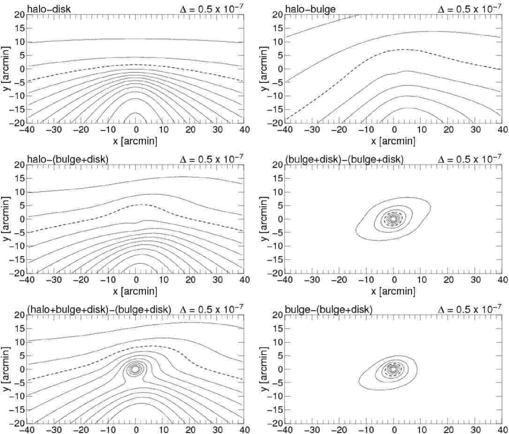
Figure 4.— Contours of the line-of-sight–averaged optical depth $\left<\tau\right>_{s}$ (eq. [48]). $x$ and $y$ are given in the intrinsic M31 coordinate system, which is centered on the nucleus of M31 and where the M31 disk major axis is orientated horizontally ($\mathrm{P}.\mathrm{A}.=38^{\circ}$). Halo lensing of disk sources (first row left, a), halo-bulge lensing (first row right,), halo-lensing of bulge & disk sources (second row left). The average optical depth for self-lensing of sources in M31 is shown in the second row on the right. In the third row, left panel, we show the resulting total optical depth with the contributions of all lenses. The third row, right panel, displays the optical depth due to bulge lenses. The optical depth caused by the MW (not shown), is nearly constant $\tau_{\mathrm{MW}}=0.78\times 10^{-6}$. To obtain the values of $<\tau>_{s}$ we used the model of the luminous and dark matter of M31 presented in § B. Here and in all following calculations a MACHO fraction in the dark halo of M31 of unity was assumed. The spacing between adjacent contours are shown as inserts in each diagram. The contour lines $<\tau>_{s}=2\times 10^{-6}$ are shown as dashed curve.

Figure 4 shows the average optical depth for the central part of M31 for lenses in the halo of M31 (“halo-lensing”), and for stellar lenses in the bulge and disk of M31 (“self-lensing”). The self-lensing optical depth is symmetric (with respect to the near and far side of M31) and dominates the optical depth in the central arcminute of M31. The halo-lensing optical depth is asymmetric and rises toward the far side of the M31 disk, since there are more halo lenses in front of the disk.

Figure 4 (first row, left) shows the halo-disk optical depth. The results do not depend so much on the three-dimensional structure of the disk but much more on the halo core radius assumed. We use $r_{\mathrm{c}}=2\,\mathrm{kpc}$ (see § B). Gyuk & Crotts (2000) used core radii of $r_{\mathrm{c}}=1\,\mathrm{kpc}$ and $r_{\mathrm{c}}=5\,\mathrm{kpc}$ for their Figures 1c and 1d, and our result is in between their results, as expected. Baltz & Silk (2000) have obtained qualitatively similar results using $r_{\mathrm{c}}=5\,\mathrm{kpc}$, but assuming an M31 distance of 725 kpc and a slightly less massive halo than we do. The optical depth caused by all M31 components is shown in Figure 4 (third row, left). The result of (Han, 1996, see his Fig. 1) using a halo core radius of $r_{\mathrm{c}}=6.5\,\mathrm{kpc}$ looks strikingly different. Comparison to Figure 4 (third row, left) demonstrates that the total optical depth is dominated by bulge lenses in the central part of M31. The last panel of this figure shows the optical depth for bulge-lensing toward M31 sources. The bulge-lensing optical depth had been obtained by (Gyuk & Crotts, 2000, see their Fig. 5), but the values that they obtained are up to a factor of 5 larger than ours (which probably is due to their different M31 model).

5.2. Single-star Event Rate

The optical depth is the probability of stars to be magnified above a threshold of 1.34 at any time. Observations, however, usually measure only a temporal change of magnification. Therefore, the event rate, which is the number of events per time interval, is the relevant quantity for observations. The event rate is the integral of equation (32) over lens masses, lens distances, relative velocities, and impact parameters $b$ smaller than a threshold ${u_{\mathrm{T}}}{R_{\mathrm{E}}}$:

$$\begin{array}[]{ll}\Gamma_{\mathrm{T}}({D_{\mathrm{os}}})&:=\int\limits_{0}^{\infty}\int\limits_{0}^{D_{\mathrm{os}}}\int\limits_{0}^{\infty}\,\int\limits_{0}^{{u_{\mathrm{T}}}{R_{\mathrm{E}}}}\frac{d^{4}\Gamma}{d{D_{\mathrm{ol}}}\,d{M}\,d{v_{\mathrm{t}}}\,db}\,db\,d{v_{\mathrm{t}}}\,d{M}\,d{D_{\mathrm{ol}}}\\ &=2{u_{\mathrm{T}}}\int\limits_{0}^{\infty}\,\xi({M})\int\limits_{0}^{D_{\mathrm{os}}}\,\rho({D_{\mathrm{ol}}})\,{R_{\mathrm{E}}}({D_{\mathrm{ol}}},{M})\int\limits_{0}^{\infty}{v_{\mathrm{t}}}\,{p_{v_{\mathrm{t}}}}({v_{\mathrm{t}}},{D_{\mathrm{ol}}})\,d{v_{\mathrm{t}}}\,d{D_{\mathrm{ol}}}\,d{M}\\ &=2{u_{\mathrm{T}}}\frac{\sqrt{4G}}{c}\int\limits_{0}^{D_{\mathrm{os}}}\rho({D_{\mathrm{ol}}})\,\sqrt{D({D_{\mathrm{ol}}})}\,\int\limits_{0}^{\infty}\sqrt{{M}}\,\xi({M})\int\limits_{0}^{\infty}{v_{\mathrm{t}}}\,{p_{v_{\mathrm{t}}}}({v_{\mathrm{t}}},{D_{\mathrm{ol}}})\,d{v_{\mathrm{t}}}\,d{D_{\mathrm{ol}}}\,d{M}\\ &=:{u_{\mathrm{T}}}\,\Gamma_{1}({D_{\mathrm{os}}}).\end{array}$$ (49)

This had been first evaluated [using a single mass instead of $\xi({M})$] by Griest (1991).

The impact parameter threshold ${u_{\mathrm{T}}}$ is equivalent to a magnification threshold ${A_{\mathrm{T}}}$. Therefore, the number of events with amplifications larger than ${A_{\mathrm{T}}}({u_{\mathrm{T}}})$ is proportional to the threshold parameter ${u_{\mathrm{T}}}$.

$\Gamma_{1}({D_{\mathrm{os}}})$ is the event rate along a chosen line-of-sight to a distance of ${D_{\mathrm{os}}}$. Analogously to the optical depth, we also define the line-of-sight distance–averaged single-star event rate

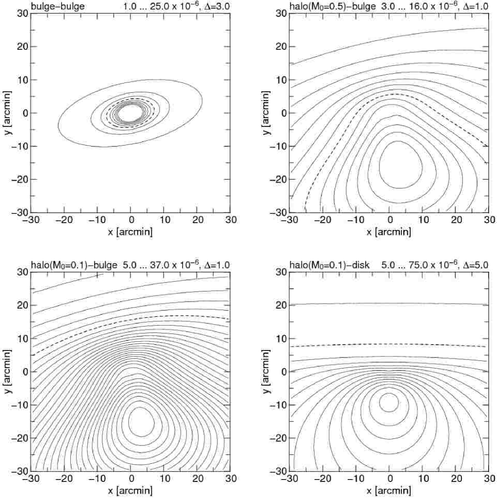
Figure 5.— Averaged event rate $<\Gamma_{1}>_{s}$ ($\mathrm{y}^{-1}$) toward M31 for bulge-bulge lensing first row, left), halo-bulge lensing with ${{M}_{0}}=0.5\,{{M}_{\odot}}$ (i.e., a mass function $\xi({M})=\delta({M}_{0}-0.5\,{{M}_{\odot}})/0.5\,{{M}_{\odot}}$) (first row, right), halo-bulge lensing with ${{M}_{0}}=0.1\,{{M}_{\odot}}$ (second row, left), and halo-disk lensing with ${{M}_{0}}=0.1\,{{M}_{\odot}}$ (second row, right). Contour levels and the spacing between adjacent contours are given on top of each diagram. The dashed line marks the $10^{-5}$ events $\,\mathrm{yr}^{-1}$ level. Whereas self-lensing is symmetric, halo lensing shows a clear asymmetry. The event rate shows a maximum at the far side of the M31 disk (negative $y$-values). These contours cannot be compared with an experiment since, first, one could certainly not identify all objects with a threshold of ${u_{\mathrm{T}}}=1$ or a magnification of $1.34$ and second, one has to convolve the single-star event rate with the density of sources. The proper event rate maps in the pixel-lensing regime can be seen in § 7.

$$<\Gamma_{1}>_{s}\;=\int p_{s}({D_{\mathrm{os}}})\,\Gamma_{1}({D_{\mathrm{os}}})\,d{D_{\mathrm{os}}}$$ (50)

toward M31.

We show these line-of-sight distance–averaged event rates for the halo of M31 and the stellar lenses in the bulge and disk of M31 (self-lensing) in Figure 5; the single-star halo-lensing event rate is evidently asymmetric, whereas the single-star self-lensing event rate is symmetric. The levels of the event rates (for each line-of-sight) are of the order $\sim 10^{-5}$ events $\,\mathrm{yr}^{-1}$ (dashed), which implies that at least a few times $10^{4}$ source stars are needed to identify one lensing event (even if all lensing events below the threshold ${u_{\mathrm{T}}}=1$ could be observed). It can also be seen in Figure 5 that only in the innermost part ($r\leq 5\arcmin$) the self-lensing event rate exceeds the halo-lensing event rate (for a 100% MACHO halo). As mentioned earlier, the optical depth does not depend on the lens-mass distribution (for the same matter density) because the decrease of number of lenses with lens-mass is balanced by the increased area of the Einstein disks around them. However, the events take longer, since larger Einstein radii have to be crossed. For the same optical depth, this then must imply a decrease in event rate: $\Gamma\sim{M}_{0}^{-1/2}$, setting $\xi({M})=\delta({M}-{M}_{0})/{M}_{0}$ in equation (49). The decrease of the event rate with increasing mass of the lenses can be seen in Figure 5 (first row, right panel) and Figure 5 (second row, left panel).

The relations above give the event rate per line-of-sight or per star. To compare this with measurements of the lensing rate for resolved stars, one has to account for the source density.

5.3. Distribution for the Einstein Timescale

Not only the number of lensing events per time and their spatial distribution but also their duration (Einstein time) is a key observable in microlensing surveys. The distribution of the Einstein timescales of the events is

$$\begin{array}[]{ll}\frac{d^{2}\Gamma}{d{t_{\mathrm{E}}}\,d{u_{0}}}&=\int\limits_{0}^{\infty}\int\limits_{0}^{D_{\mathrm{os}}}\int\limits_{0}^{\infty}\frac{d^{4}\Gamma}{d{D_{\mathrm{ol}}}\,d{M}\,d{v_{\mathrm{t}}}\,d{u_{0}}}\,\delta{\left({t_{\mathrm{E}}}-\frac{{R_{\mathrm{E}}}}{{v_{\mathrm{t}}}}\right)}\,d{v_{\mathrm{t}}}\,d{D_{\mathrm{ol}}}\,d{M}\\ &=\int\limits_{0}^{\infty}\int\limits_{0}^{D_{\mathrm{os}}}\int\limits_{0}^{\infty}\rho({D_{\mathrm{ol}}})\,\xi({M})\,{p_{v_{\mathrm{t}}}}({v_{\mathrm{t}}})2\,{v_{\mathrm{t}}}\,{R_{\mathrm{E}}}\,\delta{\left({t_{\mathrm{E}}}-\frac{{R_{\mathrm{E}}}}{{v_{\mathrm{t}}}}\right)}\,d{v_{\mathrm{t}}}\,d{D_{\mathrm{ol}}}\,d{M}\\ &=2\int\limits_{0}^{\infty}\int\limits_{0}^{D_{\mathrm{os}}}\int\limits_{0}^{\infty}\rho({D_{\mathrm{ol}}})\,\xi({M})\,{p_{v_{\mathrm{t}}}}({v_{\mathrm{t}}})\,{v_{\mathrm{t}}}\,{R_{\mathrm{E}}}\,\frac{\delta{\left({v_{\mathrm{t}}}-\frac{{R_{\mathrm{E}}}}{{t_{\mathrm{E}}}}\right)}}{\left|{R_{\mathrm{E}}}/{v_{\mathrm{t}}}^{2}\right|}\,d{v_{\mathrm{t}}}\,d{D_{\mathrm{ol}}}\,d{M}\\ &=\frac{2}{{t_{\mathrm{E}}}^{3}}\int\limits_{0}^{\infty}\int\limits_{0}^{D_{\mathrm{os}}}\rho({D_{\mathrm{ol}}})\,\xi({M})\,{p_{v_{\mathrm{t}}}}{\left(\frac{{R_{\mathrm{E}}}}{{t_{\mathrm{E}}}}\right)}\,{R_{\mathrm{E}}}^{3}\,d{D_{\mathrm{ol}}}\,d{M}.\end{array}$$ (51)

The second line of equation (51) is proportional to the equation presented in Han & Gould (1996a).

The result is of course independent of the relative impact parameter ${u_{0}}$. If one carries out an (microlensing) experiment with a threshold ${u_{\mathrm{T}}}$, one obtains with equation (51) the Einstein timescale distribution of events as

$$\frac{d\Gamma_{\mathrm{T}}}{d{t_{\mathrm{E}}}}=\frac{2{u_{\mathrm{T}}}}{{t_{\mathrm{E}}}^{3}}\int\limits_{0}^{\infty}\int\limits_{0}^{D_{\mathrm{os}}}\rho({D_{\mathrm{ol}}})\,\xi({M})\,{p_{v_{\mathrm{t}}}}{\left(\frac{{R_{\mathrm{E}}}}{{t_{\mathrm{E}}}}\right)}\,{R_{\mathrm{E}}}^{3}\,d{D_{\mathrm{ol}}}\,d{M}.$$ (52)

This result corresponds to that of Roulet & Mollerach (1997) and Baltz & Silk (2000). The (normalized) probability distribution for the Einstein timescales becomes

$$p({t_{\mathrm{E}}}):=\frac{1}{\Gamma_{\mathrm{T}}}\frac{d\Gamma_{\mathrm{T}}}{\,d{t_{\mathrm{E}}}}.$$ (53)

With this probability distribution the average timescale $\overline{{t_{\mathrm{E}}}}$ of an event with line-of-sight distance ${D_{\mathrm{os}}}$ can be obtained:

$$\begin{array}[]{ll}\overline{{t_{\mathrm{E}}}}({D_{\mathrm{os}}})&:=\int\limits_{0}^{\infty}{t_{\mathrm{E}}}\,p({t_{\mathrm{E}}})\,d{t_{\mathrm{E}}}=\frac{2{u_{\mathrm{T}}}}{\Gamma_{\mathrm{T}}}\int\limits_{0}^{\infty}\int\limits_{0}^{\infty}\int\limits_{0}^{D_{\mathrm{os}}}\rho({D_{\mathrm{ol}}})\,\xi({M})\,{p_{v_{\mathrm{t}}}}{\left(\frac{{R_{\mathrm{E}}}}{{t_{\mathrm{E}}}}\right)}\,{t_{\mathrm{E}}}\,\frac{{R_{\mathrm{E}}}^{3}}{{t_{\mathrm{E}}}^{3}}\,d{D_{\mathrm{ol}}}\,d{M}\,d{t_{\mathrm{E}}}\\ &=\frac{2{u_{\mathrm{T}}}}{{u_{\mathrm{T}}}\Gamma_{1}}\int\limits_{0}^{\infty}\int\limits_{0}^{\infty}\int\limits_{0}^{D_{\mathrm{os}}}\rho({D_{\mathrm{ol}}})\,\xi({M})\,{p_{v_{\mathrm{t}}}}({v_{\mathrm{t}}})\,{R_{\mathrm{E}}}^{2}\,d{D_{\mathrm{ol}}}\,d{M}\,d{v_{\mathrm{t}}}=\frac{2}{\pi\Gamma_{1}}\int\limits_{0}^{\infty}\int\limits_{0}^{D_{\mathrm{os}}}\rho({D_{\mathrm{ol}}})\,\xi({M})\,\pi{R_{\mathrm{E}}}^{2}\,d{D_{\mathrm{ol}}}\,d{M}=\frac{2}{\pi}\frac{\tau({D_{\mathrm{os}}})}{\Gamma_{1}({D_{\mathrm{os}}})},\end{array}$$ (54)

which equals the result of Alcock et al. (1995).

We instead aim for the line-of-sight distance–averaged mean Einstein timescale [at an arbitrary position $(x,y)$]. We start from the line-of-sight distance–averaged event rate per Einstein time ${t_{\mathrm{E}}}$,

$$\left<\frac{d\Gamma_{\mathrm{T}}}{d{t_{\mathrm{E}}}}\right>_{s}=\int\,p_{s}({D_{\mathrm{os}}})\frac{d\Gamma_{\mathrm{T}}}{d{t_{\mathrm{E}}}}\,d{D_{\mathrm{os}}}.$$ (55)

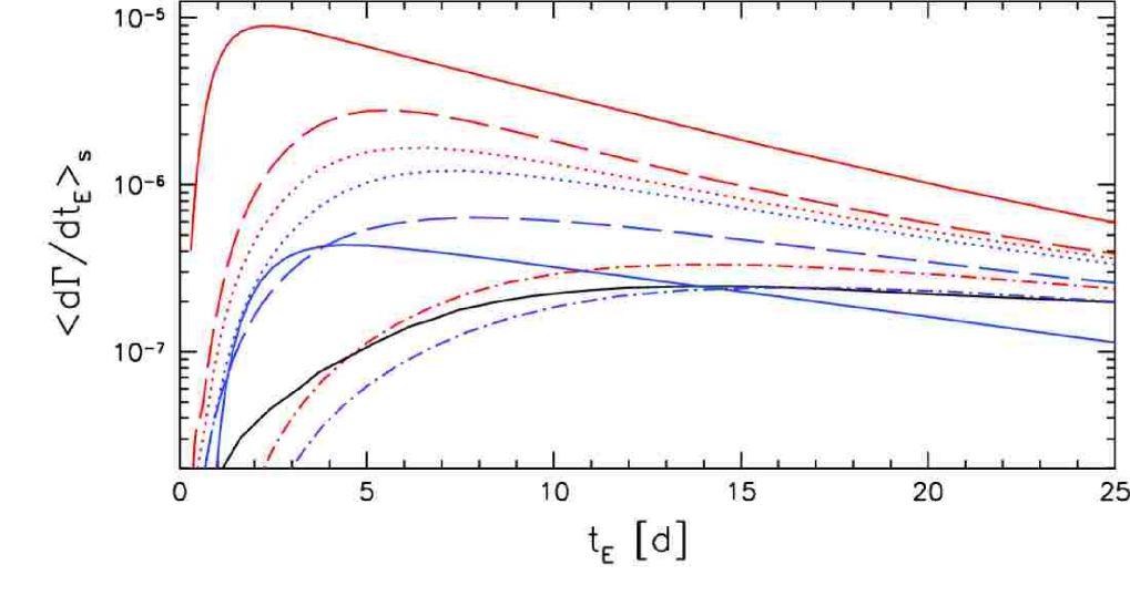
Figure 6.— Line-of-sight distance–averaged distribution of the event rate with Einstein timescale $\left<d\Gamma/d{t_{\mathrm{E}}}\right>_{s}$ ($\mathrm{yr}^{-1}$) using the model of M31 presented in § B and assuming a 100% MACHO halo. Results are shown for two positions in the intrinsic M31 coordinate system (see Figure 4), at $(x,y)=(1\arcmin,0\arcmin)$ (red), and at $(x,y)=(4.46\arcmin,4.46\arcmin)$ (corresponding to $(x,y)=(1\,\mathrm{kpc},1\,\mathrm{kpc})$, blue). The bulge-bulge Einstein time distribution is shown as solid line. The halo-bulge distributions have been evaluated for a MACHO mass of ${M}_{0}=0.1\,{{M}_{\odot}}$ (dotted line) and ${M}_{0}=0.5\,{{M}_{\odot}}$ (dot-dashed line). The halo-disk lensing case is shown for a MACHO mass of ${M}_{0}=0.1\,{{M}_{\odot}}$ (dashed line). The Einstein time distributions of the event rate differ considerably for halo-disk, halo-bulge and bulge-bulge lensing and also vary significantly with the line-of-sight position. For comparison we also plot the Einstein timescale distribution for M31 halo-lensing derived by Han & Gould (1996a) up to a pre-factor (that we chose equal to $3\times 10^{-6}$) as a black solid curve. Han & Gould (1996a) considered the distributions for the halo-disk and halo-bulge lensing to be similar and not distinguish between them further. They used a MACHO mass of ${M}_{0}=0.1\,{{M}_{\odot}}$ for their curve. However, it looks more similar to our halo-bulge curve for ${M}_{0}=0.5\,{{M}_{\odot}}$, and cannot be moved on the halo-bulge or halo-disk for ${M}_{0}=0.1\,{{M}_{\odot}}$ curve with another choice of the prefactor.

Figure 6 shows examples for this line-of-sight distance–averaged distribution $\left<d\Gamma_{\mathrm{T}}/d{t_{\mathrm{E}}}\right>_{s}$ for two different positions in the intrinsic M31 coordinate system (see Fig. 4), at $(x,y)=(1\arcmin,0\arcmin)$ and $(x,y)=(4.46\arcmin,4.46\arcmin)=(1\,\mathrm{kpc},1\,\mathrm{kpc})$. The distributions show a strong dependence on the line-of-sight position. The halo-bulge and halo-disk lensing timescales are longer than those of bulge-bulge lensing. An increase in MACHO mass decreases the event rate (see Fig. 5), and the timescale of the events becomes longer (see the examples for ${M}_{0}=0.1\,{{M}_{\odot}}$ and ${M}_{0}=0.5\,{{M}_{\odot}}$ in Fig. 6).

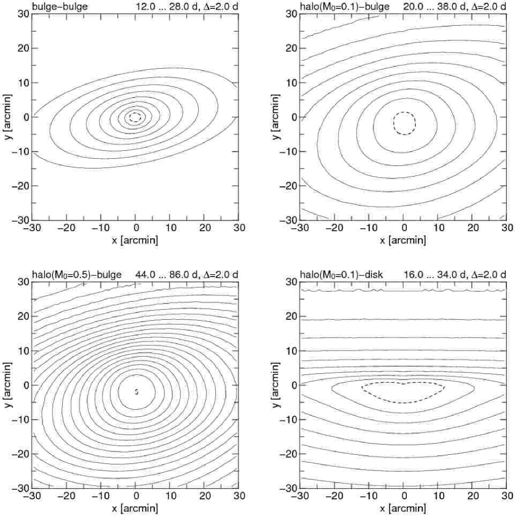
Figure 7.— Einstein timescale averaged over all sources $\overline{\left<{t_{\mathrm{E}}}\right>_{s}}$ calculated for lines of sights toward the center of M31 using the model of M31 presented in § B. We show the distributions for bulge-bulge self-lensing (first row, left), halo-bulge lensing for lenses of ${M}_{0}=0.1\,{{M}_{\odot}}$ [i.e., a mass function $\xi({M})=\delta({M}_{0}-0.1\,{{M}_{\odot}})/0.1\,{{M}_{\odot}}$] (first row, right), halo-bulge lensing for lenses of ${M}_{0}=0.5\,{{M}_{\odot}}$ (second row, left), and halo-disk lensing with ${{M}_{0}}=0.1\,{{M}_{\odot}}$ (second row, right). Contour levels and spacing are shown on top of each diagram. We assume the MACHO fraction in the dark halo to be unity. The dashed line marks the lowest contour level.

Weighting ${t_{\mathrm{E}}}$ with this function and integrating over all timescales finally yields the desired mean line-of-sight distance–averaged Einstein timescale of an event:

$$\overline{\left<{t_{\mathrm{E}}}\right>_{s}}\;:=\frac{\int\limits_{0}^{\infty}{t_{\mathrm{E}}}\left<\frac{d\Gamma}{d{t_{\mathrm{E}}}}\right>_{s}\,d{t_{\mathrm{E}}}}{\int\limits_{0}^{\infty}\left<\frac{d\Gamma}{d{t_{\mathrm{E}}}}\right>_{s}\,d{t_{\mathrm{E}}}}=\frac{2}{\pi}\frac{\left<\tau\right>_{s}}{\left<\Gamma_{1}\right>_{s}}\neq\left<\overline{{t_{\mathrm{E}}}}\right>_{s}.$$ (56)

Mean Einstein timescales $\overline{\left<{t_{\mathrm{E}}}\right>_{s}}$ are shown for lensing and self-lensing in Figure 7. Generally, the minimum of $\overline{\left<{t_{\mathrm{E}}}\right>_{s}}$ is near the M31 center, irrespective of the lens-source configuration. The mean Einstein timescale is smaller for lower MACHO masses, since the Einstein radii become smaller and are faster to cross (compare the two middle panels in Fig. 7). The bulge-bulge lensing events (first panel) are the shortest. This is caused by the small lens-source distances, which reduce the sizes of the Einstein radii.

5.4. The Amplification Distribution

The magnification distribution of the event rate is

$$\frac{d\Gamma}{d{A_{0}}}=\left|\frac{d{u_{0}}}{d{A_{0}}}\right|\frac{d\Gamma}{d{u_{0}}}=\left|\frac{d{u_{0}}}{d{A_{0}}}\right|\frac{\Gamma}{{u_{\mathrm{T}}}}.$$ (57)

Inserting equation (8) makes the result equal to that of Griest (1991).

Transforming equation (51) we can write

$$\frac{d^{2}\Gamma}{d{t_{\mathrm{E}}}\,d{A_{0}}}=\frac{2}{{t_{\mathrm{E}}}^{3}}\left|\frac{d{u_{0}}}{d{A_{0}}}\right|\int\limits_{0}^{\infty}\int\limits_{0}^{D_{\mathrm{os}}}\rho({D_{\mathrm{ol}}})\,\xi({M})\,{p_{v_{\mathrm{t}}}}{\left(\frac{{R_{\mathrm{E}}}}{{t_{\mathrm{E}}}}\right)}\,{R_{\mathrm{E}}}^{3}\,d{D_{\mathrm{ol}}}\,d{M}.\,$$ (58)

using $d{u_{0}}/d{A_{0}}$ from equation (8).

5.5. The Distribution for the FWHM Timescale

Although the Einstein timescale ${t_{\mathrm{E}}}$ contains all the relevant physical properties (mass, position, and velocity) of the lens, it is of limited practical use in the case of an ill-determined source flux (“Einstein time - magnification degeneracy”, see § 2.2). In this case ${t_{\mathrm{FWHM}}}$ is the only properly measurable timescale of a light curve. We obtain the distribution function for ${t_{\mathrm{FWHM}}}$ (neglecting finite-source effects), starting from § 3, using ${t_{\mathrm{FWHM}}}({v_{\mathrm{t}}},{M},{D_{\mathrm{ol}}},{u_{0}})=\frac{{R_{\mathrm{E}}}({M},{D_{\mathrm{ol}}})}{{v_{\mathrm{t}}}}w({u_{0}})$ (see eq. [9]):

$$\begin{array}[]{ll}\frac{d^{2}\Gamma}{d{t_{\mathrm{FWHM}}}\,d{u_{0}}}&=\int\limits_{0}^{\infty}\int\limits_{0}^{D_{\mathrm{os}}}\int\limits_{0}^{\infty}\,\rho({D_{\mathrm{ol}}})\,\xi({M})\,{p_{v_{\mathrm{t}}}}({v_{\mathrm{t}}})\,2{v_{\mathrm{t}}}\,{R_{\mathrm{E}}}\,\delta{\left({t_{\mathrm{FWHM}}}-\frac{{R_{\mathrm{E}}}}{{v_{\mathrm{t}}}}\,w({u_{0}})\right)}\,d{v_{\mathrm{t}}}\,d{D_{\mathrm{ol}}}\,d{M}\\ &=2\int\limits_{0}^{\infty}\int\limits_{0}^{D_{\mathrm{os}}}\int\limits_{0}^{\infty}\,\rho({D_{\mathrm{ol}}})\,\xi({M})\,{p_{v_{\mathrm{t}}}}({v_{\mathrm{t}}})\,{v_{\mathrm{t}}}{R_{\mathrm{E}}}\,\frac{\delta{\left({v_{\mathrm{t}}}-\frac{{R_{\mathrm{E}}}}{{t_{\mathrm{FWHM}}}}\,w({u_{0}})\right)}}{\left|-\frac{{R_{\mathrm{E}}}}{{v_{\mathrm{t}}}^{2}}\,w({u_{0}})\right|}\,d{v_{\mathrm{t}}}\,d{D_{\mathrm{ol}}}\,d{M}\\ &=\frac{2}{{t_{\mathrm{FWHM}}}^{3}}\int\limits_{0}^{\infty}\int\limits_{0}^{\infty}\,\rho({D_{\mathrm{ol}}})\,\xi({M})\,w^{2}({u_{0}})\,{R_{\mathrm{E}}}^{3}\,{p_{v_{\mathrm{t}}}}{\left(\frac{{R_{\mathrm{E}}}}{{t_{\mathrm{FWHM}}}}\,w({u_{0}})\right)}\,d{D_{\mathrm{ol}}}\,d{M}\\ &=\frac{2\,w^{2}({u_{0}})}{{t_{\mathrm{FWHM}}}^{3}}\int\limits_{0}^{\infty}\xi({M})\int\limits_{0}^{D_{\mathrm{os}}}\rho({D_{\mathrm{ol}}})\,{p_{v_{\mathrm{t}}}}{\left(\frac{{R_{\mathrm{E}}}}{{t_{\mathrm{FWHM}}}}\,w({u_{0}})\right)}\,{R_{\mathrm{E}}}^{3}\,d{D_{\mathrm{ol}}}\,d{M}.\end{array}$$ (59)

Baltz & Silk (2000) expressed the same relation in an alternative way and already motivated the same change of variables from ${v_{\mathrm{t}}}$ to ${t_{\mathrm{FWHM}}}$. Our relation for the FWHM time distribution of the event rate in equation (59) does not include any derivative or inversion of $w({u_{0}})$ and thus is very easy to evaluate numerically. Note that one can use $w(u_{0})\approx\sqrt{12}\,u_{0}$ as high-magnification approximation.

Replacing the relative impact parameter ${u_{0}}$ by the maximum amplification ${A_{0}}$ (using eqs. [7] and [8]) yields an equivalent description of this result:

$$\frac{d^{2}\Gamma}{d{t_{\mathrm{FWHM}}}\,d{A_{0}}}=\frac{2\Psi({A_{0}})}{{t_{\mathrm{FWHM}}}^{3}}\int\limits_{0}^{\infty}\xi({M})\int\limits_{0}^{D_{\mathrm{os}}}\rho({D_{\mathrm{ol}}})\,{p_{v_{\mathrm{t}}}}{\left(\frac{{R_{\mathrm{E}}}}{{t_{\mathrm{FWHM}}}}\,\Upsilon({A_{0}})\right)}\,{R_{\mathrm{E}}}^{3}\,d{D_{\mathrm{ol}}}\,d{M},$$ (60)

with ${R_{\mathrm{E}}}({M},{D_{\mathrm{ol}}},{D_{\mathrm{os}}})$ and $\Psi({A_{0}})$ as

$$\Psi({A_{0}}):=\left|\frac{d{u_{0}}}{d{A_{0}}}\right|\,\Upsilon^{2}({A_{0}})=4\sqrt{2}\,\frac{\left[{A_{0}}+({A_{0}}^{2}-1)^{1/2}\right]^{1/2}\,\left[({A_{0}}+1)^{3/2}-{A_{0}}({A_{0}}+3)^{1/2}\right]}{({A_{0}}^{2}-1)^{7/4}({A_{0}}+3)^{1/2}}\stackrel{{\scriptstyle{A_{0}}\gg 1}}{{\approx}}\frac{12}{{A_{0}}^{4}},$$ (61)

where $\left|\frac{d{u_{0}}}{d{A_{0}}}\right|$ was defined in equation (8).

Figure 8 shows the distribution of events $\left<\frac{d^{2}\Gamma}{d\log({t_{\mathrm{FWHM}}}/[d])\,d\log{A_{0}}}\right>_{s}$, at the position $(x,y)=(1\arcmin,0\arcmin)$ in the intrinsic M31 coordinate system (see Fig. 4), i.e., on the disk major axis.

Small amplifications are favored, which implies a strong dependency of the total number of events on the experimental limit of ${A_{0}}$ (e.g., $A_{\mathrm{T}}$). Figure 8 can be compared with sensitivity regions of current experimental setups for microlensing experiments toward M31. As these are usually only sensitive to ${t_{\mathrm{FWHM}}}$ of larger than 1 day, it is extremely unlikely to detect maximum magnifications larger than $10^{3}$. These high-magnification events can only be routinely detected with combined observations from several sights located on different longitudes, with large telescopes allowing short integration times, or from space. Note that recently after an alert detection and intensive follow-up monitoring, Dong et al. (2006) could measure a lensing time-scale of ${t_{\mathrm{FWHM}}}\approx 0.05\,\mathrm{d}$ and a magnification of the order 3000.

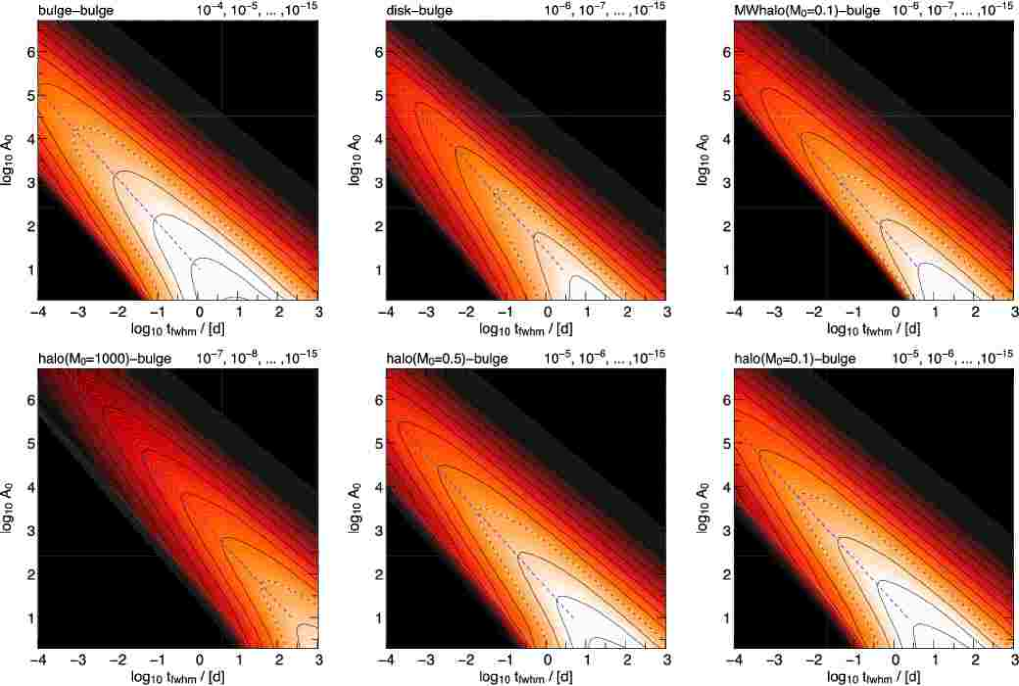
Figure 8.— Distribution $\left<d^{2}\Gamma/\left(d\log{t_{\mathrm{FWHM}}}\,d\log{A_{0}}\right)\right>_{s}$ (y^-1) (i.e., rate per year and line-of-sight) for different lens-source configurations, calculated at the position $(x,y)=(1\arcmin,0\arcmin)$ in the intrinsic M31 coordinate system (see Fig. 4). The values of timescale and magnification are largely confined to a linear region within the logarithmic timescale-magnification plane. First row, left panel: Bulge-bulge lensing; middle panel: disk-bulge lensing; right panel: MW-halo-bulge lensing for MW lenses with ${{M}_{0}}=0.1\,{{M}_{\odot}}$. Second row, left panel: Halo-bulge lensing with ${{M}_{0}}=1000\,{{M}_{\odot}}$; middle panel: halo-bulge lensing with ${{M}_{0}}=0.5\,{{M}_{\odot}}$; right panel: halo-bulge lensing with ${{M}_{0}}=0.1\,{{M}_{\odot}}$. The dashed contour level line marks the $10^{-8}$ (y^-1) level in each diagram. The number of events rises toward smaller amplifications and larger timescales. Small amplifications are strongly favored for all lens-source configurations. The number of high-amplification events rises for smaller ${t_{\mathrm{FWHM}}}$ timescale. Detecting events toward M31 with maximum amplifications of ${A_{0}}>10^{3}$ therefore requires an experiment that is particularly sensitive to short timescale events. The dashed blue line shows for each selected timescale the amplification where the distribution is maximal [$\partial\log({A_{0}})=0$].

6. Applications for the Pixel-Lensing Regime

The microlensing parameters (${F_{0}}$, ${t_{\mathrm{E}}}$, and ${u_{0}}$) are not directly observable anymore in crowded or unresolved stellar fields. In that case, the two measurable quantities are the full-width timescale ${t_{\mathrm{FWHM}}}$ and the difference flux ${\Delta_{F}}$ of an event.

We now make use of the luminosity function $\tilde{\Phi}({\mathcal{M}})$, the source number density $n_{s}(x,y,{D_{\mathrm{os}}})$, and the color distribution ${p_{\mathrm{cmd}}}({\mathcal{M}},{\mathcal{C}})$ of the source stars introduced in § 4 and derive the event rate distribution function $\frac{d^{2}\Gamma}{d{t_{\mathrm{FWHM}}}\,d{\Delta_{F}}}$. This quantity can then be linked to the measured distributions most straightforwardly.

In the first two subsections (§§ 6.1 and 6.2) we derive the required distributions neglecting finite source effects. However, the high magnifications needed to boost MS stars to large flux excesses go in parallel with finite source effects that make these large flux excesses hardly possible. We show this in detail in § 6.3, where we incorporate finite source effects in the calculations.

6.1. Changing Variables of $\Gamma$ to ${t_{\mathrm{FWHM}}}$ and ${\Delta_{F}}$

6.1.1 Event Rate per Star with Absolute Magnitude ${\mathcal{M}}$

We now use the relations ${R_{\mathrm{E}}}({M},{D_{\mathrm{ol}}},{D_{\mathrm{os}}})$, ${A_{0}}({F_{0}},{\Delta_{F}})$, ${t_{\mathrm{FWHM}}}({v_{\mathrm{t}}},{R_{\mathrm{E}}},b)$, $\Psi[{A_{0}}({F_{0}},{\Delta_{F}})]$, and $\Upsilon[{A_{0}}({F_{0}},{\Delta_{F}})]$ from § 2 and the equations ${t_{\mathrm{FWHM}}}({v_{\mathrm{t}}},{R_{\mathrm{E}}},{F_{0}},{\Delta_{F}})=\frac{{R_{\mathrm{E}}}}{{v_{\mathrm{t}}}}\,\Upsilon({A_{0}})$, ${\Delta_{F}}({F_{0}},b,{R_{\mathrm{E}}})={F_{0}}\left[A(b/{R_{\mathrm{E}}})-1\right]$ and $\frac{d{\Delta_{F}}}{db}=-8\frac{{F_{0}}}{{R_{\mathrm{E}}}}\,{u_{0}}^{-2}\,\left[{u_{0}}^{2}+4\right]^{-3/2}\,,$ and we obtain the event rate per FWHM time, per flux excess, per lens mass and per source star with an absolute magnitude ${\mathcal{M}}$:

$$\begin{array}[]{rl}\frac{d^{4}\Gamma}{d{t_{\mathrm{FWHM}}}\,d{\Delta_{F}}\,d{M}\,d{\mathcal{M}}}&=\tilde{\Phi}({\mathcal{M}})\int\limits_{0}^{D_{\mathrm{os}}}\int\limits_{0}^{\infty}\int\limits_{0}^{\infty}\frac{d^{4}\Gamma}{d{D_{\mathrm{ol}}}\,d{M}\,d{v_{\mathrm{t}}}\,db}\,\delta{\left\{{\Delta_{F}}-{F_{0}}\left[A\left(\frac{b}{{R_{\mathrm{E}}}}\right)-1\right]\right\}}\,\delta{\left\{{t_{\mathrm{FWHM}}}-\frac{{R_{\mathrm{E}}}}{{v_{\mathrm{t}}}}\,w\right\}}\,db\,d{v_{\mathrm{t}}}\,d{D_{\mathrm{ol}}}\\ &=\tilde{\Phi}\int\limits_{0}^{D_{\mathrm{os}}}\int\limits_{0}^{\infty}\int\limits_{0}^{\infty}\rho\,\xi\,{p_{v_{\mathrm{t}}}}\,2{v_{\mathrm{t}}}\,\frac{\delta{\left\{b-{R_{\mathrm{E}}}\left[2{A_{0}}({A_{0}}^{2}-1)^{-1/2}-2\right]^{1/2}\right\}}}{\left|\frac{d{\Delta_{F}}}{db}\right|}\,\delta{\left({t_{\mathrm{FWHM}}}-\frac{{R_{\mathrm{E}}}}{{v_{\mathrm{t}}}}\,\omega\right)}\,db\,d{v_{\mathrm{t}}}\,d{D_{\mathrm{ol}}}\\ &=2\tilde{\Phi}\frac{1}{{F_{0}}}\frac{d{u_{0}}}{d{A_{0}}}\int\limits_{0}^{D_{\mathrm{os}}}\int\limits_{0}^{\infty}\rho\,\xi\,{p_{v_{\mathrm{t}}}}\,{v_{\mathrm{t}}}\,{R_{\mathrm{E}}}\,\delta{\left({t_{\mathrm{FWHM}}}-\frac{{R_{\mathrm{E}}}}{{v_{\mathrm{t}}}}\,\Upsilon\right)}\,d{v_{\mathrm{t}}}\,d{D_{\mathrm{ol}}}\\ &=2\tilde{\Phi}\frac{1}{{F_{0}}}\frac{d{u_{0}}}{d{A_{0}}}\int\limits_{0}^{D_{\mathrm{os}}}\int\limits_{0}^{\infty}\rho\,\xi\,{p_{v_{\mathrm{t}}}}\,{v_{\mathrm{t}}}\,{R_{\mathrm{E}}}\,\frac{\delta{\left({v_{\mathrm{t}}}-\frac{{R_{\mathrm{E}}}}{{t_{\mathrm{FWHM}}}}\,\Upsilon\right)}}{\left|-\frac{{R_{\mathrm{E}}}}{{v_{\mathrm{t}}}^{2}}\Upsilon\right|}\,d{v_{\mathrm{t}}}\,d{D_{\mathrm{ol}}}\\ &=2\tilde{\Phi}\frac{1}{{F_{0}}}\frac{d{u_{0}}}{d{A_{0}}}\,\Upsilon^{2}\,\frac{1}{{t_{\mathrm{FWHM}}}^{3}}\int\limits_{0}^{D_{\mathrm{os}}}\rho\,\xi\,{p_{v_{\mathrm{t}}}}{\left(\frac{{R_{\mathrm{E}}}}{{t_{\mathrm{FWHM}}}}\,\Upsilon\right)}\,{R_{\mathrm{E}}}^{3}\,d{D_{\mathrm{ol}}}\\ &=\frac{2}{{t_{\mathrm{FWHM}}}^{3}}\,\tilde{\Phi}({\mathcal{M}})\,\xi({M})\,\frac{\Psi}{{F_{0}}}\int\limits_{0}^{D_{\mathrm{os}}}\rho({D_{\mathrm{ol}}})\,{R_{\mathrm{E}}}^{3}\,{p_{v_{\mathrm{t}}}}{\left(\frac{{R_{\mathrm{E}}}}{{t_{\mathrm{FWHM}}}}\,\Upsilon\right)}\,d{D_{\mathrm{ol}}}.\end{array}$$ (62)

using the luminosity function in magnitudes $\tilde{\Phi}({\mathcal{M}})$ and the conversion from absolute magnitudes to intrinsic source fluxes ${F_{0}}({\mathcal{M}},{D_{\mathrm{os}}})$ (eq. [42]). Equation (62) is the transformation of equation (32) to the observables relevant in the pixel-lensing regime. It gives the event rate per star with absolute magnitude ${\mathcal{M}}$ and will be converted to the event rate per area using the density of stars below. For the special case of highly amplified events, (${A_{0}}\gg 1$), the approximations $\Psi\approx 12({F_{0}}/{\Delta_{F}})^{4}$ and $\Upsilon\approx\sqrt{12}({F_{0}}/{\Delta_{F}})$ can be inserted into equation (62).

6.1.2 Event Rate per Area

All previously derived event rates are per star, or per star with a given absolute magnitude ${\mathcal{M}}$. Observed, however, are event rates per area. These are obtained from the source density distribution along the line-of-sight $n_{s}(x,y,{D_{\mathrm{os}}})$ and equation (62):

$$\frac{d^{6}\Gamma_{s,l}}{dx\,dy\,d{t_{\mathrm{FWHM}}}\,d{\Delta_{F}}\,d{M}\,d{\mathcal{M}}}=\frac{2\,\tilde{\Phi}_{s}({\mathcal{M}})\,\xi_{l}({M})}{{t_{\mathrm{FWHM}}}^{3}}\int\limits_{0}^{\infty}n_{s}(x,y,{D_{\mathrm{os}}})\,\frac{\Psi}{{F_{0}}}\int\limits_{0}^{D_{\mathrm{os}}}\rho_{l}({D_{\mathrm{ol}}})\,{R_{\mathrm{E}}}^{3}\,{p_{v_{\mathrm{t}}}}{\left(\frac{{R_{\mathrm{E}}}\Upsilon}{{t_{\mathrm{FWHM}}}},v_{0}\right)}\,d{D_{\mathrm{ol}}}\,d{D_{\mathrm{os}}},$$ (63)

where the quantities in the integral have the following functional dependences ${F_{0}}({\mathcal{M}},{D_{\mathrm{os}}})$, $\rho_{l}(x,y,{D_{\mathrm{ol}}})$, ${R_{\mathrm{E}}}({D_{\mathrm{ol}}},{M},{D_{\mathrm{os}}})$, $\Psi({A_{0}}({F_{0}},{\Delta_{F}}))$, $\Upsilon({A_{0}}({F_{0}},{\Delta_{F}}))$, $v_{0}(x,y,{D_{\mathrm{ol}}},{D_{\mathrm{os}}})$. Equation (63) is the event rate per interval of lens plane area, FWHM time flux excess, lens mass and absolute magnitude of the lensed star. For highly amplified events one can replace $\Psi$ and $\Upsilon$ in the integral by $12({F_{0}}/{\Delta_{F}})^{4}$ and $\sqrt{12}({F_{0}}/{\Delta_{F}})$, respectively.

Different lens (disk, bulge, or halo) and source (disk or bulge) populations are characterized by an index $l$ and $s$ in equation (63). For the total event rate $\Gamma_{\rm tot}$ one has to sum up the contributions of all lens-source configurations:

$$\frac{d^{6}\Gamma_{\mathrm{tot}}}{\,dx\,dy\,d{t_{\mathrm{FWHM}}}\,d{\Delta_{F}}\,d{M}\,d{\mathcal{M}}}:=\sum\limits_{s}\sum\limits_{l}\frac{d^{6}\Gamma_{s,l}}{dx\,dy\,d{t_{\mathrm{FWHM}}}\,d{\Delta_{F}}\,d{M}\,d{\mathcal{M}}}.$$ (64)

The event rate per area is then obtained by multiplying equation (64) with the efficiency ${\epsilon}(x,y,{\Delta_{F}},{t_{\mathrm{FWHM}}})$ of the experiment and integrating over all lens masses and source magnitudes, and the timescale and flux excess. The probability that one can observe two stars lensed at the same time at the same position is practically zero, since $\int_{\Omega_{\mathrm{psf}}}(d^{2}\Gamma_{\rm tot}/dx\,dy)\;dx\;dy\ll 1$ holds.

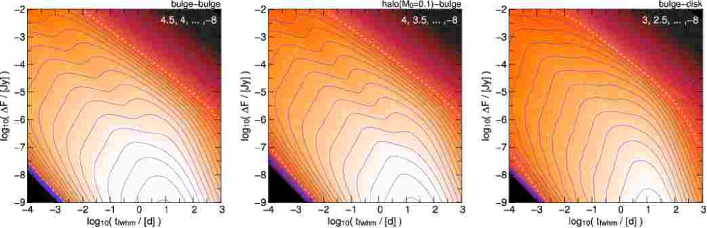
Figure 9.— Event rate per area, per FWHM time and per flux excess, $d^{4}\Gamma/(dx\;dy\;d\log{t_{\mathrm{FWHM}}}\,\,d\log{\Delta_{F}})$, obtained from equation (63) by mass and magnitude integration. The contours are shown in units of $\mathrm{y}^{-1}\,\mathrm{arcmin}^{-2}$, timescales and flux excess have been inserted in units of $\mathrm{days}$ and $\mathrm{Jy}$. The equations are evaluated at $(x,y)=(1\arcmin,0\arcmin)$ in the intrinsic M31 coordinate system (see Figure 4), i.e., at a distance of $1\arcmin$ along the disk major axis. We show bulge-bulge lensing (left), halo-bulge lensing with ${{M}_{0}}=0.1\,{{M}_{\odot}}$ lenses, and bulge-disk lensing (right). The contour levels are given as inserts in each diagram. The red dashed line marks the $10^{-3}\,\mathrm{y}^{-1}\,\mathrm{arcmin}^{-2}$ level in each diagram, brighter areas correspond to higher values. The double-wave shape of the contours with bulge stars as sources is caused by the shape of the PMS luminosity function of the bulge sources (see Figure 10). For the results shown in these panels all sources have been treated as point sources. For finite source effects, see § 6.3.

We carry out mass and magnitude integration of equation (63) for the position $(x,y)=(1\arcmin,0\arcmin)$ in the intrinsic M31 coordinate system (see Figure 4), i.e., at a distance of $0.22\,\mathrm{kpc}$ along the disk major axis and show the results for bulge-bulge, halo-bulge, and bulge-disk lensing in Figure 9. Compared to Figure 8 the contours are smeared out in the $\Delta F$-direction, since they come from convolving those in Figure 8 with the source luminosity function.

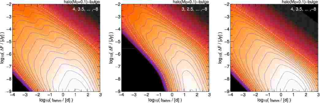
Figure 10.— Event rate per area, per FWHM time and per flux excess, $d^{4}\Gamma/dx\;dy\;d\log{t_{\mathrm{FWHM}}}\,\,d\log{\Delta_{F}})$, for halo-bulge lensing with ${{M}_{0}}=0.1\,{{M}_{\odot}}$ calculated at the position $(x,y)=(1,0)\,\mathrm{arcmin}$. Left panel: Distribution for PMS and MS sources. Middle panel: Distribution for PMS sources alone. Right panel: Distribution for MS sources alone. The contour levels are shown as inserts in each diagram. The red line marks the $10^{-3}\,\mathrm{y}^{-1}\,\mathrm{arcmin}^{-2}$ level in each diagram. The double -wave shape of the PMS distribution is due to the two peaks in the PMS luminosity function of the bulge sources (see Figure 25 in § B). For the results shown in these panels all sources have been treated as point sources.

In Figure 10 we demonstrate for the halo-bulge lensing case in Figure 9 that the “double-wave shape” in the contours in the two left panels of Figure 9 indeed is caused by the luminosity function of the PMS stars. We split the source stars into post–main-sequence (PMS) and main-sequence (MS) stars and plot the corresponding contours into the middle and right panels of that figure. The double-wave shape appears only in the PMS figure. Besides that, it becomes obvious that PMS stars cannot be lensed into events with short timescales and small flux excess. This is because the faintest PMS stars in the M31 bulge have an unamplified flux of $8\times\,10^{-9}\,\mathrm{Jy}$ and thus need an amplification of only a factor of $2$ to yield a flux excess of ${\Delta_{F}}\approx 10^{-8}\,\mathrm{Jy}$. Magnifications that small are incompatible with short timescales according to Figure 8. In contrast, MS stars need very high amplifications to reach a flux excess comparable to that typical for PMS stars. According to the right panel in Figure 10, ultra-short, large excess flux events with MS source stars would be more common [compare, e.g., the contour levels at $\log({t_{\mathrm{FWHM}}}/[\mathrm{d}])=-3$ and $\log(\Delta F/[\mathrm{Jy}])={-4}$] than events with PMS source stars.

6.2. Including Color Information in the Event Rate

The color of a point source remains unchanged during a lensing event, since the lensing amplification does not depend on the frequency of the source light. In practice, microlensing events with blending by nearby stars, and any event with finite source signatures may show chromaticity in the light curve (see e.g. Valls-Gabaud (1995); Witt (1995); Han et al. (2000)). The difference imaging technique eliminates all blended light from the lensing light curve. For lensing events without finite source effects the color of the event therefore equals that of the source and can be used to constrain the source-star luminosities.

Replacing $\tilde{\Phi}({\mathcal{M}})$ with ${p_{\mathrm{cmd}}}({\mathcal{M}},{\mathcal{C}})$, and $d{\mathcal{M}}$ with $\,d{\mathcal{M}}\,d{\mathcal{C}}$ (see § 4.4), we obtain

$$\frac{d^{7}\Gamma_{s,l}}{\,dx\,dy\,d{t_{\mathrm{FWHM}}}\,d{\Delta_{F}}\,d{M}\,d{\mathcal{M}}\,d{\mathcal{C}}}=\frac{2}{{t_{\mathrm{FWHM}}}^{3}}\,{p_{\mathrm{cmd}}}_{s}({\mathcal{M}},{\mathcal{C}})\,\xi_{l}({M})\int\limits_{0}^{\infty}n_{s}(x,y,{D_{\mathrm{os}}})\,\frac{\Psi}{{F_{0}}}\int\limits_{0}^{D_{\mathrm{os}}}\rho_{l}({D_{\mathrm{ol}}})\,{R_{\mathrm{E}}}^{3}\,{p_{v_{\mathrm{t}}}}{\left(\frac{{R_{\mathrm{E}}}\Upsilon}{{t_{\mathrm{FWHM}}}},v_{0}\right)}\,d{D_{\mathrm{ol}}}\,d{D_{\mathrm{os}}}.$$ (65)

We derive lens mass estimates starting from equation (65) in § 8. We also demonstrate there that including the color information leads to considerably smaller allowed lens mass intervals than for the case in which color information is ignored (i.e., the case in which lens mass probability functions are derived from eq. [63]).

Equation (65) allows to reconstruct the mass function of the lenses and the MACHO fraction in the dark halo (see de Rujula et al. (1991); Jetzer & Massó (1994); Jetzer (1994); Mao & Paczyński (1996); Han & Gould (1996b); Gould (1996a)). In this way one can obtain the optimal parameterization for the mass function $\xi_{l}({M})$ using a maximum-likelihood analysis for a set of measured lensing events. If the ingredients for the kernel (i.e., all but the pre-factor $\xi_{l}({M})$ in eq. [65]) are accurately provided by theory and the number of lensing events is large, then the mass distribution can be derived solving the Fredholm integral equation of the first kind. Inversely, a certain ensemble of lenses allows conclusions on the based distribution functions.

6.3. Event Rate Taking into Account Finite Source Effects

As described in § 2.1 the point-source approximation is no longer valid, if the impact parameter ${u_{0}}$ is smaller than ${u_{0}^{\ast}}$, i.e., half the source radius projected onto the lens plane (equation (14)). In this case, the maximum amplification and thus the flux excess stays below the value for the point-source approximation, and timescales of events are enlarged (see Eqs. 16 and 13). Baltz & Silk (2000) already accounted for the upper limit in magnification and obtained the correct value for the total number of events (i.e., events with and without finite source signatures) as a function of magnification threshold. Their approximation, however, is limited to high amplifications and ignores the change of magnification and event timescale. Thus, the flux excess and timescale distributions of the events are not predicted accurately.

We have shown in § 2.1 that finite source effects are likely already for small maximal magnifications and that the timescale changes due to finite source effects can be large. Therefore, we derive precise relations and account for the finite source sizes as follows:

1. Events with ${u_{0}}>{u_{0}^{\ast}}$, i.e., those for which the finite source sizes are irrelevant, are treated as before; we redo all calculations starting from equation (31), and if the impact parameter $b$ is involved in an integral we multiply the integrand with $\theta{\left(b-{R_{\mathrm{E}}}{u_{0}^{\ast}}\right)}$; the step function allows only contributions in the integrand, if $b\geq{R_{\mathrm{E}}}{u_{0}^{\ast}}$ holds. To see how this transports into the $d{D_{\mathrm{ol}}}$-integration if the variables are changed from $b$ and ${v_{\mathrm{t}}}$ to ${t_{\mathrm{FWHM}}}$ and $\Delta F$ in the Eqs. 62, 63 and 65

$$\theta{\left(b-{R_{\mathrm{E}}}{u_{0}^{\ast}}\right)}=\theta{\left({A_{0}^{\ast}}-{A_{0}}\right)}=\theta{\left({D_{\mathrm{os}}}\left\{1+\frac{c^{2}\,R_{\ast}^{2}\frac{{\Delta_{F}}}{{F_{0}}}\left(2+\frac{{\Delta_{F}}}{{F_{0}}}\right)}{16\,G{M}\,{D_{\mathrm{os}}}}\right\}^{-1}-{D_{\mathrm{ol}}}\right)}=\theta{\left({D_{\mathrm{ol}}^{\ast}}-{D_{\mathrm{ol}}}\right)}$$ (66)

where we are using the following relations:

$${D_{\mathrm{ol}}^{\ast}}:={D_{\mathrm{os}}}\left(1+\frac{{\Delta_{F}}(2{F_{0}}+{\Delta_{F}})}{{C_{D_{\mathrm{ol}}^{\ast}}}\,{D_{\mathrm{os}}}}\right)^{-1}\approx{D_{\mathrm{os}}}\left(1+\frac{{\Delta_{F}}^{2}}{{C_{D_{\mathrm{ol}}^{\ast}}}\,{D_{\mathrm{os}}}}\right)^{-1},$$

and

$${C_{D_{\mathrm{ol}}^{\ast}}}:=\frac{16\,{F_{0}}^{2}\,G{M}}{c^{2}\,R_{\ast}^{2}}\,\left(\mathrm{flux}^{2}\,\mathrm{length}^{-1}\right).$$

Multiplying the integrand of equations (62), (63), and (65) with equation (66) extracts only those light curves, where finite-source effects can be neglected.

2. For events where the finite source sizes are relevant, i.e., events with ${u_{0}}<{u_{0}^{\ast}}$, we use the approximations for the maximum amplification and the FWHM time given in equations (15) and (16). This means that we just replace the relations for the impact parameter and the maximum magnification and the FWHM timescale relations of events by equations (13) and (16) when switching from the point source to the finite source regime. We then can derive the equations for the event rates with finite source effects from equation (32) analogously to the point-source approximation, but this time with a step function of $\theta{\left({R_{\mathrm{E}}}{u_{0}^{\ast}}-b\right)}$ in the integrands allowing only small impact parameters. With ${A_{0}^{\ast}}({D_{\mathrm{ol}}},{D_{\mathrm{os}}},R_{\ast},{M})$, ${u_{0}^{\ast}}({D_{\mathrm{ol}}},{D_{\mathrm{os}}},R_{\ast},{M})$ and ${v_{\mathrm{t}}}=\left({R_{\mathrm{E}}}/{t_{\mathrm{FWHM}}}\right){\Upsilon^{\ast}}({A_{0}^{\ast}},{u_{0}})$ and its derivative $\left|d{t_{\mathrm{FWHM}}}({v_{\mathrm{t}}})/d{v_{\mathrm{t}}}\right|=\left({R_{\mathrm{E}}}/{v_{\mathrm{t}}}^{2}\right){\Upsilon^{\ast}}$ we obtain

$$\begin{array}[]{rl}\frac{d^{6}\Gamma_{s,l}}{\,dx\,dy\,d{t_{\mathrm{FWHM}}}\,d{\Delta_{F}}\,d{M}\,d{\mathcal{M}}}=&\int\limits_{0}^{\infty}n_{s}(x,y,{D_{\mathrm{os}}})\,\tilde{\Phi}_{s}({\mathcal{M}})\int\limits_{0}^{D_{\mathrm{os}}}\int\limits_{0}^{\infty}\int\limits_{0}^{\infty}\frac{d^{4}\Gamma}{d{D_{\mathrm{ol}}}\,d{M}\,d{v_{\mathrm{t}}}\,db}\,\delta{\left({\Delta_{F}}-{F_{0}}({A_{0}^{\ast}}-1)\right)}\\ &\times\,\delta{\left({t_{\mathrm{FWHM}}}-\frac{{R_{\mathrm{E}}}}{{v_{\mathrm{t}}}}{\Upsilon^{\ast}}\right)}\,\theta\left({R_{\mathrm{E}}}{u_{0}^{\ast}}-b\right)\,db\,d{v_{\mathrm{t}}}\,d{D_{\mathrm{ol}}}\,d{D_{\mathrm{os}}}\\ =&\int\limits_{0}^{\infty}n_{s}(x,y,{D_{\mathrm{os}}})\,\tilde{\Phi}_{s}({\mathcal{M}})\int\limits_{0}^{D_{\mathrm{os}}}\rho({D_{\mathrm{ol}}})\int\limits_{0}^{\infty}\int\limits_{0}^{\infty}\,\xi({M})\,{p_{v_{\mathrm{t}}}}({v_{\mathrm{t}}})\,2{v_{\mathrm{t}}}\\ &\times\,\delta{\left({\Delta_{F}}-{F_{0}}({A_{0}^{\ast}}-1)\right)}\,\frac{\delta{\left({v_{\mathrm{t}}}-({R_{\mathrm{E}}}/{t_{\mathrm{FWHM}}}){\Upsilon^{\ast}}\right)}}{({R_{\mathrm{E}}}/{v_{\mathrm{t}}}^{2}){\Upsilon^{\ast}}}\,\theta\left({R_{\mathrm{E}}}{u_{0}^{\ast}}-b\right)\,d{v_{\mathrm{t}}}\,db\,d{D_{\mathrm{ol}}}\,d{D_{\mathrm{os}}}\\ =&\int\limits_{0}^{\infty}n_{s}\,2\,\tilde{\Phi}_{s}({\mathcal{M}})\int\limits_{0}^{D_{\mathrm{os}}}\rho({D_{\mathrm{ol}}})\,\xi({M})\,\delta{\left({\Delta_{F}}-{F_{0}}({A_{0}^{\ast}}-1)\right)}\int\limits_{0}^{{R_{\mathrm{E}}}{u_{0}^{\ast}}}\,{p_{v_{\mathrm{t}}}}{\left(\frac{{R_{\mathrm{E}}}}{{t_{\mathrm{FWHM}}}}{\Upsilon^{\ast}}\right)}\,\frac{{R_{\mathrm{E}}}^{2}{{\Upsilon^{\ast}}}^{2}}{{t_{\mathrm{FWHM}}}^{3}}\,db\,d{D_{\mathrm{ol}}}\,d{D_{\mathrm{os}}}\\ =&\int\limits_{0}^{\infty}n_{s}(x,y,{D_{\mathrm{os}}})\frac{2}{{t_{\mathrm{FWHM}}}^{3}}\,\tilde{\Phi}_{s}({\mathcal{M}})\,\xi({M})\,\rho({D_{\mathrm{ol}}^{\ast}})\,{\Omega^{\ast}}\,{R_{\mathrm{E}}}({D_{\mathrm{ol}}^{\ast}})^{3}\int\limits_{0}^{{u_{0}^{\ast}}}\,{p_{v_{\mathrm{t}}}}{\left(\frac{{R_{\mathrm{E}}}({D_{\mathrm{ol}}^{\ast}})}{{t_{\mathrm{FWHM}}}}{\Upsilon^{\ast}}\right)}\,{{\Upsilon^{\ast}}}^{2}\,d{u_{0}}\,d{D_{\mathrm{os}}},\end{array}$$ (67)

with

$${\Omega^{\ast}}:=\left|\frac{d{D_{\mathrm{ol}}^{\ast}}({\Delta_{F}},{D_{\mathrm{os}}})}{d{\Delta_{F}}}\right|=2{C_{D_{\mathrm{ol}}^{\ast}}}{D_{\mathrm{os}}}^{2}({F_{0}}+{\Delta_{F}})\left({C_{D_{\mathrm{ol}}^{\ast}}}{D_{\mathrm{os}}}+{\Delta_{F}}(2{F_{0}}+{\Delta_{F}})\right)^{-2}\approx 2{C_{D_{\mathrm{ol}}^{\ast}}}{D_{\mathrm{os}}}^{2}{\Delta_{F}}\left({C_{D_{\mathrm{ol}}^{\ast}}}{D_{\mathrm{os}}}+{\Delta_{F}}^{2}\right)^{-2}.$$

Alternatively a transformation inverting ${t_{\mathrm{FWHM}}}(b)$ is possible. We use the values for the source radius, luminosity, and color relations $R_{\ast}({\mathcal{M}},{\mathcal{C}})$ summarized in Appendix B (§§ B.3 and B.4).

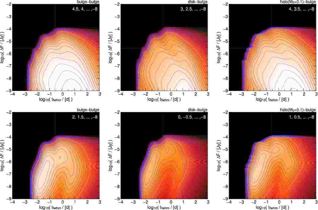
Figure 11.— $d^{2}\Gamma/\left(d\log{t_{\mathrm{FWHM}}}\,d\log{\Delta_{F}}\right)$ [$\,\mathrm{arcmin^{-2}}\,\mathrm{y^{-1}}$] at $(x,y)=(1\arcmin,0\arcmin)$ in the $\log({\Delta_{F}})$-$\log({t_{\mathrm{FWHM}}})$ plane, for bulge-bulge (left), disk-bulge (middle), and halo-bulge (right) lensing with $0.1\,{{M}_{\odot}}$ MACHOs (columns 1-3). The upper panels show the distribution for light curves not affected by the finite source sizes. The contours have been obtained from inserting eq. (63) into eq. (66) and carrying out the mass and source luminosity integral. The lower panels show the distribution for light curves with finite source signatures (mass and source star luminosity integral of eq. (67). The contour levels can be read off from the inserts in each diagram. The dashed line marks the $10^{-3}\,\mathrm{arcmin}^{-2}\,\mathrm{y}^{-1}$ level, areas with brighter colors correspond to higher contour values. Taking into account the finite source sizes implies an upper limit for ${\Delta_{F}}$ and a lower limit for ${t_{\mathrm{FWHM}}}$ for all light curves, i.e., for light curves with and with out finite source signatures (see text). For the source-lens configurations shown here there are no lensing eventslight curves with excess fluxes ${\Delta_{F}}>5\times 10^{-4}\,\mathrm{Jy}$. The results shown here have been obtained by taking into account the source sizes of lensed stars.

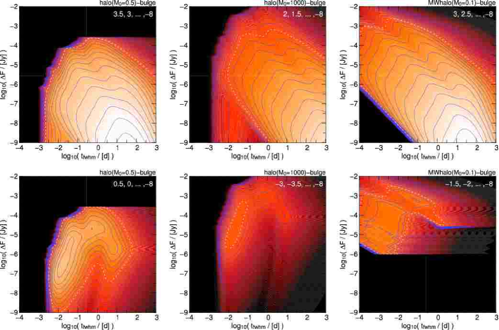
Figure 12.— Same as Fig. 11 for halo-bulge lensing with larger MACHO masses ($0.5\,{{M}_{\odot}}$ and $1000\,{{M}_{\odot}}$ MACHOs in the first and second column) and for Milky Way halo - M31 bulge lensing (for $0.1\,{{M}_{\odot}}$ MACHOs in the third column) As before, the dashed line marks the $10^{-3}\,\mathrm{arcmin}^{-2}\,\mathrm{y}^{-1}$ level in each diagram, and areas with brighter colors correspond to contour higher values. The results shown here have been obtained by taking into account the source sizes of lensed stars.

Figures 11 and 12 show contours of the event rate per ${t_{\mathrm{FWHM}}}$ timescale and flux excess, per year and square arcminute, with finite source effects taken into account. We use the same position as before, at $(x,y)=(1\arcmin,0\arcmin)$ in the intrinsic M31 coordinate system (see Figure 4) or at a disk major axis distance of $1\arcmin$. The upper panels show the distribution for light curves showing no finite source effects (eq. [63] with eq. [66]), whereas the lower panels show the distribution obtained from mass and source luminosity integration of equation (67), i.e., for light curves affected by finite source effects.

The black areas indicate the event parameter space, which is not available to source stars once their real sizes are taken into account: as finite source effects mainly occur at large amplifications, large ${\Delta_{F}}$ and small ${t_{\mathrm{FWHM}}}$ values are suppressed. Events in the point-source approximation, which fall into the black areas in the upper panels of Figures 11 and 12, end up with longer timescales and lower excess fluxes (lower panels) if the sources sizes are taken into account. The sharp cutoff at large flux excesses arises, since there is an upper limit in ${\Delta_{F}}$ depending on source luminosity and size (see equation (18)) and since the luminosity function of the stars has a steep cutoff at giant luminosities of ${\mathcal{M}}_{R}=-0.83\,\mathrm{mag}$ (bulge) and ${\mathcal{M}}_{R}=-2.23\,\mathrm{mag}$ (disk). The maxima with vertical contours for finite source effects in the lower panels come from shifting events for which the point-source approximation “just” fails at longer times scales (see eq. [16]). Light curves with finite source effects have (depending on their flux excesses) most likely FWHM timescales of about $0.01$days, or 15 minutes, and the sources lensed with that timescales are MS stars. The secondary maxima around $1$ day and flux excesses of $5\times 10^{-6}$ to $2\times 10^{-5}\,\mathrm{Jy}$ for bulge-bulge, disk-bulge, and $0.1\,{{M}_{\odot}}$ halo-bulge lensing, and of about $10^{-3}\,\mathrm{Jy}$ for $1000\,{{M}_{\odot}}$ halo-bulge lensing, are due to lensing of PMS stars.

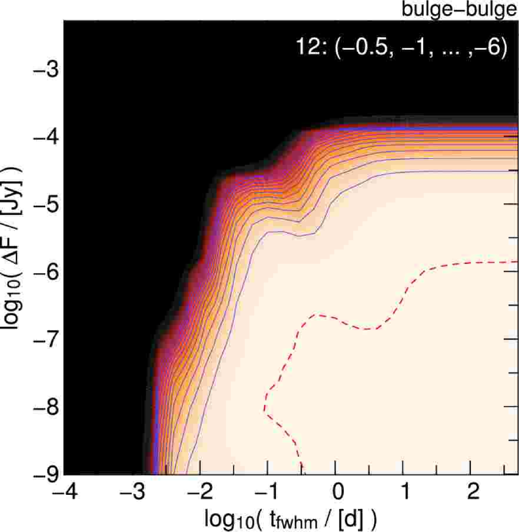
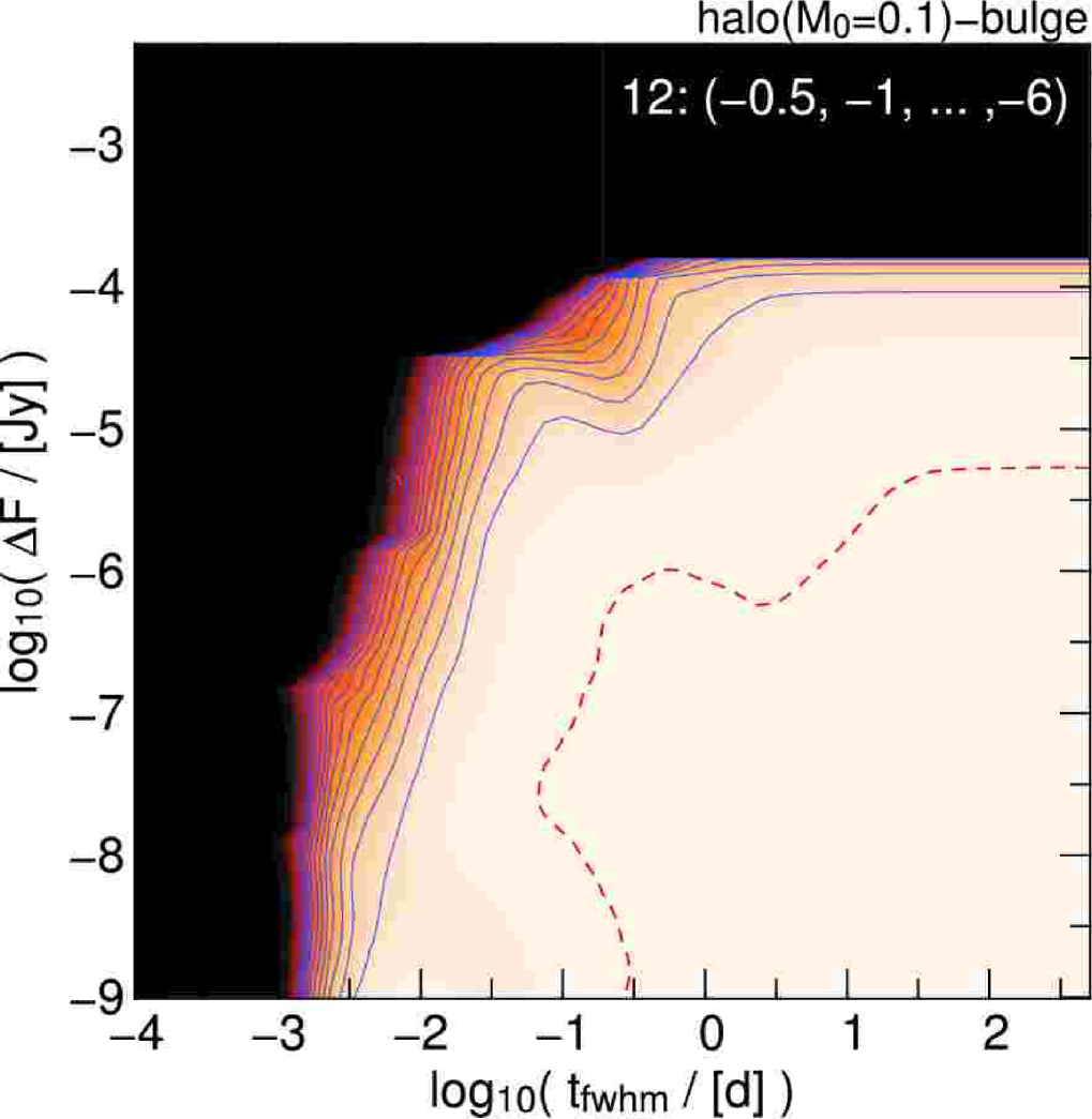
Figure 13.— Ratio of the event rate distribution for extended sources counting events not showing finite source signatures (equation (66) and Figure 11) to the event rate assuming pure point sources (equation (63) and Figure 9), as a function of flux excess and timescale of the events: $\left[d^{2}\Gamma/(d\log{t_{\mathrm{FWHM}}}\,d\log{\Delta_{F}})\right]_{\mathrm{finite\ sources}}\left/\left[d^{2}\Gamma/(d\log{t_{\mathrm{FWHM}}}\,d\log{\Delta_{F}})\right]_{\mathrm{point\ sources}}\right.$ for bulge-bulge (left) and $0.1\,{{M}_{\odot}}$ halo-bulge (right) lensing at $(x,y)=(1\arcmin,0\arcmin)$ in the $\log({\Delta_{F}})$-$\log({t_{\mathrm{FWHM}}})$ plane. The dashed red line marks a ratio of 0.999. The finite source sizes cause a strong suppression of the brightest lensing events relative to the point-source predictions.

In general, the ratio of lensing events with and without finite source signatures is minute for ${t_{\mathrm{FWHM}}}\gtrsim 0.5$d and $\Delta F<10^{-6}$Jy, and raises to about an order of unity for bright lensing events with $\Delta{F_{0}}\approx 1.6\times 10^{-5}$ Jy (corresponding to a magnitude of the excess flux of $m_{R}=20.7\,\mathrm{mag}$) for bulge-bulge-lensing and $\Delta{F_{0}}\approx 5\times 10^{-5}$ ($m_{R}=19.5\,\mathrm{mag}$) for halo-bulge lensing with $0.1\,{{M}_{\odot}}$ lenses. We compare the first column, bulge-bulge lensing, with results for the same lens-source configuration in Figure 9, which had been obtained assuming the full validity of the point-source approximation. The ratio of these contours is shown in Figure 13. The parameter space of interest for current surveys are flux excesses $>10^{-5}\,\mathrm{Jy}$ (excess magnitude of $m_{R}=21.2\,\mathrm{mag}$) and timescales between 1 and 200 days. One can see that the true event rate can differ strongly from that for the point-source approximation depending on the flux excess limit of the survey. The brightest events are preferentially suppressed. This means that taking into account the source sizes is essential for predicting the correct number of lensing events.

Furthermore, one has to be aware that a fair fraction of the brightest lensing events show finite source signatures in their light curves and might be missed when using event filters with a classical lensing event shape in a stringent way. For the detection of finite-source events or even of binary lensing events less stringent thresholds or modified filters are needed, which, however, enhance the risk of a mismatch with variable source detections.

Finally, Figure 12 compares halos with different MACHO masses in its first and second row. An increase in MACHO mass dramatically reduces the event rate and increases the event timescales. This explains the shift in the contours toward longer timescales (compare the change of the ${A_{0}}$-${t_{\mathrm{FWHM}}}$ contours in Fig. 8) and the decrease in the contour levels. For larger MACHO masses, Einstein radii do increase, and one expects finite source effects to become less important: the largest possible flux excess ${\Delta_{F,\mathrm{max}}}$ for the lensing events indeed increases; the size of the shift is as expected, since the maximum flux excess is proportional to the square root of the MACHO mass according to equation (8). The contours in the last row of Figure 12 show MW-halo lensing with $0.1\,{{M}_{\odot}}$ MACHOs. Finite source effects are unimportant. Figures 11 and 12 make it obvious that lensing events above the maximum flux excess predicted for self-lensing would be a clear hint for either massive MACHOs in M31 or MACHOs with unconstrained masses in the Milky Way.

Figure 14 shows the distribution for bulge-bulge lensing splits in color space. The selected color intervals are $0.0<R-I<0.5$, $0.5<R-I<1.0$, and $1.5<R-I<2.0$. In the bluest color interval (first column) we find MS stars close to the MS turnoff as well as SGB, red clump and some RGB stars. The medium red sample contains MS, RGB. and AGB stars, and the reddest sample (last row) contains stars in the RGB and AGB phase and no MS stars. As expected, the timescale of the most likely finite source lensing events changes with color: for the bluest color interval MS stars are responsible for the most likely finite source signature events and the event timescales are very short. The secondary maximum is caused by red clump and SGB stars, which are brighter, need less magnification and therefore have longer event timescales. The color interval of $0.5<R-I<1.0$ contains the central part of the MS, and RGB and AGB stars. The MS stars are fainter (in $R$) and have smaller radii than those in the blue sample, and therefore, the maximally probable event caused by the MS stars is at lower flux excess and timescale than that for the bluer sample. The PMS stars are brighter (which enhances the possibility of longer timescale events) and have larger radii (which leads to stronger peak-flux depression by finite source sizes) than in the bluer sample, and therefore, the events have similar brightness but take longer on average. The reddest color interval, $1.5<R-I<2.0$ contains the reddest PMS stars and no MS stars. These PMS stars are fainter (in $R$) and have larger radii than those contained in the $0.5<R-I<1.0$ sample, and therefore suffer most strongly from finite source effects causing events with even longer timescales than for the bluer PMS stars.

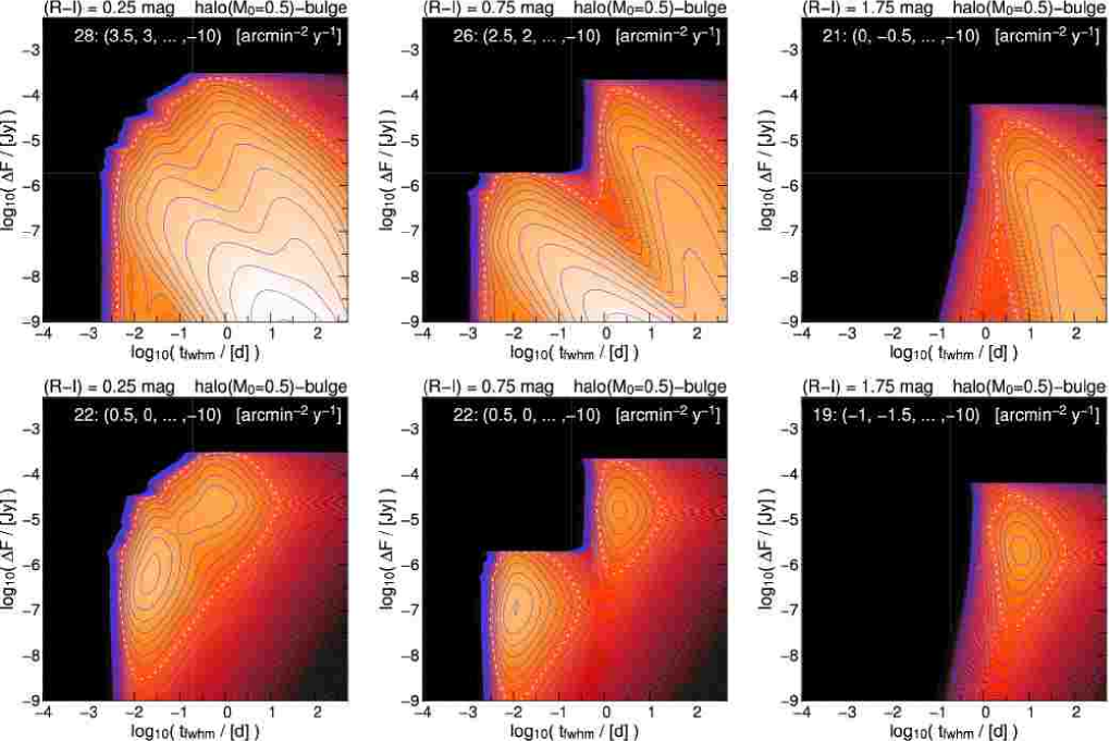
Figure 14.— Distribution $d^{2}\Gamma/(d\log{t_{\mathrm{FWHM}}}\,d\log{\Delta_{F}})$ $[\mathrm{arcmin^{-2}}\,\mathrm{y}^{-1}]$ for $0.5\,{{M}_{\odot}}$ halo-bulge lensing at $(x,y)=(1,0)\,\mathrm{arcmin}$ in the $\log({\Delta_{F}})$-$\log({t_{\mathrm{FWHM}}})$ plane. We show the distribution for bulge sources within different color intervals, $(R-I)\in[0,0.5]\,\mathrm{mag}$ (first column), $(R-I)\in[0.5,1.0]\,\mathrm{mag}$ (second column), and $(R-I)\in[1.5,2.0]\,\mathrm{mag}$ (third column). The upper panels show the distributions for light curves showing no finite source effects, whereas the middle panels show the distributions for light curves with finite source signatures. The lower panels show the sum of both distributions. The contour levels are shown as inserts in each diagram. The dashed line marks the $10^{-3}\,\mathrm{arcmin}^{-2}\,\mathrm{y}^{-1}$ level in each diagram, brighter areas correspond to higher values. See text for more details.

7. Application to Experiments: Total Event Rates and Luminosity Function of Lensed Stars

We now apply our results from §§ 5 and 6 to difference imaging surveys. The goal of this section is to predict realistic event rates that take into account observational constraints (like timescales of events and the signal-to-noise ratios of the light curves, e.g., at maximum). These event rates can be taken for survey preparations or for a first-order comparison of survey results with theoretical models. Exact survey predictions and quantitative comparisons with models can be obtained with numerical simulations of the survey efficiency.

7.1. “Peak-Threshold” for Event Detection

In order to identify a variable object at position $(x,y)$, its excess flux ${\Delta_{F}}$ has to exceed the rms flux $\sigma_{F}(x,y)$ by a certain factor ${Q}$:

$$\begin{array}[]{l}{\Delta_{F}^{\mathrm{min}}}(x,y)={Q}\sigma_{F}(x,y).\end{array}$$ (68)

The parameter $Q$ characterizes the significance of the amplitude of a lensing event, but not of the event itself, since that also depends on the timescale (and the sampling) of the event. We will call events characterized by the signal-to-noise ratio at maximum light “peak-threshold-events” in the following (Baltz & Silk, 2000). Considering only the maximum flux excess of an event (and not its timescale) of course can lead to an over-prediction of lensing events, since events might be too fast to be detected. In addition, long timescale events with low excess flux can have many data points with low significance for the excess flux, which all together make a significant lensing candidate. The detectability of events therefore depends on both its amplitude (flux excess at maximum) and its timescale. This is the reason, why we derived the contribution to the event rate as a function of flux excess and FWHM timescale in § 6.

The flux excess threshold that a source with intrinsic flux ${F_{0}}({\mathcal{M}},{D_{\mathrm{os}}},\mathcal{A})$ must achieve in order to be identified as an event can be translated to thresholds in maximum magnification and relative impact parameter using equations (1) and (7):

$${A_{\mathrm{T}}}(x,y,{F_{0}}({\mathcal{M}},{D_{\mathrm{os}}},\mathcal{A})):={\Delta_{F}^{\mathrm{min}}}(x,y)\,{F_{0}}^{-1}+1\approx{\Delta_{F}^{\mathrm{min}}}(x,y)\,{F_{0}}^{-1},$$ (69)

$${u_{\mathrm{T}}}(x,y,{F_{0}}({\mathcal{M}},{D_{\mathrm{os}}},\mathcal{A})):=\sqrt{\frac{2{A_{\mathrm{T}}}}{\sqrt{{A_{\mathrm{T}}}^{2}-1}}-2}\approx\frac{1}{{A_{\mathrm{T}}}};$$ (70)

in both cases we have also given the high-magnification approximations in the last step.

In contrast to the microlensing regime (where ${u_{\mathrm{T}}}$ is assumed to be constant), ${u_{\mathrm{T}}}$ depends on the local noise value via ${\Delta_{F}^{\mathrm{min}}}(x,y)$ and the luminosity ${\mathcal{M}}$ of the source star being lensed. In Figure 15 we show contours of the minimum magnification required to observe an event at a distance of ${D_{\mathrm{os}}}=770\,\mathrm{kpc}$, source luminosity of ${\mathcal{M}}_{R}=0\,\mathrm{mag}$ and a signal-to-noise threshold of $Q=10$ for a survey like WeCAPP in the $R$ band. Since the M31 surface brightness and thus also the rms photon noise increases toward the center, magnifications of $50$ or larger are needed in the central part. The M31 rms photon noise and rms flux within a PSF in the $R$ band had been estimated using equations (72) and (73) below.

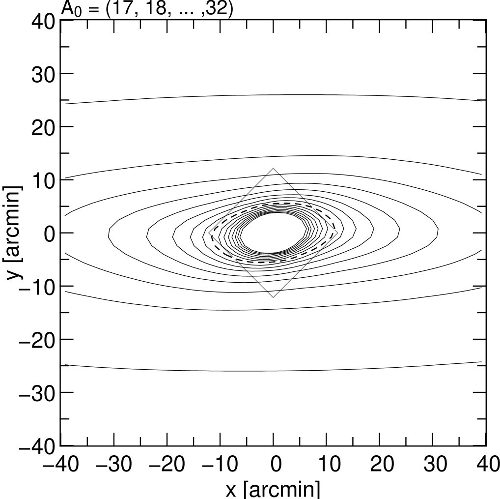
Figure 15.— Contours show the minimum magnifications ${A_{\mathrm{T}}}$ that stars with ${\mathcal{M}}_{R}=0\,\mathrm{mag}$ at a distance of ${D_{\mathrm{os}}}=770\,\mathrm{kpc}$ need to exceed the M31 rms flux by a factor of $Q={\left(\frac{S}{N}\right)}=10$ in the $R$ band, for an experiment (with respect to, e.g., pixel size and seeing) like WeCAPP. The contour levels are ${A_{\mathrm{T}}}=17,18,...,32$. The dashed line marks the ${A_{\mathrm{T}}}=25$ level; the square shows the field observed by WeCAPP given in the intrinsic M31 coordinate system (see Fig. 4).

To obtain an upper limit for the event rate, we assume that all events with flux excesses above the peak-threshold can be identified, irrespective of their timescales. In previous event rate estimates the ${t_{\mathrm{FWHM}}}$ timescales have only been considered correctly in Monte-Carlo simulations. Ignoring the event timescales in analytical estimates the event rate predictions are much more alike the upper limit we present here (eq. [71]). In this case one can simply use the transformation from minimum flux excess at maximum magnification to the threshold relative impact parameter ${u_{\mathrm{T}}}$ in equations (69) and (70) and integrate equation (33) over mass, lens distance, and relative velocities, multiplying it with the relative impact parameter threshold ${u_{\mathrm{T}}}(x,y,{F_{0}}({\mathcal{M}},{D_{\mathrm{os}}},\mathcal{A}))$ and the number density of sources with brightness ${\mathcal{M}}$, $n_{s}(x,y,{D_{\mathrm{os}}})\,\tilde{\Phi}_{s}({\mathcal{M}})$, and finally integrate along the line-of-sight and source luminosity, (§ 4.2):

$$\begin{array}[]{rl}\frac{d^{2}\Gamma_{s,l}}{dx\,dy}=&\int\limits_{0}^{\infty}\int\limits_{0}^{\infty}n_{s}\,\tilde{\Phi}_{s}({\mathcal{M}})\int\limits_{0}^{\infty}\int\limits_{0}^{D_{\mathrm{os}}}\int\limits_{0}^{\infty}\,\int\limits_{0}^{{u_{\mathrm{T}}}(x,y,{F_{0}}({\mathcal{M}},{D_{\mathrm{os}}},\mathcal{A})){R_{\mathrm{E}}}}\frac{d^{4}\Gamma}{d{D_{\mathrm{ol}}}\,d{M}\,d{v_{\mathrm{t}}}\,db}db\,d{v_{\mathrm{t}}}\,d{M}\,d{D_{\mathrm{ol}}}\,d{\mathcal{M}}\,d{D_{\mathrm{os}}}\\ =&\int\limits_{0}^{\infty}\int\limits_{0}^{\infty}n_{s}(x,y,{D_{\mathrm{os}}})\,\tilde{\Phi}_{s}({\mathcal{M}})\,{u_{\mathrm{T}}}(x,y,{F_{0}}({\mathcal{M}},{D_{\mathrm{os}}},\mathcal{A}))\,\Gamma_{1,l}({D_{\mathrm{os}}})\,d{\mathcal{M}}\,d{D_{\mathrm{os}}}.\end{array}$$ (71)

In this equation, the subscript “s” indicates the different stellar populations (bulge, disc) and their sum yields the upper limit for the total event rate. This upper limit for the event rate can therefore be also obtained as a product of the single-star event rate $\Gamma_{1,l}$ (equation (49)), [using ${u_{\mathrm{T}}}(x,y,{F_{0}}({\mathcal{M}},{D_{\mathrm{os}}},\mathcal{A}))$] and the number density of sources with luminosity ${\mathcal{M}}$ on the line of sight. Equation (71) is similar to the equations of Han (1996, eq. (2.5)) and Han & Gould (1996a, eq. (2.2.1)).

Up to now we have not discussed the value of $\sigma_{F}(x,y)$, i.e., the value of the rms flux that appears in the equations for the detection thresholds. This value can in principle be taken from the error propagation in the reduction process. Due to varying observing conditions (seeing, exposure time of the co-added images per night), the errors can differ from day to day by a factor of up to 10; to obtain predictions for the most typical situation, one therefore should use the median error at each image position of a survey to predict the rms flux $\sigma_{F}(x,y)$.

Riffeser et al. (2001) showed that using our reduction pipeline (that propagates true errors through all reduction steps) errors in the light curves are dominated by the photon-noise contribution of the background light. Therefore the typical error can be estimated from the surface brightness profile ${\mu}(x,y)$ of M31 and the typical, i.e., median, observing conditions of the survey. Using analytically predicted rms-values, one can study the impact of the observing conditions on event rates and optimize survey strategies.

To measure the variability of objects one has to perform (psf-)photometry defining the angular area of the psf $\Omega_{\mathrm{psf}}:=\pi\,\theta_{\mathrm{psf}}^{2}/\ln{4}$ and the FWHM of the psf $\theta_{\mathrm{psf}}$. For a given experimental setup the rms photon noise $\sigma_{\mathrm{photon}}(x,y)$ within an area $\Omega_{\mathrm{psf}}\,[\mathrm{arcsec}^{2}]$ at a position $(x,y)$ is

$$\sigma_{\mathrm{photon}}(x,y):=\left[\left(10^{-0.4({\mu}(x,y)+\kappa\,\mathrm{AM})}+10^{-0.4\,{\mu}_{\mathrm{sky}}}\right)10^{-0.4(-\mathrm{ZP})}\,t_{\mathrm{exp}}\,\Omega_{\mathrm{psf}}\right]^{1/2},$$ (72)

where ${\mu}_{\mathrm{sky}}$ [mag arcsec^-2] is the sky surface brightness, $t_{\mathrm{exp}}$ is the exposure time in seconds, $\mathrm{AM}$ is the air mass of the observation, $\mathrm{ZP}$ is the photometric zero point of the telescope camera configuration in photons per second and $\kappa$ is the atmospheric extinction for the observing site.

The rms photon noise can be translated to the rms flux (in Jy) using the flux of Vega, ${F_{\mathrm{Vega}}}$, and its magnitude $m_{\mathrm{Vega}}=0$:

$$\sigma_{F}(x,y):=\frac{{F_{\mathrm{Vega}}}}{t_{\mathrm{exp}}\,10^{-0.4(m_{\mathrm{Vega}}+\kappa\,\mathrm{AM}-\mathrm{ZP})}}\;\sigma_{\rm photon}={F_{\mathrm{Vega}}}\left[\left(10^{-0.4({\mu}(x,y)+\kappa\,\mathrm{AM})}+10^{-0.4\,{\mu}_{\mathrm{sky}}}\right)10^{0.8\,\kappa\,\mathrm{AM}}\,10^{-0.4\,\mathrm{ZP}}\,\frac{\Omega_{\mathrm{psf}}}{t_{\mathrm{exp}}}\right]^{1/2}.$$ (73)

The last equation shows that the rms flux within an aperture is proportional to $t_{\mathrm{exp}}^{-1/2}$, making the signal-to-noise $Q$ proportional to $t_{\mathrm{exp}}^{1/2}$, as expected for background noise-limited photometry of point-like objects.

The extincted surface brightness profile ${\mu}(x,y)$ in Eqs. 72 and 73 can be taken either from very high signal-to-noise measurements of M31 or from analytical models that are constructed to match the observed SFB-profile and dynamics of M31. In the latter case, the extincted surface brightness ${\mu}(x,y)$-model combines the luminous matter density $\rho_{s}(x,y,{D_{\mathrm{os}}})$ with the mass-to-light ratio for each source components ($s$=bulge,disk) and accounts for Galactic and intrinsic extinction $\mathcal{A}(x,y,{D_{\mathrm{os}}})$ along the line-of-sight:

$$\begin{array}[]{l}{\mu}(x,y)=-2.5\log\left({F_{\mathrm{Vega}}}^{-1}\sum\limits_{s}\,\int\limits_{0}^{\infty}10^{-0.4\,\mathcal{A}(x,y,{D_{\mathrm{os}}})}\,\frac{\rho_{s}(x,y,{D_{\mathrm{os}}})}{{\left(\frac{M}{L}\right)}_{s}\,\frac{{{M}_{\odot}}}{{{\mathcal{F}}_{\odot}}}}\left(\frac{10\,\mathrm{pc}}{{D_{\mathrm{os}}}}\right)^{2}\left(\frac{2\pi}{360\times 3600}\right)^{2}{D_{\mathrm{os}}}^{2}\,d{D_{\mathrm{os}}}\right)\end{array},$$ (74)

where the units are $\mathrm{mag}\,\mathrm{arcsec}^{-2}$.

7.2. “Event-Threshold” for Event Detection

Gould & Han (Gould, 1996b; Han, 1996; Han & Gould, 1996a) introduced an “event threshold”, where the detectability of events depends on the total excess light of the light curves. They obtained an implicit equation for the threshold ${u_{\mathrm{T}}}$ of the relative impact parameter,

$$\frac{\zeta({u_{\mathrm{T}}})}{{u_{\mathrm{T}}}}=\frac{t_{\mathrm{cyc}}\,\sigma_{F}(x,y)^{2}}{\overline{{t_{\mathrm{E}}}}(x,y,{D_{\mathrm{os}}})\,\pi{F_{0}}^{2}}{Q_{\mathrm{event}}}^{2},$$ (75)

where $\sigma_{F}(x,y)$ is the rms flux at that position and $\overline{{t_{\mathrm{E}}}}(x,y,{D_{\mathrm{os}}})$ is the mean Einstein time of the events (equation (54)); $\zeta$ is defined by

$$\zeta({u_{0}}):=\frac{\int\left[A(t)-1\right]^{2}\,dt}{\int\left[(t/{t_{\mathrm{E}}})^{2}+{u_{0}}^{2}\right]^{-1}\,dt},$$

${F_{0}}({\mathcal{M}},{D_{\mathrm{os}}},\mathcal{A})$ is the unlensed source flux and $t_{\mathrm{cyc}}$ is the (equidistant) difference between observations.

This equation assumes equidistant sampling of the light curves and is therefore most readily applied to space-based experiments. In addition, it takes into account the mean Einstein timescale of events only, although the relative impact parameter threshold depends on the individual timescale of the event. For realistic event rate estimates, however, one has to to take into account the timescale distributions, as well.

One can in fact obtain an analog relation for flux excess ${\Delta_{F}}$ and ${t_{\mathrm{FWHM}}}$ timescale of the events (i.e., the actual observables),

$${\Delta_{F}^{\mathrm{min}}}^{2}\,\tilde{\zeta}{\left(\frac{{F_{0}}}{{\Delta_{F}^{\mathrm{min}}}},{t_{\mathrm{FWHM}}}\right)}=\frac{\sqrt{12}\,t_{\mathrm{cyc}}\,\sigma_{F}(x,y)^{2}}{\pi\,{t_{\mathrm{FWHM}}}}{Q_{\mathrm{event}}}^{2},$$ (76)

with

$$\tilde{\zeta}({A_{0}}-1,{t_{\mathrm{FWHM}}}):=\frac{\int\left[A(t)-1\right]^{2}\,dt}{\int({A_{0}}-1)\left[12(t/{t_{\mathrm{FWHM}}})^{2}+1\right]^{-1}\,dt}.$$

Equation (76) can be numerically inverted to obtain the peak flux threshold ${\Delta_{F}^{\mathrm{min}}}({t_{\mathrm{FWHM}}},x,y,{\mathcal{M}})$ as a function of the event timescale. Therefore, it is obvious that the peak threshold and event threshold criteria are related assuming equidistant sampling and that the event threshold criterion is a special case of the peak threshold plus a ${t_{\mathrm{FWHM}}}$ threshold criterion, which is evaluated in equation (77) (see § 7.3).

7.3. Total Event Rate with Excess Flux Threshold ${\Delta_{F}^{\mathrm{min}}}$ and Timescale ${t_{\mathrm{FWHM}}^{\mathrm{min}}}$ Threshold

The upper limit derived in § 7.1 still includes numerous events that cannot be detected in finite time resolution experiments. At this point, where not only must the flux excess (maximum magnification or relative impact parameter) of the event be considered, but also the timescale of the event, the transformation of the event rate from the “theoretical quantities” to the “observational quantities” in § 6 becomes most relevant. Using equation (63) we can simply integrate from the lower limits ${\Delta_{F}^{\mathrm{min}}}$ and ${t_{\mathrm{FWHM}}^{\mathrm{min}}}$ to infinity (or any other value specified by the experiment):

$$\frac{d^{2}\Gamma_{l,s}}{dx\,dy}:=\int\limits_{{t_{\mathrm{FWHM}}^{\mathrm{min}}}(x,y)}^{\infty}\,\int\limits_{{\Delta_{F}^{\mathrm{min}}}({t_{\mathrm{FWHM}}},x,y)}^{\infty}\frac{d^{4}\Gamma_{s,l}}{dx\,dy\,d{t_{\mathrm{FWHM}}}\,d{\Delta_{F}}}\,d{\Delta_{F}}\,d{t_{\mathrm{FWHM}}}$$ (77)

with

$$\frac{d^{4}\Gamma_{s,l}}{dx\,dy\,d{t_{\mathrm{FWHM}}}\,d{\Delta_{F}}}:=\int\int\frac{d^{6}\Gamma_{s,l}}{dx\,dy\,d{t_{\mathrm{FWHM}}}\,d{\Delta_{F}}\,d{M}\,d{\mathcal{M}}}\,d{M}\,d{\mathcal{M}}.$$

The thresholds ${t_{\mathrm{FWHM}}^{\mathrm{min}}}(x,y)$ and ${\Delta_{F}^{\mathrm{min}}}({t_{\mathrm{FWHM}}},x,y)$ (see eqs. [68] and [76]) are set by the experiment and the detection process.

Table 1Observational setups for the WeCAPP survey and a potential experiment using the ACS on board of HST

Parameter	WeCAPP	HST with ACS WFC
$t_{\mathrm{exp}}$ (s)	500	1000
$l_{\mathrm{pixel}}$ (arcsec)	0.5	0.049
Field of view (pixels)	$2048\times 2048$	$4096\times 4096$
Field of view (arcmin)	$17.2\times 17.2$	$3.37\times 3.37$
Filter	Johnson R	F625W
$\mathrm{ZP}$ (mag)	23.68	25.73 (De Marchi et al. (2004), Table 3)
Average $\mathrm{sky}$	20.0	22.5
FWHM of the psf $\theta_{\mathrm{psf}}$ (arcsec)	1.5	0.12 (Krist (2003), p. 13)
$\Omega_{\mathrm{psf}}$ (arcsec2)	5.1	0.033
AM	1.0	0
Atmospheric extinction $\kappa_{R}$	0.1	0
${\Delta t}$ (days)	200	30
${t_{\mathrm{FWHM}}^{\mathrm{min}}}$ (days)	1	1
${t_{\mathrm{FWHM}}^{\mathrm{max}}}$ (days)	200	20
inner saturation radius (arcsec)	20	0
CCD orientation angle (deg)	45	0

For the WeCAPP experiment (see Table 1) toward M31 it turned out that the efficiency can easily be evaluated using Monte-Carlo simulations. As in the WeCAPP experiment errors are propagated through all reduction steps (Riffeser et al., 2001); the final errors in the light curve $\sigma(x,y,t_{i})$ include the full reduction procedure. For a simple set of detection limits, i.e., ${\Delta_{F}^{\mathrm{min}}}\sim\sigma$ and ${t_{\mathrm{FWHM}}^{\mathrm{min}}}={\mathrm{const}}$, the efficiency ${\epsilon}(x,y,{t_{\mathrm{FWHM}}},{\Delta_{F}})$ for a survey can easily be evaluated as a function of the directly observable parameters $x$, $y$, ${t_{\mathrm{FWHM}}}$, and ${\Delta_{F}}$ (in contrast to the variables ${t_{\mathrm{E}}}$ and ${A_{0}}$). This and more sophisticated thresholds (as used in Alcock et al. (2001b)) and efficiency simulations for WeCAPP we will present in a forthcoming paper.

Using this efficiency we can generalize equation (77) to

$$\frac{d^{2}\Gamma_{l,s}}{dx\,dy}:=\int\int\frac{d^{4}\Gamma_{s,l}}{dx\,dy\,d{t_{\mathrm{FWHM}}}\,d{\Delta_{F}}}\,{\epsilon}(x,y,{\Delta_{F}},{t_{\mathrm{FWHM}}})\,d{\Delta_{F}}\,d{t_{\mathrm{FWHM}}}.$$ (78)

As the total event rate depends on the model parameters of the luminous and dark component, precise measurements of the event numbers and event rate’s spatial variation can in principle constrain the source and lens densities [$\rho_{l}(x,y,{D_{\mathrm{ol}}})$, $n_{s}(x,y,{D_{\mathrm{os}}})$], the lens mass functions [$\xi_{l}({M})$], the distribution of the transversal velocities [${p_{v_{\mathrm{t}}}}({v_{\mathrm{t}}},v_{0}(x,y,{D_{\mathrm{ol}}},{D_{\mathrm{os}}}))$], the luminosity function of the sources [$\tilde{\Phi}_{s}({\mathcal{M}})$ or ${p_{\mathrm{cmd}}}_{s}({\mathcal{M}},{\mathcal{C}})$], and finally the MACHO fraction in the halo. There are, of course other valuable parameters, like event duration, flux excess distribution, color of the lensed stars, and finite source effects, which make the lensing analysis much more powerful than the pure counting of events.

Table 2 summarizes the event rate predictions for the WeCAPP experiment toward the bulge of M31, using different realistic thresholds for the signal-to-noise threshold necessary to derive “secure” events, and for ${t_{\mathrm{FWHM}}^{\mathrm{min}}}$. These numbers do not take into account that events cannot be observed when M31 is not visible (one-third of the year), that in the remaining time some – in particular short-term events – escape detections because of observing gaps, and that some of the area is not accessible for identification of lensing events due to intrinsically variable objects. We calculated the predictions for signal-to-noise thresholds of $Q=10$ and $Q=6$; these thresholds correspond to flux excess thresholds of $6.2\times 10^{-6}\,\mathrm{Jy}$ (Q=10) and $3.7\times 10^{-6}\,\mathrm{Jy}$ (Q=6) in the edges and $2.4\times 10^{-5}\,\mathrm{Jy}$ (Q=10) and $1.5\times 10^{-5}\,\mathrm{Jy}$ (Q=6) 20″ off center (outside saturation) of the WeCAPP field. The $Q>10$ events are events like those published in the past (e.g., WeCAPP-GL1 and WeCAPP-GL2 have values of $Q\approx 85$ and $Q\approx 16$), whereas $Q=6$ should be more similar to the medium bright event candidates of MEGA. For the $Q=10$ cases we have separated events that do not show finite source effects in the light curves (“without fs”) from those which show finite source effects (“with fs”). Finite source events are relatively more important for high signal-to-noise, short timescale self-lensing events. In most current pixel-lensing surveys, light curves with finite source effects are not specially searched for and may preferentially get lost in the detection process, unless one allows for a less good fit for bright events.

For the $Q=6$, ${t_{\mathrm{FWHM}}}=2\,\mathrm{days}$ case we split the predictions into the near and far side of M31. Within our field, the predicted halo-bulge asymmetry is small, but the bulge-disk and halo-disk asymmetry are on a noticeable level. (Note that the disk-bulge lensing does show the reversed asymmetry). It has been pointed out in the past (An et al. (2004)) that dust lanes in the M31 disk are an additional source of asymmetry; this is obvious if one considers the spatial distributions of variables found in pixel-lensing experiments (see An et al. (2004), Ansari et al. (2004) and Fliri et al. (2006)). These can, however, be taken to quantitatively account for extinction, in addition to extinction maps. The values given in our table do not account for the small spatial dependence of extinction and thus place lower limits to the observed far-near asymmetry of the individual lens-source configuration.

The comparison for different timescale thresholds (cases III, IV, and V) shows that (except high mass halo lensing) the majority of events has timescales smaller than 10 days. A clustering of event candidates with short and long timescales as de Jong et al. (2004) observed for the MEGA analysis of the POINT AGAPE survey (they obtained 6 candidates with timescales smaller than 10 days and 8 candidates with timescales larger than $20\,\mathrm{d}$) can be hardly explained for the WeCAPP field. This is because, even for supermassive MACHOs, one would expect roughly as many events between 2 and 20 days than above 20 days (compare case III and case V in Table 2). de Jong et al. (2004) argue that their long-term events arise in the outskirts of M31, where the photon noise is smaller, and could be understood from selection effects. This would still lack to explain the bimodality of timescales. At the moment it is not excluded that these long-term event candidates are still misidentified variable objects. In the last line we add the analogous numbers for halo lensing resulting from Milky Way halo lenses of 0.1 ${{M}_{\odot}}$. The number of MACHO events caused by the MW MACHOs should be roughly one-third of that caused by M31 MACHOs.

Table 2Total event rate $\Gamma_{s,l}$ $[\,\mathrm{y}^{-1}]$ for the WeCAPP experiment for self-lensing and halo-lensing

Model	I			II			III						IV			V
							Near Side			Far Side
b-b	1.2	+	1.9	0.57	+	0.68	1.4	+	0.98	1.4	+	0.99	0.16	+	0.046	0.026	+	0.0062
h0.1-b	8.2	+	5.4	4	+	1.7	6.3	+	1.6	7.1	+	1.9	0.92	+	0.071	0.16	+	0.0094
h0.5-b	7.4	+	2.7	4.4	+	1	5.5	+	0.72	6.3	+	0.82	1.8	+	0.051	0.47	+	0.0074
h1000-b	0.7	+	0.0013	0.61	+	0.0011	0.51	+	0.00051	0.59	+	0.00056	0.75	+	0.00025	0.6	+	$5\times 10^{-5}$
d-b	0.57	+	0.34	0.26	+	0.098	0.89	+	0.16	0.087	+	0.026	0.057	+	0.0029	0.0072	+	0.00031
hMW0.1-b	3.9	+	0.0046	1.9	+	0.0019	2.7	+	0.001	2.7	+	0.001	0.47	+	$4\times 10^{-5}$	0.088	+	$5\times 10^{-6}$
hMW0.5-b	2.4	+	0.0009	1.5	+	0.0002	1.8	+	0.0001	1.8	+	0.0001	0.76	+	$2\times 10^{-6}$	0.23	+	$3\times 10^{-7}$
b-d	2.3	+	1.6	1.4	+	0.77	0.43	+	0.22	3.8	+	1.3	0.43	+	0.049	0.082	+	0.0055
h0.1-d	11	+	4.3	6.6	+	2	4.9	+	0.72	12	+	2	2.1	+	0.1	0.5	+	0.014
h0.5-d	8.6	+	1.2	5.8	+	0.65	3.6	+	0.21	9.5	+	0.55	3.1	+	0.069	1	+	0.011
h1000-d	0.61	+	0.00015	0.56	+	0.00014	0.26	+	$5\times 10^{-5}$	0.7	+	$9\times 10^{-5}$	0.7	+	$8\times 10^{-5}$	0.55	+	$2\times 10^{-5}$
d-d	0.2	+	0.13	0.14	+	0.075	0.2	+	0.056	0.19	+	0.056	0.095	+	0.018	0.036	+	0.0055
hMW0.1-d	3.1	+	0.0019	2	+	0.00049	2.2	+	0.00025	2.2	+	0.00024	0.95	+	$6\times 10^{-6}$	0.3	+	$7\times 10^{-7}$
hMW0.5-d	1.9	+	0.00022	1.4	+	0.00013	1.4	+	$7\times 10^{-5}$	1.4	+	$7\times 10^{-5}$	0.97	+	$4\times 10^{-6}$	0.43	+	$5\times 10^{-7}$

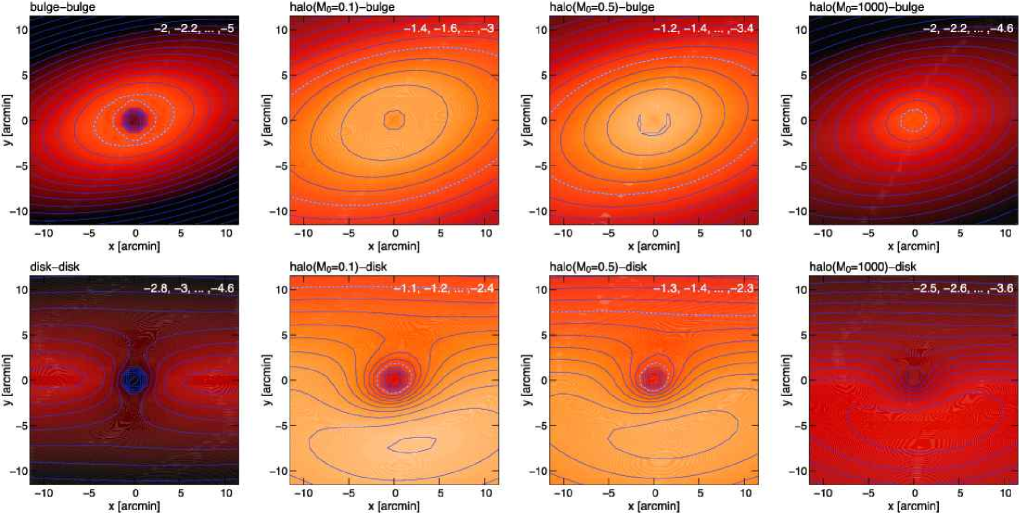
Figure 16.— Event rate maps in logarithmic units (in units of events $\mathrm{yr}{{}^{-}1}\,\mathrm{arcmin}^{-2}$) for the WeCAPP survey for ${Q}=10$ and ${t_{\mathrm{FWHM}}^{\mathrm{min}}}=1\,\mathrm{d}$ (column labeled ”I” in Table 2). Coordinates are given in the intrinsic M31 coordinate system (see Figure 4). The contour levels are shown in inserts in the upper right corners of each diagram. The dashed line marks the $0.01\,\mathrm{ev}\,\mathrm{y}^{-1}\,\mathrm{arcmin}^{-2}$ level in each diagram. The event rate decreases near the center of M31 due to higher noise combined with finite source effects. Note that the maximum lensing (maximum optical depth) region defined by Crotts (1992) and Tomaney & Crotts (1996) is predicted at about $1.5\,\mathrm{kpc}$ ($7.5\arcmin$) from the nucleus for a simple halo model. For the calculations we have taken into account the finite stellar source sizes; the numbers shown, however, include only those among all events that do not show finite source signatures in their light curves, i.e., those which are usually searched for in lensing experiments.

Figure 16 shows the predictions for the spatial distribution of the lensing events for the WeCAPP survey, evaluated for the $Q=10$ and ${t_{\mathrm{FWHM}}}=1\,\mathrm{day}$ thresholds (column labeled “I” in Table 2). One can see that the event rate density becomes maximal close to the M31 center for bulge-bulge and halo-bulge lensing configurations. That seems counterintuitive to the results about the lensing optical depth and single-star event rate in Figures 4 and 5, where the maximum is attained on the M31 far side, significantly offset from the center. This difference is due to the density of source stars, which rises toward the center much more than the single-star event rate and the detectability of the events drops. As can also be seen in Table 2, a far to near side asymmetry (lower and upper part in the figure) is not present for bulge-bulge lensing, is modest for halo-bulge lensing, and is stronger for the disk-bulge lensing. This is because the disk effectively cuts the bulge in one part in front and the other behind the disk, and only the stars in the second part can contribute to disk-bulge lensing. The bulge-disk self-lensing shows the opposite far to near side asymmetry and attains its maximum event rate per area in the far side of the disk. The same is true for the halo-disk lensing (main maximum on far side of disk), which shows a secondary maximum close to the M31 center caused by the increase of the disk-star density. The disk-disk lensing event rate per area is symmetric with respect to the near and far side of the disk. The fact that the maximum for bulge-bulge and disk-disk lensing is not located exactly at the M31 center is caused by the increased photon noise combined with finite-source effects.

The total self-lensing (disk-bulge + bulge-disk + bulge-bulge + disk-disk) shows an asymmetry arising from the different luminosity functions and mass functions of the bulge and disk population which leads to different event characteristics for disk-bulge and bulge-disk lensing. Therefore, lens and source populations cannot easily be exchanged. The fact that the near side is closer to us – lensing strength and apparent magnitude of sources change by a few percent – than the far side of M31 plays a minor role for the asymmetry of self-lensing event rates.

The last figure (Fig. 17) in this section shows the total event rates $\Gamma_{l,s}({t_{\mathrm{FWHM}}^{\mathrm{min}}},Q)=\int\int\frac{d^{2}\Gamma_{l,s}}{dx\,dy}\,dx\,dy$ in the WeCAPP field depending on the peak flux threshold and the timescale threshold of the survey. We have taken into account the finite source sizes but show only the rate for those events that do not show any finite source signature in their light curves.

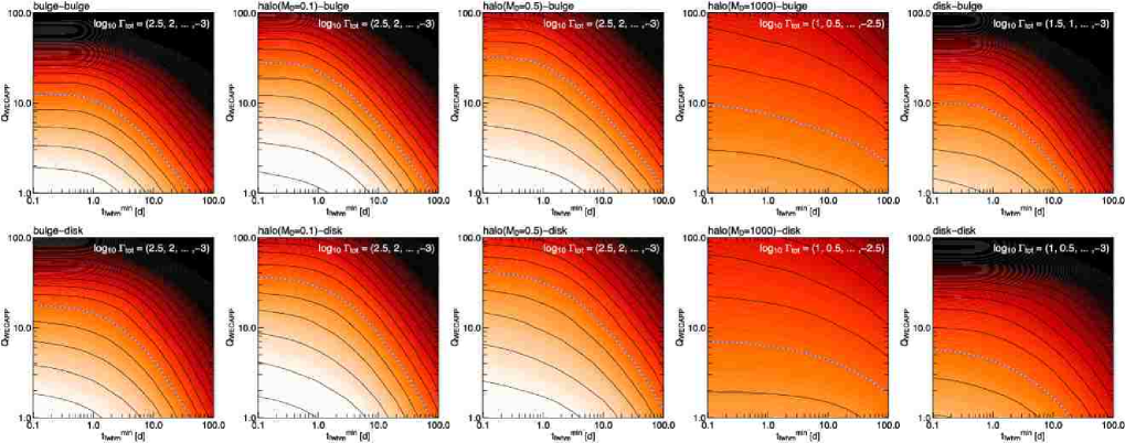
Figure 17.— Contours of the logarithm of the lensing event rate per year within the $17.2\arcmin\times 17.2\arcmin$ WeCAPP field as a function of the signal-to-noise threshold $Q$ for the peak-flux excess and as a function of the timescale threshold of the events. For these numbers, eq. (77) was integrated over the WeCAPP field, and the noise was estimated for the WeCAPP survey (characterized by Table 1). We show results for different lens-source configurations, from left to right: bulge-bulge self-lensing, halo-bulge lensing with $0.1\,{{M}_{\odot}}$ lenses, halo-bulge lensing with $0.5\,{{M}_{\odot}}$ lenses, and disk-bulge self-lensing. The blue dashed line marks the 1 event per year level. For the calculations we have taken into account the finite stellar source sizes; the numbers shown, however, include only those among all events that do not show finite source signatures in their light curves, i.e., those which are usually searched for in lensing experiments. For signal-to-noise ratios of $Q>10$, the rates for events with finite source effects can be of the same order as the rates for events with point-source light curves. For lower signal-to-noise ratios, events with finite source effects become much less important.

For high signal-to-noise events (e.g., $Q=20$), all configurations do show more or less flat contours in the ${t_{\mathrm{FWHM}}}$ direction for ${t_{\mathrm{FWHM}}}$ values between $0.1$ and $1$ days. This indicates that there are relatively few very high signal-to-noise events with timescales around $0.1$ days compared to events with timescales of about $1$ day. That this is true is confirmed by Figures 11 and 12, which show that the highest signal-to-noise and thus highest flux excess events occur with timescales between $0.6$ and a few days and that events with timescales of about $0.1$ days are significantly fainter. Only for smaller flux excesses, the events with timescales of $0.1$ days can be as common as events with timescales of a couple of days. This implies that if one can measure only lensing events that have a $(S/N)$ ratio of $Q\geq 10$ in the WeCAPP setup, one cannot greatly increase the number of observed events by increasing the sampling (the largest increase for sampling below 1 day would occur for halo-disk lensing). The detectability of events with timescales of hours can therefore be increased effectively only (in the central M31 field), if the noise level of the observations is lowered. It can also be seen in all panels of Figure 17 that one expects the number of events to decrease strongly for ${t_{\mathrm{FWHM}}}$-thresholds larger than several days. The quantitative differences in the different lensing configurations in the subpanels of Figure 17 can be easily understood (by combining the dependence of the event rate on event timescale and magnification with the luminosity function of source stars, and accounting for the difference in the importance of finite source effects) and are discussed for the $0.1\,{{M}_{\odot}}$ MACHO bulge and the $0.5\,{{M}_{\odot}}$ MACHO bulge lensing case. Table 2 already suggests that these two lensing configurations are very similar for the event numbers that do not show finite source signatures (the $0.1\,{{M}_{\odot}}$ MACHOs do cause more high signal-to-noise finite source events). One expects that the increase of the MACHO mass decreases the total event rate per line-of-sight (fewer lenses) but also increases the events’ timescales. On the basis of the event rate per timescale and event magnification (Figure 8) one would therefore expect longer timescales but fewer events for the stellar mass MACHO case. This simple picture is altered by the finite source effects, which limit the maximal flux excess and thus signal-to-noise of an event. The question, whether one expects more events for brown dwarf or stellar mass MACHOs depends therefore on the combination of signal-to-noise threshold and timescale threshold.

The predicted event rates rise strongly for lower $Q$ thresholds. This means that if one lowers the (S/N) threshold – or equivalently increases the signal or decreases the noise level by changing the experiment – one could dramatically increase the event rates. This can be achieved by an increase of telescope area and integration time, but much better with a decrease of the PSF of the experiment. This makes the space experiments most promising. In addition, the comparison of the subpanels in Figure 17 shows that the bulge-bulge lensing rate will profit much stronger from a decrease of the noise than any other lensing configuration.

Assume that the center of M31 is monitored with the ACS on 30 consecutive days, with three 6 minute exposures in the F625W band and two 6 minute exposures in the F555W band, which would need one orbit per day altogether (see more details in Table 1). Assume furthermore that the background light has the level of the smoothed M31 SFB isophotes (in reality a fraction of the brightest stars gets resolved lowering the background light in between the resolved objects). Using that background level, we predict the event rates with timescales between 1 and 20 days for bulge-bulge self-lensing and halo-bulge lensing in Table 3. If one assumes a halo fraction of about 25% then the halo-lensing events do not contribute more than 10% relative to the bulge-bulge lensing rate.

Table 3Total event rates $\Gamma_{s,l}$ $[\,\mathrm{y^{-1}}]$ for a 30 day, 1-orbit-per day HST ACS experiment (see Table 1)

Model	Without fs	With fs
b - b	1350	100
h0.1 - b	620	10

Current measurements of extragalactic mass functions reach masses down to 0.6 solar masses (for the LMC Gouliermis et al. (2005)). Microlensing allows a measurement of the low-mass end of the stellar mass function, while not relying on the luminosity of those low-mass stars. The mass of these stars becomes visible by their lensing effect on (in general) brighter stars. Therefore, M31 bulge-lensing combined with space observations makes it possible to test an extragalactic mass function well below $0.5\,{{M}_{\odot}}$.

7.4. The Luminosity Function Sensitivity

Whereas the probability for a star to be lensed does not depend on its luminosity, the probability that the event can be detected strongly depends on the luminosity of the source star. This implies that the luminosity function of the source stars of lensing events is biased toward high-luminosity stars. The selection probability of a star with luminosity ${\mathcal{M}}$, which we call “luminosity function sensitivity”, is obtained with equation (63) as

$$\frac{1}{\tilde{\Phi}_{s}({\mathcal{M}})}\frac{d^{3}\Gamma_{s,l}}{dx\,dy\,d{\mathcal{M}}}=\int\limits_{t_{\mathrm{FWHM}}^{\mathrm{min}}}^{\infty}\int\limits_{\Delta_{F}^{\mathrm{min}}}^{\infty}\frac{2}{{t_{\mathrm{FWHM}}}^{3}}\int\limits_{0}^{\infty}\,\xi_{l}\int\limits_{0}^{\infty}n_{s}\,\frac{\Psi}{{F_{0}}}\int\limits_{0}^{D_{\mathrm{os}}}\rho_{l}\,{R_{\mathrm{E}}}^{3}\,{p_{v_{\mathrm{t}}}}{\left(\frac{{R_{\mathrm{E}}}\Upsilon}{{t_{\mathrm{FWHM}}}},v_{0}\right)}\,d{D_{\mathrm{ol}}}\,d{D_{\mathrm{os}}}\,d{M}\,d{\Delta_{F}}\,d{t_{\mathrm{FWHM}}},$$ (79)

with the parameters and relations used for $\tilde{\Phi}_{s}{\left({\mathcal{M}}\right)}$, $\xi_{l}({M})$, $n_{s}(x,y,{D_{\mathrm{os}}})$, $\rho_{l}(x,y,{D_{\mathrm{ol}}})$, ${R_{\mathrm{E}}}({D_{\mathrm{ol}}},{M},{D_{\mathrm{os}}})$, ${F_{0}}({\mathcal{M}},{D_{\mathrm{os}}})$, $\Psi({A_{0}}({F_{0}},{\Delta_{F}}))$, $\Upsilon({A_{0}}({F_{0}},{\Delta_{F}}))$. The luminosity function sensitivity gives the event rate per area per source star luminosity bin, normalized by the luminosity function $\tilde{\Phi}_{s}({\mathcal{M}})$. In Figure 18 we show results for the luminosity function sensitivity using equation (79) for several minimal detectable timescales ${t_{\mathrm{FWHM}}^{\mathrm{min}}}$ (0, 0.01, 0.1, 1, and 10 days) using the configuration of the WeCAPP and ACS experiments and the model of M31 presented in § B.

Figure 18 shows that the sensitivity strongly increases with decreasing timescale thresholds. Applying no ${t_{\mathrm{FWHM}}}$ threshold for the total event rate (equivalent to evaluating equation (71)) overestimates the luminosity sensitivity for faint MS stars. In consequence, the total event rate is overestimated as well. Accounting for the timescale thresholds for microlensing surveys (i.e., using equation (77) for the total event rate) suppresses the contribution of faint stars and yields a much more realistic estimate of the total event rate. In Figure 18 (right) we show the luminosity function of the sources for lensing events, which is obtained as the product of the luminosity function sensitivity and the luminosity function $\tilde{\Phi}_{s}({\mathcal{M}})$. The results differ for an experiment like WeCAPP and an experiment with small PSF noise like the suggested ACS imaging campaign.

An experiment like WeCAPP induces a cutoff of ${\mathcal{M}}_{R}\approx 6\,\mathrm{mag}$ in the luminosity of the lensed stars, because one would need magnifications larger than the finite source size magnification limit to obtain an observable flux excess for source luminosities below that value. This cutoff is valid for all lens-source configurations within M31, with the exception of supermassive M31 MACHOs, and it does not hold for lensing by MW MACHOs. With an ACS experiment, the minimum measurable flux excess is much smaller than for WeCAPP, and therefore even the faintest MS stars can act as sources for detectable lensing events (no cutoff in the luminosity function of lensed stars). For events with timescales above 1 day, the luminosity function of lensed stars becomes almost flat for magnitudes brighter than ${\mathcal{M}}_{R}\approx 4\,\mathrm{mag}$ (green curve).

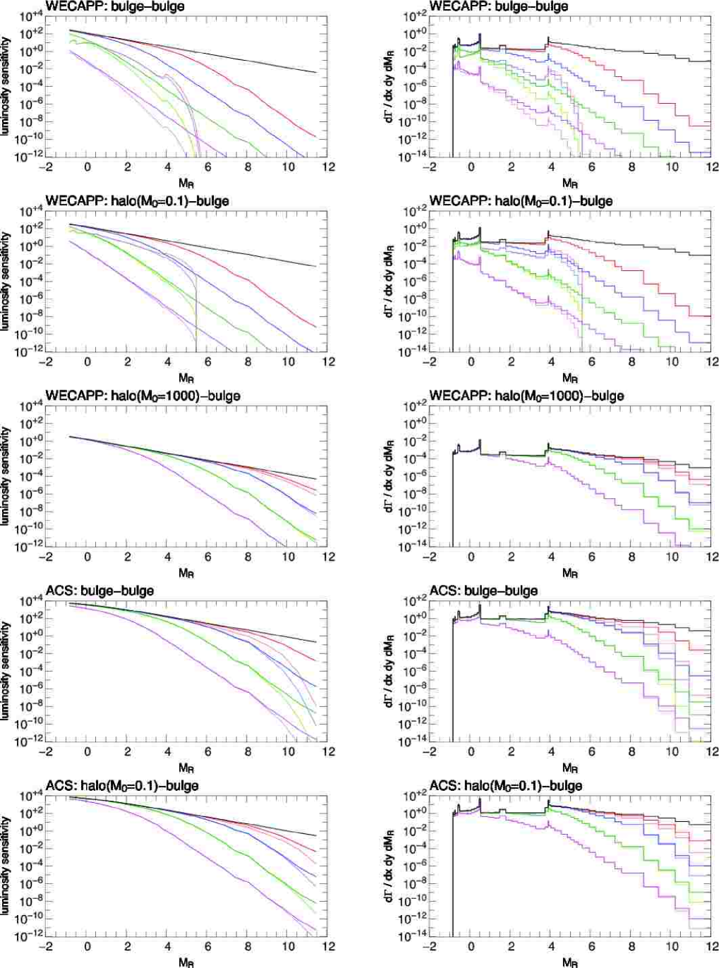
Figure 18.— Left panel: Luminosity function sensitivity (eq. [79]) $[\mathrm{arcmin}^{-2}\,\mathrm{y}^{-1}]$ for bulge-bulge, $0.1\,{{M}_{\odot}}$ halo-bulge, $1000\,{{M}_{\odot}}$ halo-bulge lensing in the WeCAPP and ACS experiment (see § B) with ${Q}=12$ at $(x,y)=(1,0)\,\mathrm{kpc}$ (corresponding ${\Delta_{F}^{\mathrm{min}}}=1.7\times 10^{-5}\,\mathrm{Jy}$ for WeCAPP and ${\Delta_{F}^{\mathrm{min}}}=3\times 10^{-7}\,\mathrm{Jy}$ for ACS) Black line: no ${t_{\mathrm{FWHM}}}$ threshold; magenta line: ${t_{\mathrm{FWHM}}^{\mathrm{min}}}=10\,\mathrm{days}$; green line: ${t_{\mathrm{FWHM}}^{\mathrm{min}}}=1\,\mathrm{day}$; blue line: ${t_{\mathrm{FWHM}}^{\mathrm{min}}}=0.1\,\mathrm{day}$; red line: ${t_{\mathrm{FWHM}}^{\mathrm{min}}}=0.01\,\mathrm{day}$. The curves for the dark colors have been obtained with the point-source approximation, the curves with the light colors account for the extended source sizes, which further suppresses the luminosity sensitivity (using ${D_{\mathrm{ol}}^{\ast}}$ instead of ${D_{\mathrm{os}}}$ as integration limit in eq. [79]) . Stars fainter than ${\mathcal{M}}_{R}=5.5\,\mathrm{mag}$ cannot be lensed at all to an event with a signal-to-noise ratio $Q$ larger than 10. Right panel: Luminosity function of the sources for lensing events $d^{3}\Gamma_{s,l}/(dx\,dy\,d{\mathcal{M}})$ $[\mathrm{arcmin}^{-2}\,\mathrm{y}^{-1}\,\mathrm{mag}^{-1}]$. For ${t_{\mathrm{FWHM}}^{\mathrm{min}}}$ thresholds of $1\,\mathrm{day}$ that are typical for current experiments the probability to have an MS star among the lensed stars is very low ( $<3\times 10^{-6}$ for bulge-bulge lensing, $<3\times 10^{-5}$ for $0.1\,{{M}_{\odot}}$ halo-bulge lensing, $<0.0002$ for $0.5\,{{M}_{\odot}}$ halo-bulge lensing, $<0.2$ for $1000\,{{M}_{\odot}}$ halo-bulge lensing).

8. The Lens Mass Probability Distribution for Individual Lensing Events

The lens mass probability distribution is one central goal of the analysis of lensing events. We show how this function is extracted from the individual events, depending on whether ${t_{\mathrm{E}}}$ and ${A_{0}}$ (microlensing), or ${t_{\mathrm{FWHM}}}$ and ${\Delta_{F}}$ (pixel-lensing) can be measured.

8.1. The Lens Mass Probability Distribution, Obtained from the Observable $t_{\mathrm{E}}^{\mathrm{meas}}$

For completeness we recall in this section the classical microlensing formalism, where the intrinsic source flux ${F_{0}}$ is supposed to be known, to derive the mass probability distribution from direct measurements of $t_{\mathrm{E}}^{\mathrm{meas}}$ and $u_{0}^{\mathrm{meas}}$, or equivalently $t_{\mathrm{E}}^{\mathrm{meas}}$ and $A_{0}^{\mathrm{meas}}$.

Starting from the integrand in equation (51), without carrying out the mass integral and averaging over all source distances yields

$$\left<\frac{d^{3}\Gamma({M},{t_{\mathrm{E}}})}{d{M}\,d{t_{\mathrm{E}}}\,d{u_{0}}}\right>_{s}=\int p_{s}\,\frac{2}{{t_{\mathrm{E}}}^{3}}\,\xi({M})\,\int\limits_{0}^{D_{\mathrm{os}}}\rho({D_{\mathrm{ol}}})\,{p_{v_{\mathrm{t}}}}{\left(\frac{{R_{\mathrm{E}}}}{{t_{\mathrm{E}}}}\right)}\,{R_{\mathrm{E}}}^{3}\,d{D_{\mathrm{ol}}}\,d{D_{\mathrm{os}}},$$ (80)

which can also be converted to

$$\left<\frac{d^{3}\Gamma({M},{t_{\mathrm{E}}},{A_{0}})}{d{M}\,d{t_{\mathrm{E}}}\,d{A_{0}}}\right>_{s}=\int p_{s}\,\frac{d{u_{0}}({A_{0}})}{d{A_{0}}}\frac{2}{{t_{\mathrm{E}}}^{3}}\,\xi({M})\int\limits_{0}^{D_{\mathrm{os}}}\rho({D_{\mathrm{ol}}})\,{p_{v_{\mathrm{t}}}}{\left(\frac{{R_{\mathrm{E}}}}{{t_{\mathrm{E}}}},{D_{\mathrm{ol}}}\right)}\,{R_{\mathrm{E}}}^{3}\,d{D_{\mathrm{ol}}}\,d{D_{\mathrm{os}}}.$$ (81)

In the right-hand side of equation (81) the maximum magnification ${A_{0}}$ appears only as a pre-factor (see eq. [8]), and the right-hand side of equation (80) is independent of the relative impact parameter ${u_{0}}$. This implies that the magnification at maximum or equivalently the relative impact parameter does not enter the mass probability function of the lenses. This is expected, since these quantities depend on the lens-source trajectory but do not contain any information about the lens (unless the impact parameter $b$ could measured by other means). The lens mass probability function thus solely depends on the measured Einstein timescale, and becomes

$$p({M};t_{\mathrm{E}}^{\mathrm{meas}})\sim\left.\left<\frac{d^{3}\Gamma({M},{t_{\mathrm{E}}})}{d{M}\,d{t_{\mathrm{E}}}\,d{u_{0}}}\right>_{s}\right|_{t_{\mathrm{E}}^{\mathrm{meas}}}=\int\left<\frac{d^{3}\Gamma({M},{t_{\mathrm{E}}})}{d{M}\,d{t_{\mathrm{E}}}\,d{u_{0}}}\right>_{s}\,\delta({t_{\mathrm{E}}}-t_{\mathrm{E}}^{\mathrm{meas}})\,d{t_{\mathrm{E}}}=\left<\frac{d^{3}\Gamma({M},t_{\mathrm{E}}^{\mathrm{meas}})}{d{M}\,d{t_{\mathrm{E}}}\,d{u_{0}}}\right>_{s},$$ (82)

if ${t_{\mathrm{E}}}$ can be measured without any error.

The measurement error of ${t_{\mathrm{E}}}$ can be accounted for by replacing the $\delta$-function with the probability for the Einstein time ${t_{\mathrm{E}}}$ for a measured value of $t_{\mathrm{E}}^{\mathrm{meas}}$. For a Gaussian probability with width $\sigma_{t_{\mathrm{E}}^{\mathrm{meas}}}$ one obtains

$$\hat{p}({M};t_{\mathrm{E}}^{\mathrm{meas}},\sigma_{t_{\mathrm{E}}^{\mathrm{meas}}})\sim\int\left<\frac{d^{3}\Gamma({t_{\mathrm{E}}},{M})}{d{t_{\mathrm{E}}}\,d{u_{0}}\,d{M}}\right>_{s}\,g({t_{\mathrm{E}}};t_{\mathrm{E}}^{\mathrm{meas}},\sigma_{t_{\mathrm{E}}^{\mathrm{meas}}})\,d{t_{\mathrm{E}}},$$ (83)

with

$$g(t;t^{\mathrm{meas}},\sigma_{t^{\mathrm{meas}}}):=\frac{1}{\sqrt{2}\sigma_{t^{\mathrm{meas}}}}\,\exp{\left(-\frac{(t-t^{\mathrm{meas}})^{2}}{2\sigma_{t^{\mathrm{meas}}}^{2}}\right)}.$$

Our result in equation (82) is proportional to the result of Jetzer & Massó (1994) (see also Jetzer, 1994) but differs from the result of Dominik (1998). . The lens mass probability function has also been calculated by de Rujula et al. (1991) for events with measured maximum magnification $A_{0}^{\mathrm{meas}}$ and Einstein timescale $t_{\mathrm{E}}^{\mathrm{meas}}$. We could not match the result published by them with ours once we converted their notation to ours.

8.2. The Lens Mass Probability Distribution, Obtained from the Observable ${t_{\mathrm{FWHM}}^{\mathrm{meas}}}$ and $u_{0}^{\mathrm{meas}}$

Now we discuss the case in which the FWHM ${t_{\mathrm{FWHM}}}$ and the relative impact parameter ${u_{0}}$ are the available observables. Starting from the integrand in equation (59), without carrying out the mass integral and averaging over all source distances yields

$$\left<\frac{d^{3}\Gamma}{d{M}d{t_{\mathrm{FWHM}}}\,d{u_{0}}}\right>_{s}=\int p_{s}\,\frac{2\,w^{2}({u_{0}})}{{t_{\mathrm{FWHM}}}^{3}}\xi({M})\int\limits_{0}^{D_{\mathrm{os}}}\rho({D_{\mathrm{ol}}})\,{p_{v_{\mathrm{t}}}}{\left(\frac{{R_{\mathrm{E}}}}{{t_{\mathrm{FWHM}}}}\,w({u_{0}})\right)}\,{R_{\mathrm{E}}}^{3}\,d{D_{\mathrm{ol}}}\,d{D_{\mathrm{os}}}.$$ (84)

The mass probability functions $p({M};{t_{\mathrm{FWHM}}^{\mathrm{meas}}},u_{0}^{\mathrm{meas}})$ and $\hat{p}({M};{t_{\mathrm{FWHM}}^{\mathrm{meas}}},\sigma_{{t_{\mathrm{FWHM}}^{\mathrm{meas}}}},u_{0}^{\mathrm{meas}},\sigma_{u_{0}^{\mathrm{meas}}})$ can then be obtained analogously to equations 82 and 83. Of course, equations (80), (81) and (84) are equivalent and can be converted into each other as long as ${t_{\mathrm{FWHM}}}$ and ${u_{0}}$, and thus ${t_{\mathrm{E}}}$ are known.

Equation (84) nicely illustrates the transition to the pixel-lensing regime: As soon as ${t_{\mathrm{E}}}$ is not an observable anymore (but only ${t_{\mathrm{FWHM}}}$), the relative impact parameter enters in the integral in equation (84), and the mass probability function becomes dependent on the maximum magnification of the source. In pixel-lensing one is often in the situation where the ${t_{\mathrm{FWHM}}}$ is known quite accurately and ${u_{0}}({A_{0}})$ is known to certain limits (if finite source effects and/or space observations can rule out certain magnifications and constrain the magnification interval, equation (84) leads to more realistic results than equation (80)). In this case, the mass probability function can roughly be obtained with $\hat{p}({M};{t_{\mathrm{FWHM}}^{\mathrm{meas}}},\sigma_{{t_{\mathrm{FWHM}}^{\mathrm{meas}}}},u_{0}^{\mathrm{meas}},\sigma_{u_{0}^{\mathrm{meas}}})$ including the errors of ${t_{\mathrm{FWHM}}^{\mathrm{meas}}}$ and $u_{0}^{\mathrm{meas}}$. But it is not appropriate in this case to convert ${t_{\mathrm{FWHM}}^{\mathrm{meas}}}$ to $t_{\mathrm{E}}^{\mathrm{meas}}$ (using $u_{0}^{\mathrm{meas}}$) and then to obtain $\hat{p}({M};t_{\mathrm{E}}^{\mathrm{meas}},\sigma_{t_{\mathrm{E}}^{\mathrm{meas}}})$ from equation (82), since then the error for $t_{\mathrm{E}}^{\mathrm{meas}}$ derived from a measured ${t_{\mathrm{FWHM}}^{\mathrm{meas}}}$ also depends on $u_{0}^{\mathrm{meas}}$.

8.3. The Lens Mass Probability Distribution, Obtained from the Observables ${t_{\mathrm{FWHM}}^{\mathrm{meas}}}$, ${\Delta_{F}^{\mathrm{meas}}}$, and ${\mathcal{C}^{\mathrm{meas}}}$

Finally, we discuss the situation most relevant for pixel-lensing, i.e., the case where only the flux excess ${\Delta_{F}}$, the FWHM timescale ${t_{\mathrm{FWHM}}}$, and the color of the event ${\mathcal{C}^{\mathrm{meas}}}$ are determined accurately from the light curve with coordinates $x^{\mathrm{meas}}$ and $y^{\mathrm{meas}}$.

With the use of equation (65) one obtains

$$\begin{array}[]{rl}p_{l,s}({M};{t_{\mathrm{FWHM}}^{\mathrm{meas}}},{\Delta_{F}^{\mathrm{meas}}},{\mathcal{C}^{\mathrm{meas}}})\sim&\Gamma_{l,s}({M},{t_{\mathrm{FWHM}}^{\mathrm{meas}}},{\Delta_{F}^{\mathrm{meas}}},{\mathcal{C}^{\mathrm{meas}}})\\ =&\xi_{l}\,\frac{2}{\left({t_{\mathrm{FWHM}}^{\mathrm{meas}}}\right)^{3}}\int\limits_{0}^{\infty}\,{p_{\mathrm{cmd}}}_{s}\int\limits_{0}^{\infty}n_{s}\,\frac{\Psi}{{F_{0}}}\int\limits_{0}^{D_{\mathrm{os}}}\rho_{l}\,{R_{\mathrm{E}}}^{3}\,{p_{v_{\mathrm{t}}}}\,d{D_{\mathrm{ol}}}\,d{D_{\mathrm{os}}}\,d{\mathcal{M}},\end{array}$$ (85)

with

$$\Gamma_{l,s}({M},{t_{\mathrm{FWHM}}},{\Delta_{F}},{\mathcal{C}}):=\int\frac{d^{7}\Gamma_{l,s}(x^{\mathrm{meas}},y^{\mathrm{meas}},{M},{t_{\mathrm{FWHM}}},{\Delta_{F}},{\mathcal{C}},{\mathcal{M}})}{d{M}\,dx\,dy\,d{t_{\mathrm{FWHM}}}\,d{\Delta_{F}}\,d{\mathcal{C}}\,d{\mathcal{M}}}\,\,d{\mathcal{M}},$$

ignoring the (tiny) errors for the location of an event. The functional dependence of the arguments in the integrand are $\xi_{l}({M})$, ${p_{\mathrm{cmd}}}_{s}({\mathcal{M}},{\mathcal{C}^{\mathrm{meas}}})$, $n_{s}(x^{\mathrm{meas}},y^{\mathrm{meas}},{D_{\mathrm{os}}})$, $\Psi({A_{0}})$, ${A_{0}}({F_{0}},{\Delta_{F}^{\mathrm{meas}}})$, ${F_{0}}({\mathcal{M}},{D_{\mathrm{os}}},\mathcal{A})$, $\rho_{l}(x^{\mathrm{meas}},y^{\mathrm{meas}},{D_{\mathrm{ol}}})$, ${R_{\mathrm{E}}}({D_{\mathrm{ol}}},{M},{D_{\mathrm{os}}})$, ${p_{v_{\mathrm{t}}}}{\left(\frac{{R_{\mathrm{E}}}\Upsilon}{{t_{\mathrm{FWHM}}^{\mathrm{meas}}}},v_{0}\right)}$, $\Upsilon({A_{0}})$, and $v_{0}(x^{\mathrm{meas}},y^{\mathrm{meas}},{D_{\mathrm{ol}}},{D_{\mathrm{os}}})$.

Again, as outlined in equation (83), one can include the errors of the observables with a Gaussian measurement probability:

$$\begin{array}[]{rl}\hat{p}_{l,s}({M};{t_{\mathrm{FWHM}}^{\mathrm{meas}}},\sigma_{{t_{\mathrm{FWHM}}^{\mathrm{meas}}}},{\Delta_{F}^{\mathrm{meas}}},\sigma_{{\Delta_{F}^{\mathrm{meas}}}},{\mathcal{C}^{\mathrm{meas}}},\sigma_{{\mathcal{C}^{\mathrm{meas}}}})\sim&\int\int\int\Gamma_{l,s}({M},{t_{\mathrm{FWHM}}},{\Delta_{F}},{\mathcal{C}})\,g({t_{\mathrm{FWHM}}};{t_{\mathrm{FWHM}}^{\mathrm{meas}}},\sigma_{{t_{\mathrm{FWHM}}^{\mathrm{meas}}}})\\ &\times g({\Delta_{F}};{\Delta_{F}^{\mathrm{meas}}},\sigma_{\Delta_{F}^{\mathrm{meas}}})\,g({\mathcal{C}};{\mathcal{C}^{\mathrm{meas}}},\sigma_{{\mathcal{C}^{\mathrm{meas}}}})\,d{t_{\mathrm{FWHM}}}\,d{\Delta_{F}}\,d{\mathcal{C}}.\end{array}$$ (86)

If the light curve colors ${\mathcal{C}^{\mathrm{meas}}}$ can be measured very precisely, the calculations can be simplified using a luminosity distribution taken from the color-magnitude-diagram for a certain population. Mathematically this can be written as

$$\tilde{\Phi}^{\mathcal{C}}({\mathcal{M}})\propto\int{p_{\mathrm{cmd}}}({\mathcal{M}},{\mathcal{C}})\,\delta{\left({\mathcal{C}}-{\mathcal{C}^{\mathrm{meas}}}\right)}\,d{\mathcal{C}}.$$ (87)

The modified luminosity distribution $\tilde{\Phi}^{\mathcal{C}}({\mathcal{M}})$ replaces ${p_{\mathrm{cmd}}}_{s}$ in equation (85).

9. Conclusions and Outlook

Gravitational microlensing is a powerful method to detect compact luminous and dark matter objects in the foreground of stars in nearby galaxies. It can thus be applied to measure the mass function of stellar populations and dark halo objects (MACHOs).

One could infer the mass of an individual lensing object from the lensing light curve directly, if the luminosity of the source, the observer-lens-source distances, and velocities would be known. However, at least the lens distance and velocity are unfortunately almost never known. Hence, distribution functions for the lens and source quantities (see §§ 3 and 4) have to be used to finally obtain the mass-probability function for individual lensing events.

We used these distribution functions to rederive well-known relations like that for the optical depth, single-star event rate or mean Einstein time of the events. These quantities were taken in the past as “back-of-the-envelope” estimates of lensing frequencies to design microlensing surveys and were evaluated for line-of-sight distances to the plane of M31 only, i.e., simplifying the three dimensional structure of M31. We also accounted for the distance distribution of the sources and obtained the line-of-sight distance-averaged quantities for the optical depth, single-star event rate, and Einstein time instead. We show their values as a function of line-of-sight positions with contour plots in § 5. The shape of the total optical depth contours (Fig. 4, third row, left) obtained in this way deviates from earlier results (in a way that is understood by the simplifications made; Gyuk & Crotts (2000)).

Furthermore, we derived the distribution of the microlensing events rate as a function of FWHM timescale and the magnification of the event. We evaluated this function for a position [i.e., $(x,y)=(1\arcmin,0\arcmin)$] within the WeCAPP field and find the following: the values of timescale and magnification are largely confined to a linear region within the time magnification-FWHM timescale plane (§ 5.5, Fig. 8); an observing frequency of once per day is sufficient to identify the majority of events with magnification of the order 30–100; and higher magnification events will have smaller timescales on average. Progress in the number of detected lensing events can made by lowering the magnification threshold for the event detection or, less efficiently, by further improving the time sampling. The lowering of the noise per PSF can be best achieved by small PSF and pixel sizes, i.e., by space observations.

We then discussed the pixel-lensing or difference imaging regime, which is the situation where the majority of stars is hardly or not at all resolvable anymore. One then has to include the source luminosity function to account for the additional unknown variable, the intrinsic source flux. With that, we derived the distribution of the lensing events (at a fixed position in the central M31 field) as a function of the two main observables in the pixel-lensing regime, the excess flux and the FWHM timescale. The values of these two quantities are not as confined as those in the magnification-FWHM timescale plane anymore. Due to the broad luminosity function there exists a variety of combinations of magnification and intrinsic source flux which yields the value for the flux excess. Events with high flux excess are dominated by PMS source stars.

It had been noticed before (Gould, 1994b; Auriere et al., 2001) that measuring or excluding finite source effects is useful to tighten constraints on the masses of lensing objects. But finite source effects also change the number and characteristics of events: In the presence of finite source effects, the event timescales are increased and the maximum magnification saturates below the maximum for the point-source approximation (Fig. 1). This shifts events to longer timescales, but also suppresses the number of high-magnification events, and therefore the number of observable events. Since events that are ultra-short (of order 0.001 days) in the point-source approximation are mostly high-magnification events (Figure 8), they all do show finite source effects (if the lenses are residing in M31) and thus have larger timescales than 0.001 days if the source sizes are taken into account. This explains the absence of ultra-short events for configurations with lenses in M31 (see Figs. 11 and 12).

Using equation (65) and a flux excess threshold, one can predict the time scale distribution of the events in Figures 11 and 12. At different locations within M31 the amplitudes of the contours change, and some details of the contours can be changed and moved in the flux excess-FWHM timescale plane. However, in any case shown here one expects many more short-term events with timescales of 1 to several days, than long-term lensing events with timescales of 20 days or longer. Even supermassive MACHOs with $1000\,{{M}_{\odot}}$ have about roughly the same number of events within 1 and 20 days as above 20 days. A bimodal distribution of event timescales, with most events between 1 to 5 days, none between 10 and 20 days, and a second group of events with timescales $20\,\mathrm{d}$ and above is difficult to understand (compare event candidates of de Jong et al. (2004)) on that basis. De Jong et al. argue that their result (many long-term events, and the correlation of the event duration with the distance to the M31 center) can be understood, since the noise level is lower in the outskirts, which would allow the detection of the long timescale events. This does not explain the bimodality in the event timescales (see Figs. 11 and 12).

Most searches for microlensing were started based on fairly simple calculations of the expected event rates (see Han (1996)). Their event-threshold criterion can be translated to a peak-threshold criterion (see § 7.2). This yields about 200 events per year with a minimum signal-to-noise of $Q\approx 6$ at maximum flux, and 15 events with $Q\approx 50$ (for their model survey, assuming 100% efficiency).

The event rates measured up to now in M31 pixel-lensing surveys are below the expectation values for pure self-lensing (using simple estimates of survey efficiencies), while for microlensing surveys toward the LMC and the Galactic bulge the numbers of detected self-lensing events satisfy the predictions. The apparent lack of M31 events can be due to an overestimated detection efficiency or previously overestimated lensing rates. We used the event distributions as function of flux excess and fwhm timescale, and the light distribution of M31 to finally derive the number of halo-lensing and self-lensing events within the WeCAPP field that exceed a given signal-to-noise ratio at the light curve maximum and have timescales of 1 day or larger (see Table 2).

For minimum signal-to-noise ratios of $Q=10$ and a minimum timescale of 1 day one expects about 4.3 (bulge-bulge, disk-bulge, and bulge-disk) self-lensing events per year that have light curves as for point like sources and about 4.0 with finite source signatures in their light curves. For timescales above 2 days these numbers decrease to about 2.4 for point-source and 1.6 finite source signature events per year. Since M31 cannot be observed more the two-thirds of a year, the total efficiency will be not larger than 50% (WeCAPP), even for a survey with good time coverage. This means that there are not much more than a couple of self-lensing events with $Q=10$ and timescales larger than 2 days in a WeCAPP field per year. A decrease of the “acceptable” (S/N) ratio at maximum light to $Q=6$ does increase the number of point-source events (roughly) less than a factor of 5 and has little impact on the events with finite source signatures. In addition, at this variation level, a considerable fraction of the area is occupied by intrinsically variable objects, which makes the detection of lensing events even less effective.

These values are much below the already mentioned previous estimates. The identification of the WeCAPP-GL1 and WeCAPP-GL2 event with a signal-to-noise ratio of $Q\approx 85$ and $Q\approx 16$ at peak flux and a FWHM timescale larger than 1 day in the WeCAPP 2000/2001 data is in good agreement with our theoretical expectations. We will present WeCAPP results on lower signal-to-noise events in a forthcoming paper and compare these numbers with expectations in more detail.

The most efficient way to increase the number of lensing events is to lower the noise level. We investigate the number of self-lensing events that can be obtained with a 30 day survey of the M31 center using the ACS on board HST (1 orbit of total integration time per day). Since bulge-bulge self-lensing profits more from lowering the noise than the halo lensing (see Figure 11), a decrease of the noise level increases the self-lensing relative to the halo lensing. During this campaign we expect of order 120 bulge-bulge self-lensing events with a peak signal-to-noise ratio of 6 and timescales between 1 and 20 days. Halo lensing with $0.1\,{{M}_{\odot}}$ lenses would cause an additional 50 events if the halo is composed of MACHOs by 100%. If the halo fraction is not more than 25%, then the halo-lensing events would drop to a 10% of the total lensing events. The analysis of the lensing events (frequency and timescale) would provide a measurement of the low-mass end of the mass function in the bulge of M31, i.e., the first measurement of the mass function of stars at low masses outside our Galaxy.

Finally, we investigated the luminosity function of the stars that are lensed. The result is very sensitive to the timescale threshold of the survey. MS stars can only be seen if they are highly magnified, which implies (Fig. 8) extremely short event timescales. Present day surveys with minimum timescales of one day therefore do not see any main sequence stars (for self-lensing in the central bulge field). One can turn that result around: if one could identify a modestly bright event with ${\Delta_{F}}\geq 10^{-5}-10^{-4}\,\mathrm{Jy}$ with an MS source star and timescale of 1 day or larger within the WeCAPP field (e.g., with spectroscopy by an “instantaneous alert”), it would point to a MACHO. This MACHO would have to be very massive if it was within M31 and could be less massive within the Galaxy.

Another interesting observable is the flux excess of the brightest events. One can infer from equation (18) and Figures 11 and 12 that the inclusion of the source sizes yields to an upper limit of the excess brightness of the events. The value depends on the flux-to-radius ratio of the brightest PMS stars in the lensed population and the mass of the lens, plus some source and lens distance factors. If the radius-luminosity relation of the source population and the luminosity of the brightest PMS stars are known, one can obtain for every event a lower lens mass limit for each source-lens configuration considered.

Appendix A Standard Event Definition and Maximum Light Curve Event Definition

We motivate our alternative event definition in that section and illustrate the differences from the standard definition. The standard definition, in which a lens becomes an event if it exceeds a threshold in magnification ${A_{\mathrm{T}}}$ (equivalent to entering the microlensing tube with the corresponding radius ${b_{\mathrm{T}}}$ for a given lens mass) has two consequences:

1. Since only lenses that enter are counted, only the formal event times (when the magnification threshold is exceeded) but not the event maxima are homogeneously distributed within the survey time interval, if their event timescales are not much shorter than that. (see Figure 19, red and green curves; for the events with red light curves, the maximum will arise after the survey has ended)

2. The microlensing tube changes with the magnification threshold, and so does the spatial distribution of lenses that cause events within ${\Delta t}$ (see Figure 21, red curves, for a special example with ${{v_{\mathrm{t}}}{\Delta t}}=1$). Lenses that cause events with a higher magnification threshold within the survey time are not all a subset of those with a lower magnification threshold. Taking this event definition literally would make Monte-Carlo simulations time-ineffective, since high-magnification threshold subsamples could not be picked out from a more general sample.

For event searches in data one usually requires to measure the light curve around maximum (to check the light curve form, in particular its symmetry), and of course, in practice, one would not exclude a light curve from an event list, if it was above the magnification threshold at the beginning of the survey.

This motivates the use of the maximum light curve definition, which only accepts events that obtain their maximum within the survey time interval ${\Delta t}$. A threshold of the magnification ${A_{\mathrm{T}}}$ at light curve maximum, then, is equivalent to a maximum impact parameter ${b_{\mathrm{T}}}$ of the lens (for a given mass).

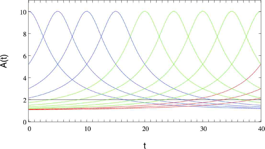
Figure 19.— Examples for the distributions of events within the time interval of the survey, for the standard definition and the maximum light curve definition. The magnification threshold is chosen as ${A_{\mathrm{T}}}=2$. The green light curves are events for both definitions, the blue ones only for the maximum light curve definition, and the red ones only for the standard definition. Of course, in both cases the times, when the events occur are homogeneously distributed within the survey time. The event time, however, is not equal to the time of light curve maximum in the standard definition case. It may happen, the light curve maxima is attained only after the survey has ended (red curves).

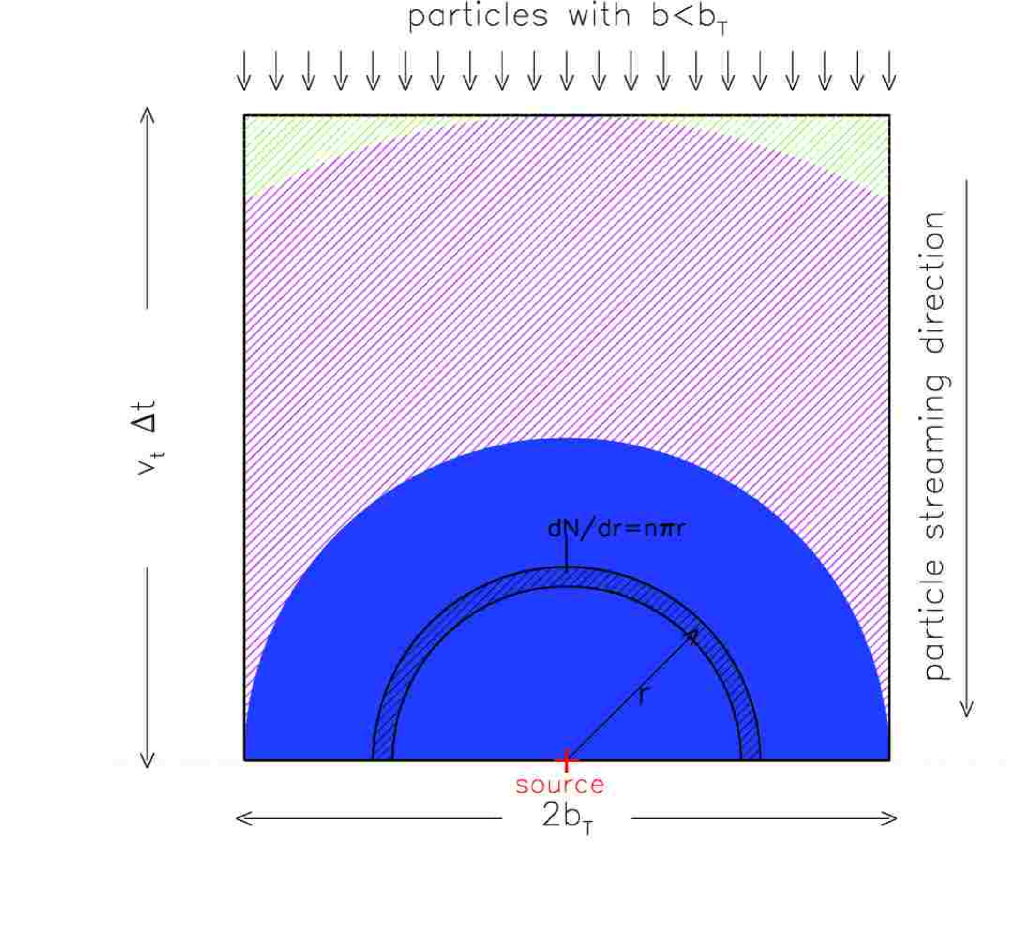
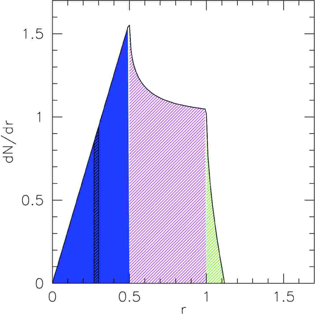
Figure 20.— These two figures illustrate how the impact parameter distribution and the radial distribution of lenses that become events in the maximum light curve definition are related. In the left panel we choose as an example a coherent particle flow with velocities ${v_{\mathrm{t}}}$ in one direction. Those particles that have an impact parameter $b\leq{b_{\mathrm{T}}}$ and will attain their minimum distance to the source within the survey time interval $\Delta t$ are contained in the black box. Three areas have been shaded with blue, magenta, and green. The same colors have been used in the right panel to show in which part of the radial distribution function the events enter.

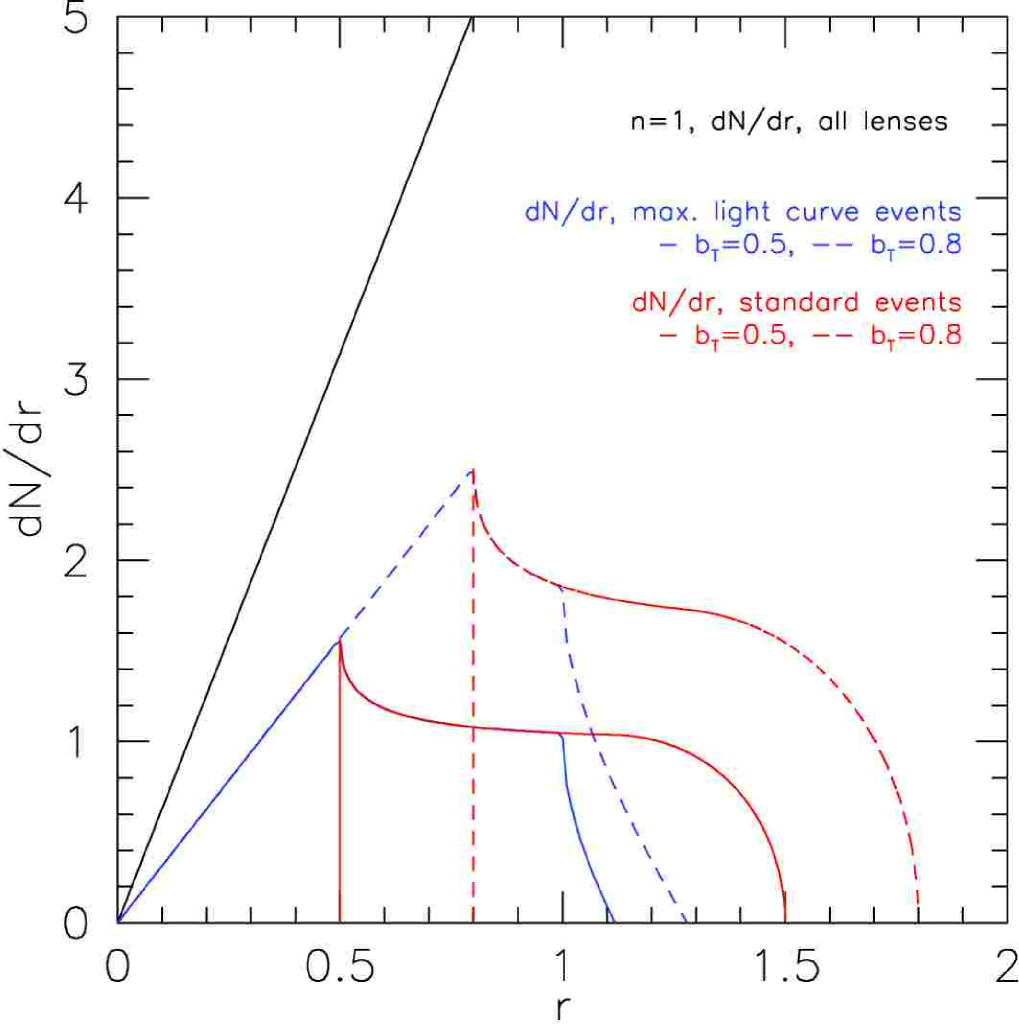
Figure 21.— Number of lenses per radius interval (black) and number of lenses causing events per radius interval. Curves for the standard definition are in red, and for the maximum light curve definition are in blue. Length scales are in arbitrary units, the density is chosen such that it equals $n=1$ in these units, and the velocities are chosen such that ${{v_{\mathrm{t}}}{\Delta t}}=1$ holds. The thresholds for the microlensing tube radius and the maximum impact parameter have been chosen as ${b_{\mathrm{T}}}=0.5$ (solid lines) and ${b_{\mathrm{T}}}=0.8$ (dashed lines). The integral of the corresponding red and blue curves coincide and give the number of lenses that cause events within $\Delta t$. For the standard definition (the locations of) the lenses that cause events with a higher magnification threshold are not all a subset of those with a lower magnification threshold. In addition, lenses that are already within the microlensing tube never will cause any event for the standard definition (implying the lower cutoff). The red and blue curves shown here are straightforwardly obtained analytically (derivation not shown in this paper).

We now consider events with a threshold ${b_{\mathrm{T}}}$ for both event definitions. We calculate the location of those lenses at survey begin that become events within the survey time interval. We assume the lenses to be distributed in a plane and to have velocities ${{v_{\mathrm{t}}}{\Delta t}}=1$. Length scales are given in arbitrary units and the density of lenses is assumed to equal $n=1$ in these units. The number of lenses per radius interval is $\frac{dN}{dr}=2\pi r$. This curve is shown in black in Figure 21.

The blue and red curves show the number of those lenses per radius interval that become events within ${\Delta t}$ in the new and the standard definition, respectively. For the standard definition, only lenses with ${b_{\mathrm{T}}}\leq r\leq{b_{\mathrm{T}}}+{{v_{\mathrm{t}}}{\Delta t}}$ will become events within ${\Delta t}$, explaining the minimum and maximum radius in Figure 21 (red solid and red dashed curve, for a threshold of ${b_{\mathrm{T}}}=0.5$ and ${b_{\mathrm{T}}}=0.8$, respectively).

In the maximum light curve definition lenses within $0<r<[{b_{\mathrm{T}}}^{2}+({{v_{\mathrm{t}}}{\Delta t}})^{2}]^{1/2}$ can cause events with $b<{b_{\mathrm{T}}}$, explaining the maximal radius in Figure 21 (blue solid and blue dashed curves, for the threshold of ${b_{\mathrm{T}}}=0.5$ and ${b_{\mathrm{T}}}=0.8$, respectively). The relation between the features in the radial distribution of lenses becoming events and the particles motion is shown for the case of a coherent particle stream in Figure 20.

One can also see in Figure 21 that lenses with the higher magnification threshold (corresponding to ${b_{\mathrm{T}}}=0.5$) are a subset of those with the lower magnification threshold (${b_{\mathrm{T}}}=0.8$). In addition, the lenses causing an event within $\Delta t$ are spatially more confined than for the standard definition: the maximum radius from which a lens can cause an event with an impact parameter ${b_{\mathrm{T}}}$ within ${\Delta t}$ is $[{b_{\mathrm{T}}}^{2}+({{v_{\mathrm{t}}}{\Delta t}})^{2}]^{1/2}$ for a relative velocity of ${v_{\mathrm{t}}}$.

Hence, it is obvious that new event definition is more easy to use in simulations, but also more directly linked to observations. On the other hand, one can guess from Figure 21 that the integral of the corresponding blue and red curves in Figure 21 agrees. Therefore, the number of events for both definitions is the same.

This implies that for both event definitions, a magnification threshold ${A_{\mathrm{T}}}$ or impact parameter threshold ${b_{\mathrm{T}}}$ (for a given lens mass) yields the same events (same number of events and same light curve parameters for the events, with exception of the time of maximum); only the lenses that cause the events are different in both definitions. Since it is not relevant where the lenses that cause events have come from, one can conveniently switch definitions.

Appendix B Modeling of M31

B.1. Density Distribution

This section contains our models for the bulge, disk and halo density of M31 and comparison with observations. We show that taking a bulge with the same total mass as Kent (1989b) and a disk with the same total mass as Kerins et al. (2001) implies mass-to-light ratios for the stellar populations of bulge and disk in good agreement with expectations from population synthesis models. Our bulge model matches the observed surface brightness values of M31 better than previously published analytical models, which is important for the correct self-lensing prediction in the central part of M31. The contributions of the bulge and disk to the rotation curve are almost identical to that shown in Kerins et al. (2001), which allows us to assume the same density distribution for the dark halo as they did.

In this section we use the disk major axis coordinate system $(x_{0},y_{0},z_{0}$; see Fig. 4), which can easily be transformed to the line-of-sight coordinate system using an inclination $i$ of $77^{\circ}$ of M31 (Stanek & Garnavich, 1998).

B.1.1 Bulge of M31

Our M31 bulge model starts from Table I of Kent (1989b), containing the Gunn-r surface brightness and ellipticity values $\rho^{\mathrm{Kent}}_{r}(a)$ and $\epsilon^{\mathrm{Kent}}(a)$ as a function of major-axis distance $a$ to the center of M31. We assumed $50^{\circ}$ for the position angle of the bulge. Figure 22 demonstrates that with

$$\left[\frac{1}{1-\epsilon(a)}\right]^{2}:=0.254\frac{a}{\mathrm{arcmin}}+1.11$$ (B1)

the ellipticity $\epsilon(a)$ (red curve) becomes an excellent approximation of $\epsilon_{r}^{\rm Kent}(a)$ (blue crosses) between $0.5\arcmin$ and $6\arcmin$.

With this relation we convert $(x_{0},y_{0},z_{0})$ to $a$ by solving the quadratic equation $a^{2}=x_{0}^{2}+y_{0}^{2}+\left(0.254a+1.11\right)z_{0}^{2}$,

$$a(x_{0},y_{0},z_{0})=\frac{0.254z_{0}^{2}+\sqrt{0.254^{2}z_{0}^{4}+4\left(x_{0}^{2}+y_{0}^{2}+1.11z_{0}^{2}\right)}}{2}\hskip 28.45274pt[\mathrm{arcmin}],$$ (B2)

with $x_{0}$, $y_{0}$, $z_{0}$ and $a$ in arcminutes.

The three-dimensionally decomposed spatial brightness density profile of the M31 bulge derived by Kent is well approximated by an $a^{1/4}$ law (see Figure 22b). With equation (B2) the bulge mass density becomes

$$\rho_{\mathrm{bulge}}(x_{0},y_{0},z_{0}):=\left\{\begin{array}[]{ll}\rho_{0}\,10^{-0.4(0.97\,a^{1/4})},&\quad a\leq 0.014\arcmin,\\ \rho_{0}\,10^{-0.4(20.4\,a^{1/4}-6.68)},&\quad 0.014\arcmin<a\leq 0.09\arcmin,\\ \rho_{0}\,10^{-0.4(7.1\,a^{1/4}+0.61)},&\quad a>0.09\arcmin,\end{array}\right.$$ (B3)

where

$$\rho_{0}:={\left(\frac{M}{L}\right)}_{{X}}10^{-0.4\left[\rho^{\mathrm{Kent}}_{0,r}-({\mathcal{M}}_{r}-{\mathcal{M}}_{X})-\mathcal{A}_{{X}}-d_{\mathrm{mod}}-{\mathcal{M}}_{\odot,{X}}\right]}\,\frac{{{M}_{\odot}}}{\mathrm{arcsec}^{3}}$$ (B4)

is the central mass density derived from the central brightness density in the $r$ band, $\rho^{\mathrm{Kent}}_{0,r}=15.19\,\mathrm{mag}\,\mathrm{arcsec}^{-3}$ (Kent (1989b), Table I), and $(M/L)_{X}$ is the bulge mass-to-light ratio in a fiducial filter ${X}$, and $({\mathcal{M}}_{r}-{\mathcal{M}}_{X})$ is the color of the bulge population; ${\mathcal{M}}_{\odot,{X}}:=-2.5\log({{{\mathcal{F}}_{\odot}}}_{X}/{F_{\mathrm{Vega}}}_{X})$ is the absolute brightness of the Sun in that filter and $d_{\mathrm{mod}}$ is the distance modulus to M31.

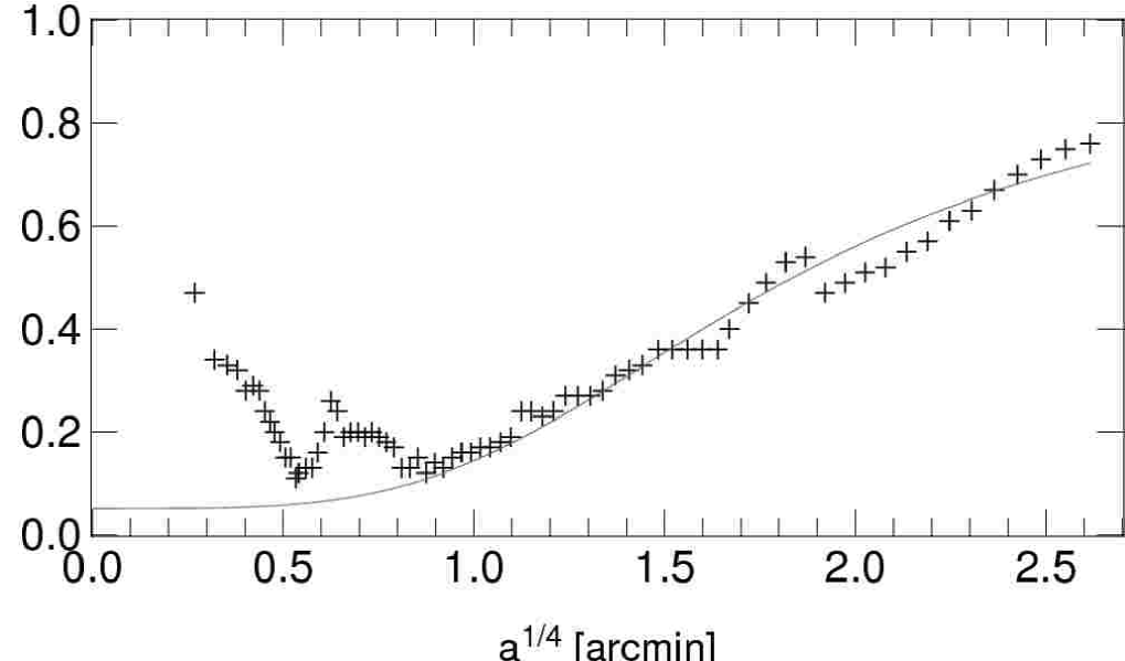
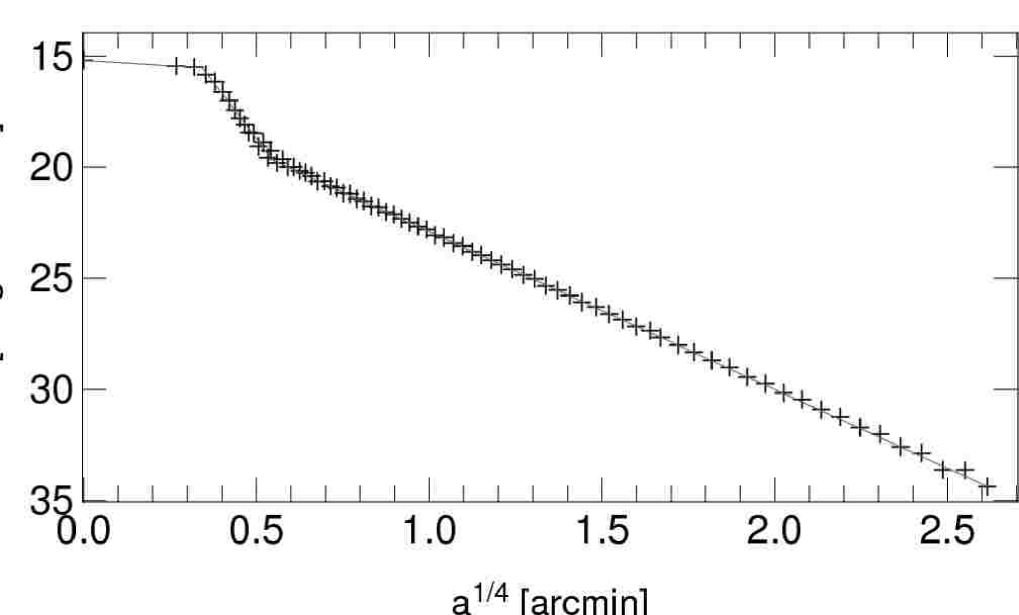
Figure 22.— (a) The gray curve shows our approximation for $\epsilon(a)$ as defined in equation (B1), and the red crosses are the tabulated values of Kent (1989b); within $0.5\arcmin$ and $6\arcmin$ the agreement is excellent. (b) Bulge surface brightness as tabulated by Kent (1989b) is shown with crosses, and our approximation from equation (B3) as a gray curve.

Table 4Mass-to-Light Conversion Ratio for the M31 Bulge Model

	Distance
${M}_{\mathrm{tot}}/{{M}_{\odot}}$	(kpc)	Band ${X}$	$({\mathcal{M}}_{r}-{\mathcal{M}}_{X})$	$\mathcal{A}_{{X}}$	$L_{\mathrm{tot},{X}}/L_{\odot,{X}}$	$(M/L)_{{X}}$	Comment
$4\times 10^{10}$	690	$r$	0	0	$6.61\times 10^{9}$	6.05	Kent’s model using eq. (B4)
$4\times 10^{10}$	770	$R$	0.59	0.36	$13.5\times 10^{9}$	2.96

Kent (1989b) fixes the bulge mass to $4\times 10^{10}\,{{M}_{\odot}}$, which for $d_{\mathrm{mod}}=24.19\,\mathrm{mag}$ ($690\,\mathrm{kpc}$) and without correcting for dust extinction implies a $(M/L)_{r}$-ratio of $6.05$ (using our analytic approximation for $\rho_{\mathrm{bulge}}$) and $5.5-6.6$ (integrating the tabulated values of Kent and estimating the maximal uncertainties due to the coarseness of the table). Using the favored distance to M31 ($d_{\mathrm{mod}}=770\,\mathrm{kpc}$) and applying reasonable extinction values, the dust corrected mass-to-light ratios reduce to lower values (for a constant bulge mass of $4\times 10^{10}\,{{M}_{\odot}}$, see Table 4).

The $R$ band values were obtained with $R_{\odot}=4.42\,\mathrm{mag}$, $({\mathcal{M}}_{r}-{\mathcal{M}}_{R})=0.43+0.15(B-V)=0.59$ (Moro & Munari, 2000), and a bulge color of $(B-V)\approx 1.05$ (Walterbos & Kennicutt, 1987).

According to Han (1996) the effect of an asymmetric bulge light extinction caused by the highly inclined M31 disk is negligible. We therefore adopt his values for the mean internal extinctions toward the bulge in the $V$ and $I$ bands of $\mathcal{A}_{V}=0.24\,\mathrm{mag}$ and $\mathcal{A}_{I}=0.14\,\mathrm{mag}$ and interpolate to the $R$ band which yields $\mathcal{A}_{R}=0.19$. With the foreground extinction of $\mathcal{A}_{R}=0.17$ (Schlegel et al., 1998) the total extinction becomes $\mathcal{A}_{R}=0.36$. In this case, the mass-to-light ratio corresponding to Kent’s bulge mass becomes $(M/L)_{R}=2.96$ (line 2 in Table 4). This value is close to that [$(M/L)_{R,\mathrm{stellar}}=2.67$] one would obtain for a $12\,\mathrm{Gyr}$ old, $Z=2Z_{\odot}$ metallicity single stellar population (SSP; see Girardi et al. (2002)) for a Zoccali et al. (2000) mass function (MF) (see §§ B.2.1 and B.3).

We conclude that a normalization (equation (B4)) of

$$\rho_{0}=2.07\times 10^{6}\,{{M}_{\odot}}\,\mathrm{arcsec}^{-3}=3.97\times 10^{4}\,{{M}_{\odot}}\,\mathrm{pc}^{-3},$$ (B5)

which reproduces Kent’s bulge mass of $M=4\times 10^{10}\,{{M}_{\odot}}$, is a reasonable assumption and represents an upper limit for the luminous matter in the bulge.

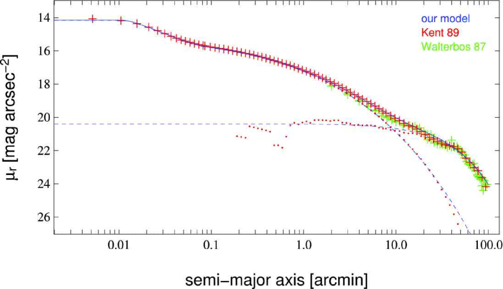
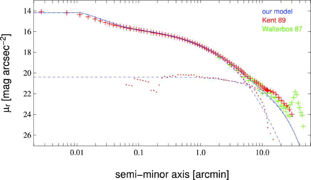
Figure 23.— Surface-brightness profile of M31 in the $r$ band: red crosses are Kent’s $r$ band data for the central region of M31; green crosses are the Walterbos & Kennicutt (1987) data (their Table V) transformed to the $r$ band. The left and right panels show the profiles along semi-major and semi-minor axis, respectively. Kent has decomposed the surface brightness profile into the bulge and disk component (red dots). For comparison we have superposed our bulge and disk surface brightness models from Eqs. B3 and B6. With the exception of spiral arm imprints, they match the observations extremely well.

B.1.2 Disk of M31

Like Kerins et al. (2001), we model the disk by a $\mathrm{sech}^{2}$ law,

$$\rho_{\mathrm{disk}}(x_{0},y_{0},z_{0})=\rho_{0}\exp{\left(-\frac{\sigma(x_{0},y_{0})}{h_{\sigma}}\right)}\,\mathrm{sech}^{2}{\left(\frac{z_{0}}{h_{z}}\right)},$$ (B6)

with $\sigma(x_{0},y_{0})={\left(x_{0}^{2}+y_{0}^{2}\right)}^{1/2}$ being the radial distance in the disk plane inclined by $77^{\circ}$; the radial scale length $h_{\sigma}=28.57\arcmin$ and the vertical scale lengths $h_{z}=1.34\arcmin$ are equivalent to Kerins et al. (2001) values $h_{\sigma}=6.4\,\mathrm{kpc}$ and $h_{z}=0.3\,\mathrm{kpc}$ for a M31 distance of 770 kpc. Adopting a central brightness density of the disk in the $r$ band $\rho^{\mathrm{Kent}}_{0,r}=27.39\,\mathrm{mag}\,\mathrm{arcsec}^{-3}$ yields a surface brightness profile that matches the data of Kent (1989b) on the major axis and that agrees well with his central surface brightness of $\mu_{0}=20.4\,\mathrm{mag}$ in the $r$ band. Spiral arms and dust explain the discrepancies at the minor axis (see Figure 23). We assumed $38^{\circ}$ for the position angle of the disk.

As for the bulge, we transform the luminosity density to matter density, using the disk color $({\mathcal{M}}_{r}-{\mathcal{M}}_{X})$, disk extinction $\mathcal{A}_{X}$, and disk mass-to-light ratio $(M/L)_{X}$

$$\rho_{0}={\left(\frac{M}{L}\right)}_{X}10^{-0.4(\rho^{\mathrm{Kent}}_{0,r}-({\mathcal{M}}_{r}-{\mathcal{M}}_{X})-\mathcal{A}_{X}-d_{\mathrm{mod}}-{\mathcal{M}}_{\odot,{X}})}\frac{{{M}_{\odot}}}{\mathrm{arcsec}^{3}},$$ (B7)

with the absolute brightness of the Sun ${\mathcal{M}}_{\odot,{X}}$, and the distance modulus $d_{\mathrm{mod}}$ to M31.

Table 5Mass-to-Light Conversion Ratio for the M31 Disk Model

	Distance
${M}_{\mathrm{tot}}/{{M}_{\odot}}$	(kpc)	Band ${X}$	$({\mathcal{M}}_{r}-{\mathcal{M}}_{X})$	$\mathcal{A}_{{X}}$	$L_{\mathrm{tot},{X}}/L_{\odot,{X}}$	$(M/L)_{{X}}$	Comment
$16\times 10^{10}$	690	gunn $r$	0	0	$1.4\dots 1.7\times 10^{10}$	$11.3\dots 9.6$	for Kent’s max. disk mass
$3.09\times 10^{10}$	690	gunn $r$	0	0	$1.34\times 10^{10}$	2.31	for Kerins’s disk mass
$3.09\times 10^{10}$	770	$R$	0.54	0.68	$3.5\times 10^{10}$	0.88

We normalize equation (B7) with

$$\rho_{0}=10.4\,{{M}_{\odot}}\,\mathrm{arcsec}^{-3}=0.2\,{{M}_{\odot}}\,\mathrm{pc}^{-3}$$ (B8)

to obtain the same disk mass as Kerins et al. (2001) $M_{\mathrm{disk}}=\int\int\rho\,dz\,d\sigma=4\pi\rho_{0}h_{z}h_{\sigma}^{2}=3.09\times 10^{10}\,{{M}_{\odot}}$. Table 5 demonstrates that this normalization results in a mass-to-light ratio that is expected for the disk population.

With $E(B-V)=0.22$ (Stephens et al., 2003) we obtain $\mathcal{A}_{V}=3.1E(B-V)=0.682$ for the extinction in the M31 disk. This translates to $\mathcal{A}_{R}=0.748\,\mathcal{A}_{V}=0.51$ (Binney & Merrifield, 1998). Adding the foreground extinction, $\mathcal{A}_{R}=0.17$ (Schlegel et al., 1998), we obtain $\mathcal{A}_{R}=0.68$ for the total extinction for sources residing in the disk of M31. Using that extinction, the M31 distance of 770 kpc and the central luminosity density of $\rho^{\mathrm{Kent}}_{0,R}=26.86\,\mathrm{mag}\,\mathrm{arcsec}^{-3}$ [obtained from $\rho^{\mathrm{Kent}}_{0,r}$ and $({\mathcal{M}}_{r}-{\mathcal{M}}_{R})=0.53$ for a disk color $(B-V)\approx 0.7$; Walterbos & Kennicutt (1987)], we get a disk luminosity of $L_{\mathrm{tot},R}/L_{\odot,R}=3.5\times 10^{10}$. For the disk mass of Kerins et al. (2001), our $(M/L)_{R}$ ratio becomes 0.88. This mass-to-light ratio is well consistent with a theoretical $(M/L)_{R,\mathrm{stellar}}=0.61$ for a $2\,\mathrm{Gyr}$ old, solar metalicity SSP disk population (based on Gould et al. (1997) and Girardi et al. (2002)).

We also summarize the maximum disk model of Kent (1989b) in Table 5 (first row). This model implies a 4 times higher $(M/L)_{r}$-ratio, which is hard to reconcile with population synthesis models.

Note that the results from Han & Gould (1996a) are not easy to compare with ours: they used a double exponential disk with $\rho_{0}=0.35\,{{M}_{\odot}}\,\mathrm{pc}^{-3}$, $h_{z}=0.4$ kpc, and $h_{\sigma}=6.4$ kpc corresponding to a disk mass of $7.2\times 10^{10}\,{{M}_{\odot}}$. At the same time their bulge is also more massive than ours ($4.9\times 10^{10}\,{{M}_{\odot}}$).

B.1.3 Halo of M31

Our density models for the bulge and disk differ only slightly (e.g., in the central region) from that of Kerins et al. (2001). The contributions to the rotation velocity resulting from the different populations are therefore very much the same as in the Kerins et al. (2001) model. This implies that we can use the halo density distribution from Kerins et al. (2001) to obtain a halo model consistent with the observed M31 rotation curve. This halo density distribution is that of an isothermal sphere with a core radius of $r_{\mathrm{c}}=2\,\mathrm{kpc}$:

$$\rho_{\mathrm{halo}}(x_{0},y_{0},z_{0})=\frac{\rho_{0}}{1+\left(r/r_{\mathrm{c}}\right)^{2}},\quad r\leq 200\,\mathrm{kpc},$$ (B9)

with $r=(x_{0}^{2}+y_{0}^{2}+z_{0}^{2})^{1/2}$, $r_{\mathrm{c}}=2\,\mathrm{kpc}$, and $\rho_{0}=0.23\,{{M}_{\odot}}\,\mathrm{pc}^{-3}$. Figure 24 shows the overall rotation curve of our model.

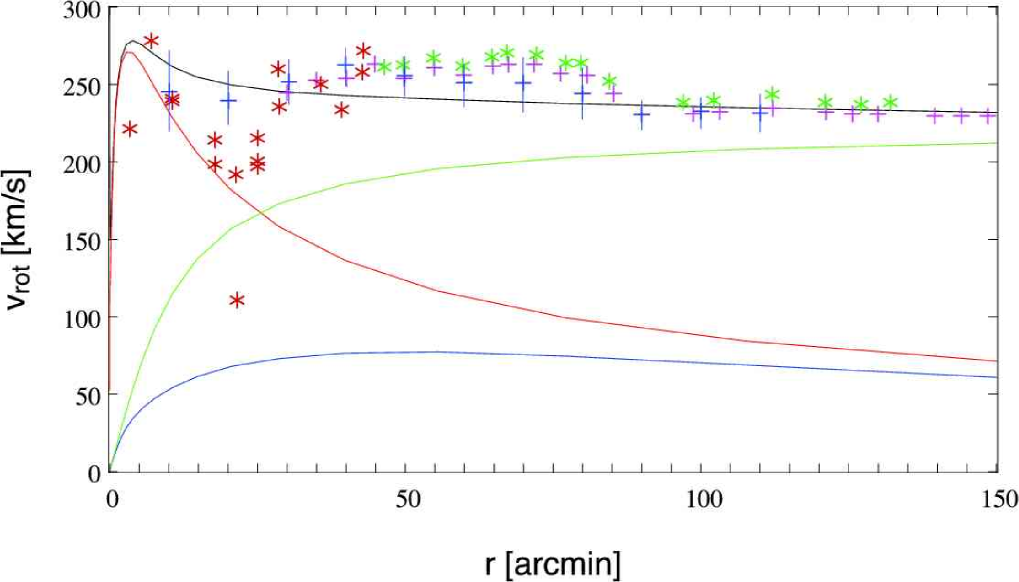
Figure 24.— Overall rotation curve of our model (black curve) and its contributions of the bulge (red), disk (blue), and halo (green). These rotation curves match with Fig. 3b in Kerins et al. (2001). In red crosses we show the data points derived from CO measurements of Loinard et al. (1995); in green, HI measurements from Brinks & Burton (1984); in blue, averaged data points from Widrow et al. (2003) (based on Kent (1989a), and Braun (1991)); in magenta, the data points of Kerins et al. (2001) (based on Kent (1989b)).

In the model of Han & Gould (1996a) the core radius of the halo is much larger ($r_{\mathrm{c}}=6.5\,\mathrm{kpc}$) to compensate for their higher disk and bulge mass in order to match the rotation curve of M31.

B.1.4 Halo of the Milky Way

The halo of the Milky Way (MW) is also modeled as a cored isothermal sphere,

$$\rho_{\mathrm{MW}}({D_{\mathrm{ol}}})=\frac{\rho_{0}}{1+\left(r/r_{\mathrm{c}}\right)^{2}},\quad r<200\,\mathrm{kpc},$$ (B10)

where we choose a core radius of $r_{\mathrm{c}}=2\,\mathrm{kpc}$ as used in Han & Gould (1996a) and Gyuk & Crotts (2000).

The central density is taken from (Han & Gould, 1996a):

$$\rho_{0}=0.0079\,{{M}_{\odot}}\,\mathrm{pc}^{-3}\,\left[1+\left(\frac{r_{\odot}}{r_{\mathrm{c}}}\right)^{2}\right]=0.1343\,{{M}_{\odot}}\,\mathrm{pc}^{-3}.$$ (B11)

We convert the Galactocentric distance $r$ to our line-of-sight coordinate system according to

$$r({D_{\mathrm{ol}}})=\sqrt{r_{\odot}^{2}-2r_{\odot}{D_{\mathrm{ol}}}\cos(l)\cos(b)+{D_{\mathrm{ol}}}^{2}},$$ (B12)

using the M31 Galactic coordinates $l=121.14988^{\circ}$, $b=-21.61707^{\circ}$ and the solar Galactocentric distance $r_{\odot}=8\,\mathrm{kpc}$ (Bahcall et al., 1983).

B.2. The Mass Function

B.2.1 The Mass Function for the bulge and disk sources

For the M31 bulge we take the mass function (MF) $\xi\sim M^{-1.33}$ of Zoccali et al. (2000), which was derived for the Galactic bulge. The MF is cut off at $0.01\,{{M}_{\odot}}$ at the lower end and at the MS turnoff $1.01\,{{M}_{\odot}}$ at the upper end for a 12 Gyr old SSP with $Z=2Z_{\odot}$.

We describe the disk with a Gould MF, $\xi\sim M^{-2.21}$, which has a flattening $\xi\sim M^{-0.56}$ below $0.59\,{{M}_{\odot}}$ (Gould et al., 1997). We cut the disk MF at $0.01$ and $1.71\,{{M}_{\odot}}$ (2 Gyr old SSP with $Z=Z_{\odot}$), respectively. Of course, the number of stars with a given mass changes for different cut off values or for alternative mass functions (e.g., Chabrier (2003)). The investigation of halo-lensing and self-lensing rates for different MFs is not a subject of that paper.

B.2.2 The Mass Function for the Halo

The mass function $\xi({M})$ for the potential MACHO population residing in the halo of M31 is of course unknown. In this paper we simply assume that the halo consists of one mass objects ${{M}_{0}}$ only,

$$\xi({M})=\frac{\delta({M}-{{M}_{0}})}{{{M}_{0}}},$$ (B13)

satisfying the normalization constraint

$$\int{M}\,\xi({M})\,d{M}=1.$$ (B14)

B.3. The Luminosity Function and CM Diagram

We use a stellar LF obtained from isochrones of the Padova database of stellar evolutionary tracks and isochrones given by Girardi et al. (2002) (based on Marigo & Girardi (2001)).

The luminosity function can be extracted from the mass function $\xi({M})$ discussed in § B.2.1. Using the mass-magnitude relation provided by theoretical stellar isochrones each mass bin $[{M}_{i},{M}_{i+1}]$ of stars is connected to a absolute brightness bin $[{\mathcal{M}}_{i},{\mathcal{M}}_{i+1}]$:

$$\begin{array}[]{l}\int\limits_{{\mathcal{M}}_{i}}^{{\mathcal{M}}_{i+1}}\Phi({\mathcal{M}})\,d{\mathcal{M}}\stackrel{{\scriptstyle!}}{{=}}\int\limits_{{M}_{i}}^{{M}_{i+1}}\xi({M})\,d{M}\end{array}$$ (B15)

and therefore,

$$\Phi({\mathcal{M}})\approx\frac{\int\limits_{{M}_{i}({\mathcal{M}}_{i})}^{{M}_{i+1}({\mathcal{M}}_{i+1})}\xi({M})\,d{M}}{{\mathcal{M}}_{i+1}-{\mathcal{M}}_{i}}\hskip 28.45274pt{\mathcal{M}}_{i}\leq{\mathcal{M}}\leq{\mathcal{M}}_{i+1}.$$ (B16)

For the bulge we assumed a 12 Gyr old SSP with $Z=2Z_{\odot}$ (isoc_z040s.dat), which leads to good results for the stellar content of the bulge (C. Maraston 2004, private communication).

For the disk we used for simplicity a 2 Gyr old SSP with $Z=Z_{\odot}$ (isoc_z019m.dat; see footnote 31) leading to acceptable results for the disk data shown in (Williams (2002); fields INNER, NGC224-DISK, NGC224-POS2, G287, G11, G272, G87, K108, and G33).

With the mass function $\xi({M})$ and the luminosity function $\Phi({\mathcal{M}})$ we obtain the mass-to-light ratio

$${\left(\frac{M}{L}\right)}=\frac{\int\limits_{{M}_{\mathrm{min}}}^{{M}_{\mathrm{max}}}{M}\,\xi({M})\,d{M}\,/{M}_{\odot}}{\int\limits_{-\infty}^{+\infty}{F_{\mathrm{Vega}}}10^{-0.4{\mathcal{M}}}\Phi({\mathcal{M}})\,d{\mathcal{M}}\,/{{\mathcal{F}}_{\odot}}}=\frac{\int\limits_{{M}_{\mathrm{min}}}^{{M}_{\mathrm{max}}}{M}\,\xi({M})\,d{M}\,/{M}_{\odot}}{<{\mathcal{F}}>\,\int\limits_{-\infty}^{+\infty}\Phi({\mathcal{M}})\,d{\mathcal{M}}\,/{{\mathcal{F}}_{\odot}}}.$$ (B17)

For a bulge MF as in § B.2.1 we get a characteristic flux $<{\mathcal{F}}_{R}>=0.20{{\mathcal{F}}_{\odot,R}}$, yielding a $(M/L)$ in the $R$ band of $(M/L)_{R}=2.67$ and a $(B-V)=1.14\,\mathrm{mag}$. For a disk MF as in § B.2.1 we get a characteristic flux $<{\mathcal{F}}_{R}>=0.67{{\mathcal{F}}_{\odot,R}}$, yielding a $(M/L)$ in the $R$ band of $(M/L)_{R}=0.61$ and a $(B-V)=0.88\,\mathrm{mag}$.

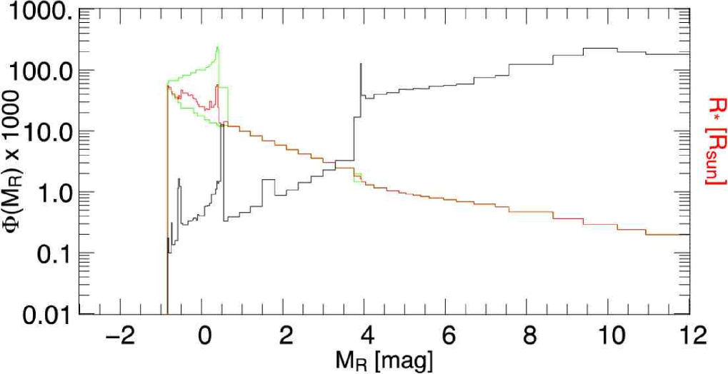
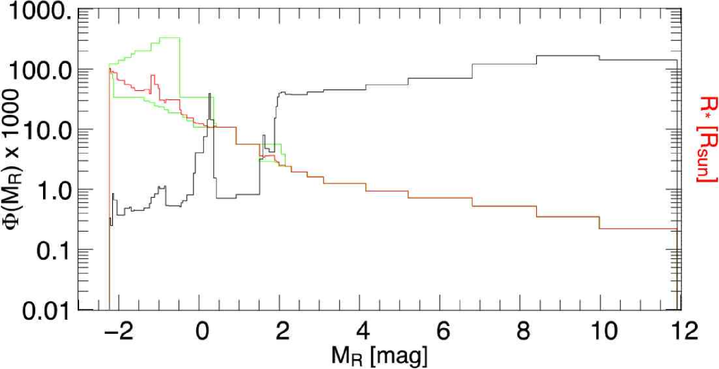
Figure 25.— Theoretical LF in the $R$ band $\tilde{\Phi}_{R}({\mathcal{M}})$. Left: bulge for a 12 Gyr old SSP of 2 $Z_{\odot}$ metalicity. Right: disk for a 2 Gyr old SSP of 1 $Z_{\odot}$ metalicity. In red and green we show the values of the stellar radii obtained with § B.4 and the theoretical luminosities for the stars of the model SSP. The red line shows the average radius $\overline{R}_{\ast}$ according to equation (B19). In green we give the minimal and maximal radii of stars (reflecting the different values in color space) in the particular magnitude range. The LF was scaled by a factor of 1000 to show the two different histograms with the same scaling. The unit of the LF is number of stars per magnitude, the radii distribution is given in solar radii.

Note that other values of ${M}_{\mathrm{min}}$ and ${M}_{\mathrm{max}}$ give different mass-to-light ratios, as the decrease of ${M}_{\mathrm{min}}$ increases only the mass of the population, but not its luminosity. We show the LF for the bulge population in Figure 25, along with the stellar radii data (see § B.4). Note that the faint cutoff of $\Phi({\mathcal{M}})$ affects the characteristic luminosity $<{\mathcal{F}}>$ but at the same time the normalization of $\tilde{\Phi}({\mathcal{M}})=\Phi({\mathcal{M}})/\int\Phi({\mathcal{M}})d{\mathcal{M}}$. Therefore, the number of bright stars, ${\mathcal{F}}_{\mathrm{tot}}<{\mathcal{F}}>^{-1}\int_{\mathrm{bright}}\tilde{\Phi}({\mathcal{M}})\,d{\mathcal{M}}$, is nearly not affected by changing the faint cutoff.

Using equation (43) we calculate the projected densities of bulge and disk stars brighter than ${\mathcal{M}}_{R}\leq 0\,\mathrm{mag}$ and show the results in Figure 26; basically at any position monitored by WeCAPP there is more than one bright star per square arcsec each from bulge and disk. This demonstrates that crowding in the central bulge is very severe even for the brightest stars with ${\mathcal{M}}_{R}\leq 0\,\mathrm{mag}$ and even if image PSFs are small.

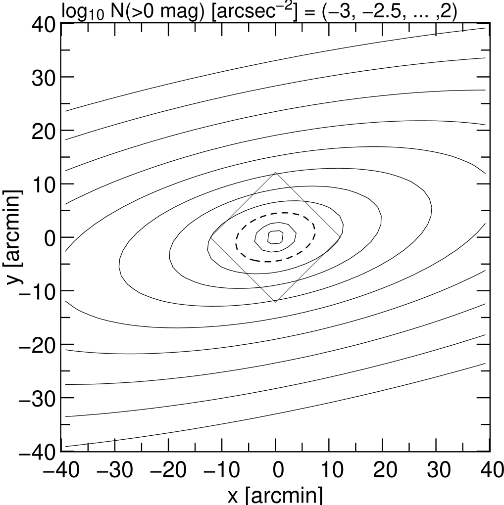
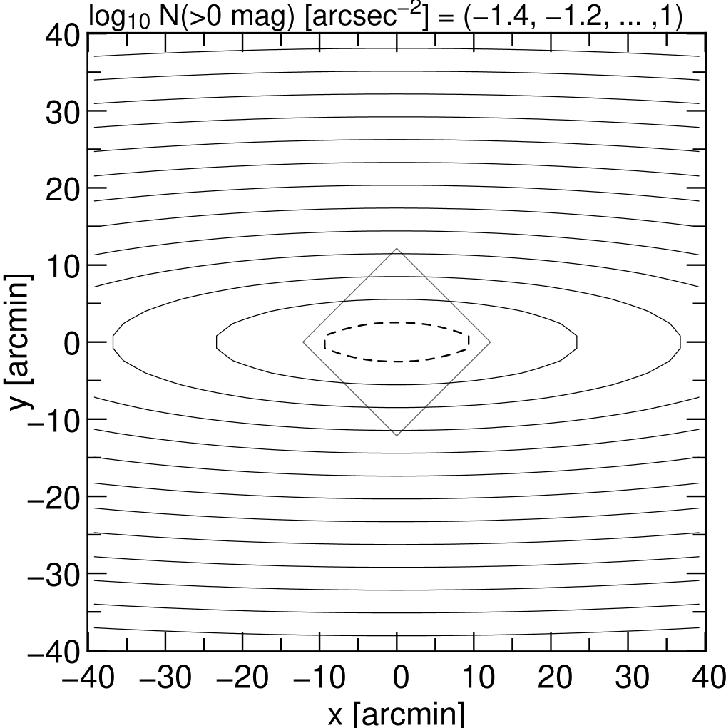
Figure 26.— Number density of bulge stars (left) and disk stars (right) brighter than ${\mathcal{M}}_{R}\leq 0\,\mathrm{mag}$ in units of stars arcsec^-2. The contours show the values of $\left.d^{2}N/(dx\,dy)\right|_{{\mathcal{M}}_{R}\leq 0}=\int_{-\infty}^{0}\int_{0}^{\infty}\tilde{\Phi}({\mathcal{M}}_{R})\,n_{s}(x,y,{D_{\mathrm{os}}})\,d{D_{\mathrm{os}}}\,d{\mathcal{M}}_{R}$ and were obtained from the number density and luminosity functions of the bulge and disk component of M31. The WeCAPP field, a square of $17.2\arcmin$, is shown as a box. The dashed contour outline a density of the ${\mathcal{M}}_{R}\leq 0$ stars of 10 stars/arcsec² and demonstrate that one cannot resolve even giants in the central M31 field for the majority of ground-based data. The coordinates are that of the intrinsic M31 system (see Figure 4).

B.4. Radius-Brightness Relations for Stars

For the inclusion of finite source effects one needs the radius-brightness relation of stars. The radius can easily be correlated to the brightness (and to the luminosity function) using $\log(L_{i})$ and $\log(T_{\mathrm{eff},i})$ given in the theoretical stellar isochrones (see § B.3)

$$R_{\ast}({\mathcal{M}}_{i},{\mathcal{C}}_{i})=\frac{10^{\left[\log L_{i}+\log L_{i+1}\right]/4}}{\sqrt{4\pi\sigma_{\mathrm{B}}}\,10^{\log T_{\mathrm{eff},i}+\log T_{\mathrm{eff},i+1}}}\hskip 28.45274pt{\mathcal{M}}_{i}\leq{\mathcal{M}}\leq{\mathcal{M}}_{i+1}\,,{\mathcal{C}}_{i}\leq{\mathcal{C}}\leq{\mathcal{C}}_{i+1}.$$ (B18)

If we want to account for finite source effects without having any color information, e.g., equation (63), we use a color-averaged source radius $\overline{R}_{\ast}$,

$$\overline{R}_{\ast}({\mathcal{M}})=\int{p_{\mathrm{cmd}}}({\mathcal{M}},{\mathcal{C}})\,R_{\ast}({\mathcal{M}},{\mathcal{C}})\,d{\mathcal{C}},$$ (B19)

and replace $R_{\ast}({\mathcal{M}},{\mathcal{C}})$ with $\overline{R}_{\ast}({\mathcal{M}})$ in Eqs. 66 and 67 (see Figure 25).

B.5. The Velocity Distributions for the M31 Components

The random velocity components of bulge, disk, and halo are assumed to be of Gaussian shape with dispersions taken from Kerins et al. (2001):

$$\begin{array}[]{ll}\sigma_{\mathrm{bulge}}=100\,\mathrm{km\ s}^{-1},&\sigma_{\mathrm{disk}}=30\,\mathrm{km\ s}^{-1},\\ \sigma_{\mathrm{halo}}=166\,\mathrm{km\ s}^{-1},&\sigma_{\mathrm{MW-halo}}=156\,\mathrm{km\ s}^{-1}.\end{array}$$ (B20)

In addition, we account for rotation in bulge and disk of $v_{\mathrm{rot,bulge}}=30\,\mathrm{km\ s}^{-1}$ and $v_{\mathrm{rot,disk}}=235\,\mathrm{km\ s}^{-1}$ (Kerins et al., 2001). In a previous work Han & Gould (1996a) used $\sigma_{\mathrm{halo}}=170\,\mathrm{km\ s}^{-1}$ for the halo, but a value of $\sigma_{\mathrm{bulge}}=156\,\mathrm{km\ s}^{-1}$ for the bulge and disk (based on Lawrie (1983)).

In the following two sections we derive the relative source-lens velocity $v_{0}$ taking into account rotation of the source and lens objects and the observers motion. The combination of all contributions results in one movement depending on

$$v_{0}({D_{\mathrm{os}}},{D_{\mathrm{ol}}},v_{\mathrm{rot,l}},v_{\mathrm{rot,s}},v_{\odot-\mathrm{M31}}).$$ (B21)

B.5.1 Additional Rotation for Lenses and Sources

The additional rotation of the lens system $v_{\mathrm{rot,l}}$ (for bulge and disk lenses) and/or of the source system $v_{\mathrm{rot,s}}$ changes the relative velocity $v_{0}$. For the calculation of the effect we first have to transform the positional components of a lens located at ($x,y,z:={D_{\mathrm{ol}}}-d_{\mathrm{m31}}$) along the line-of-sight to the components ($x_{0},y_{0},z_{0}$) in the M31 system. In the internal system the position is given by

$$x_{0}=x,\quad y_{0}=y\cos{i}-z\sin{i},\quad z_{0}=y\sin{i}+z\cos{i},$$ (B22)

with inclination angle $i=77^{\circ}$ and the distance to M31 $d_{\mathrm{m31}}=770$ kpc. Projecting on the base $\rho=(x_{0}^{2}+y_{0}^{2})^{1/2}$, the rotation angle can be expressed as $\omega=\arccos(x_{0}/\rho)=\arcsin(y_{0}/\rho)$.

Reprojecting the components of the rotation velocity $v_{x}$ and $v_{yz}$ (calculated for a clockwise rotation)

$$v_{x}=v_{\mathrm{rot}}\sin{\omega}=-\frac{y_{0}}{\sqrt{x_{0}^{2}+y_{0}^{2}}}\,v_{\mathrm{rot}},\quad v_{yz}=\sqrt{v_{\mathrm{rot}}^{2}-v_{x}^{2}}=\frac{x_{0}}{\sqrt{x_{0}^{2}+y_{0}^{2}}}\,v_{\mathrm{rot}},$$ (B23)

to the $y$- and $z$- plane yields

$$\begin{array}[]{l}v_{y}=v_{yz}\cos{i},\quad v_{z}=v_{yz}\sin{i},\end{array}$$ (B24)

which depends on the position along the line-of-sight ($x,y,z$). To combine this velocity vector $(v_{x},v_{y},v_{z})$ with all other velocities (see § B.5.2) it has to be projected to the lens plane.

B.5.2 Observer’s Motion

Finally, we have to account for the transversal velocity of M31 $v_{\mathrm{M31}}$ arising from the observers motion against M31. A hypothetical star on a circular orbit at solar distance (local standard of rest, LSR) has velocity $v_{l}(R_{\odot})=220\pm 15\,\mathrm{km\ s}^{-1}$. The Sun is moving with $v_{\odot}=16.5\,\mathrm{km\ s}^{-1}$ relative to the LSR toward the directions $l=53^{\circ}$, $b=25^{\circ}$ (Binney & Tremaine, 1987). For simplicity we neglect the contributions to the Galactic height (see Figure 27) and calculate the transversal velocity of M31 as

$$\begin{array}[]{ll}v_{\odot-\mathrm{M31}}\approx&(220\,\mathrm{km\ s}^{-1})\,\sin(l_{\mathrm{M31}}-90^{\circ})+16.5\,\mathrm{km\ s}^{-1}\,\sin(121^{\circ}-l_{\mathrm{LSR}})=129\,\mathrm{km\ s}^{-1},\end{array}$$ (B25)

with the Galactic coordinates of M31 $l_{\mathrm{M31}}=121.2^{\circ}$ and $b_{\mathrm{M31}}=-21.6^{\circ}$. The relative velocity between the velocity distribution of the lenses and the sources is calculated by projecting $v^{p}_{\odot-\mathrm{M31}}$ to the lens plane

$$v^{p}_{\odot-\mathrm{M31}}\approx\frac{{D_{\mathrm{os}}}-{D_{\mathrm{ol}}}}{{D_{\mathrm{os}}}}129\,\mathrm{km\ s}^{-1}.$$ (B26)

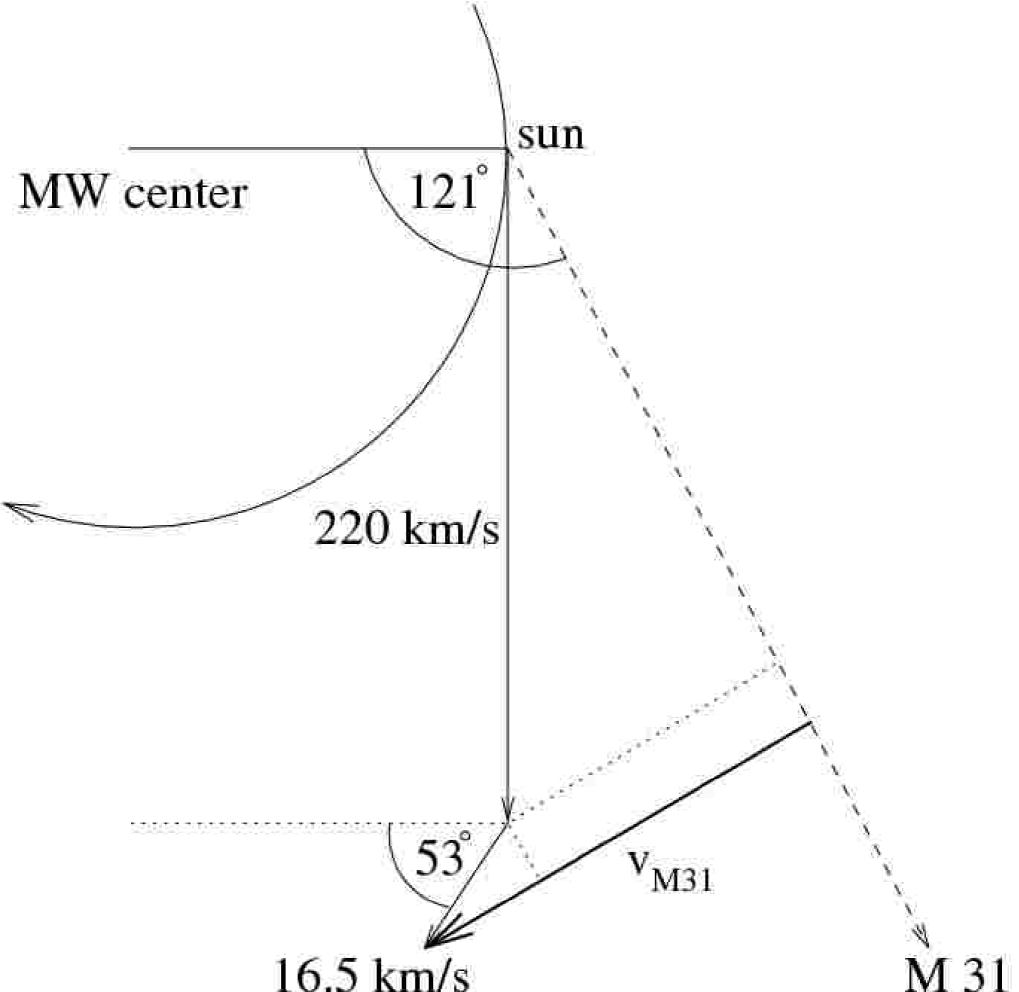
Figure 27.— Geometry of the Galaxy-M31 system. A star at solar distance is assumed to move on a circular orbit with a rotational velocity of $220\,\mathrm{km\ s}^{-1}$ (local standard of rest, LSR). M31 is located at Galactic coordinates $l_{\mathrm{M31}}=121.2^{\circ}$ and $b_{\mathrm{M31}}=-21.6^{\circ}$. The Sun has a velocity of $16.5\,\mathrm{km\ s}^{-1}$ relative to the LSR. The transversal velocity of M31 is shown as $v_{\mathrm{M31}}$.

For lenses residing in M31 this motion is negligible compared to the rotation described in § B.5.1.

References

- Alard (1999) Alard, C. 1999, A&A, 343, 10
- Alard (2001) Alard, C. 2001, MNRAS, 320, 341
- Alard & Guibert (1997) Alard, C. & Guibert, J. 1997, A&A, 326, 1
- Alcock et al. (1997) Alcock, C., Allsman, R. A., Alves, D., et al. 1997, ApJ, 486, 697+
- Alcock et al. (2001a) Alcock, C., Allsman, R. A., Alves, D. R., et al. 2001a, ApJ, 552, 582
- Alcock et al. (2001b) Alcock, C., Allsman, R. A., Alves, D. R., et al. 2001b, ApJS, 136, 439
- Alcock et al. (1995) Alcock, C., Allsman, R. A., Axelrod, T. S., et al. 1995, ApJ, 449, 28
- An et al. (2004) An, J. H., Evans, N. W., Hewett, P., et al. 2004, MNRAS, 351, 1071
- Ansari et al. (2004) Ansari, R., Aurière, M., Baillon, P., et al. 2004, A&A, 421, 509
- Ansari et al. (1999) Ansari, R., Aurière, M., Baillon, P., et al. 1999, A&A, 344, L49
- Ansari et al. (1997) Ansari, R., Auriere, M., Baillon, P., et al. 1997, A&A, 324, 843
- Aubourg et al. (1993) Aubourg, E., Bareyre, P., Brehin, S., et al. 1993, Nat, 365, 623+
- Auriere et al. (2001) Auriere, M., Baillon, P., Bouquet, A., et al. 2001, ApJ, 553, L137
- Bahcall et al. (1983) Bahcall, J. N., Soneira, R. M., & Schmidt, M. 1983, ApJ, 265, 730
- Baltz et al. (2004) Baltz, E. A., Lauer, T. R., Zurek, D. R., et al. 2004, ApJ, 610, 691
- Baltz & Silk (2000) Baltz, E. A. & Silk, J. 2000, ApJ, 530, 578
- Binney & Merrifield (1998) Binney, J. & Merrifield, M. 1998, Galactic Astronomy (Princeton: Princeton Univ. Press)
- Binney & Tremaine (1987) Binney, J. & Tremaine, S. 1987, Galactic Dynamics (Princeton, Princeton Univ. Press)
- Bozza et al. (2000) Bozza, V., Calchi Novati, S., Capaccioli, M., et al. 2000, Mem. Soc. Astron. Italiana, 71, 1113
- Braun (1991) Braun, R. 1991, ApJ, 372, 54
- Brinks & Burton (1984) Brinks, E. & Burton, W. B. 1984, A&A, 141, 195
- Calchi Novati et al. (2003) Calchi Novati, S., Jetzer, P., Scarpetta, G., et al. 2003, A&A, 405, 851
- Calchi Novati et al. (2005) Calchi Novati, S., Paulin-Henriksson, S., An, J., et al. 2005, A&A, 443, 911
- Chabrier (2003) Chabrier, G. 2003, PASP, 115, 763
- Crotts (1992) Crotts, A. P. S. 1992, ApJ, 399, L43
- Crotts & Tomaney (1996) Crotts, A. P. S. & Tomaney, A. B. 1996, ApJ, 473, L87
- de Jong et al. (2004) de Jong, J. T. A., Kuijken, K., Crotts, A. P. S., et al. 2004, A&A, 417, 461
- de Jong et al. (2006) de Jong, J. T. A., Widrow, L. M., Cseresnjes, P., et al. 2006, A&A, 446, 855
- De Marchi et al. (2004) De Marchi, G., Sirianni, R., Gilliland, R., et al. 2004, STScI - Instrument Science Report, ACS 2004-08
- de Rujula et al. (1991) de Rujula, A., Jetzer, P., & Masso, E. 1991, MNRAS, 250, 348
- Dominik (1998) Dominik, M. 1998, A&A, 330, 963
- Dong et al. (2006) Dong, S., DePoy, D. L., Gaudi, B. S., et al. 2006, ApJ, 642, 842
- Fliri et al. (2006) Fliri, J., Riffeser, A., Seitz, S., & Bender, R. 2006, A&A, 445, 423
- Girardi et al. (2002) Girardi, L., Bertelli, G., Bressan, A., et al. 2002, A&A, 391, 195
- Gondolo (1999) Gondolo, P. 1999, ApJ, 510, L29
- Gould (1994a) Gould, A. 1994a, ApJ, 421, L75
- Gould (1994b) Gould, A. 1994b, ApJ, 421, L71
- Gould (1995) Gould, A. 1995, ApJ, 455, 44
- Gould (1996a) Gould, A. 1996a, PASP, 108, 465
- Gould (1996b) Gould, A. 1996b, ApJ, 470, 201+
- Gould et al. (1997) Gould, A., Bahcall, J. N., & Flynn, C. 1997, ApJ, 482, 913
- Gouliermis et al. (2005) Gouliermis, D., Brandner, W., & Henning, T. 2005, ApJ, 623, 846
- Griest (1991) Griest, K. 1991, ApJ, 366, 412
- Gyuk & Crotts (2000) Gyuk, G. & Crotts, A. 2000, ApJ, 535, 621
- Han (1996) Han, C. 1996, ApJ, 472, 108+
- Han & Gould (1996a) Han, C. & Gould, A. 1996a, ApJ, 473, 230+
- Han & Gould (1996b) Han, C. & Gould, A. 1996b, ApJ, 467, 540
- Han et al. (2000) Han, C., Park, S., & Jeong, J. 2000, MNRAS, 316, 97
- Jetzer (1994) Jetzer, P. 1994, ApJ, 432, L43
- Jetzer & Massó (1994) Jetzer, P. & Massó, E. 1994, Physics Letters B, 323, 347
- Joshi et al. (2001) Joshi, Y. C., Pandey, A. K., Narasimha, D., & Sagar, R. 2001, Bull. Astron. Soc. India, 29, 531
- Kent (1989a) Kent, S. M. 1989a, PASP, 101, 489
- Kent (1989b) Kent, S. M. 1989b, AJ, 97, 1614
- Kerins et al. (2001) Kerins, E., Carr, B. J., Evans, N. W., et al. 2001, MNRAS, 323, 13
- Krist (2003) Krist, J. 2003, STScI - Instrument Science Report, ACS 2003-06
- Lawrie (1983) Lawrie, D. G. 1983, ApJ, 273, 562
- Loinard et al. (1995) Loinard, L., Allen, R. J., & Lequeux, J. 1995, A&A, 301, 68
- Mao & Paczyński (1996) Mao, S. & Paczyński, B. 1996, ApJ, 473, 57
- Marigo & Girardi (2001) Marigo, P. & Girardi, L. 2001, A&A, 377, 132
- Moro & Munari (2000) Moro, D. & Munari, U. 2000, A&AS, 147, 361
- Paczyński (1986) Paczyński, B. 1986, ApJ, 304, 1
- Paulin-Henriksson et al. (2003) Paulin-Henriksson, S., Baillon, P., Bouquet, A., et al. 2003, A&A, 405, 15
- Riffeser et al. (2003) Riffeser, A., Fliri, J., Bender, R., Seitz, S., & Gössl, C. A. 2003, ApJ, 599, L17
- Riffeser et al. (2001) Riffeser, A., Fliri, J., Gössl, C. A., et al. 2001, A&A, 379, 362
- Roulet & Mollerach (1997) Roulet, E. & Mollerach, S. 1997, Physics Reports, 279, 67
- Schlegel et al. (1998) Schlegel, D. J., Finkbeiner, D. P., & Davis, M. 1998, ApJ, 500, 525
- Stanek & Garnavich (1998) Stanek, K. Z. & Garnavich, P. M. 1998, ApJ, 503, L131+
- Stephens et al. (2003) Stephens, A. W., Frogel, J. A., DePoy, D. L., et al. 2003, AJ, 125, 2473
- Tomaney & Crotts (1996) Tomaney, A. B. & Crotts, A. P. S. 1996, AJ, 112, 2872+
- Udalski et al. (2000) Udalski, A., Zebrun, K., Szymanski, M., et al. 2000, Acta Astronomica, 50, 1
- Valls-Gabaud (1995) Valls-Gabaud, D. 1995, in Large Scale Structure in the Universe, 326
- Walterbos & Kennicutt (1987) Walterbos, R. A. M. & Kennicutt, R. C. 1987, A&AS, 69, 311
- Widrow et al. (2003) Widrow, L. M., Perrett, K. M., & Suyu, S. H. 2003, ApJ, 588, 311
- Williams (2002) Williams, B. F. 2002, MNRAS, 331, 293
- Witt (1995) Witt, H. J. 1995, ApJ, 449, 42+