Gamma rays from the neutralino dark matter annihilations in the Milky Way substructures

Abstract

High resolution simulations reveal that in the cold dark matter scenario the structures form hierarchically and a large number of substructures survive in the galactic halos. The substructures can be probed if they emit gamma rays via dark matter annihilation. We calculated the gamma ray fluxes from the dark matter annihilations in the substructures of our Galaxy within the frame of the minimal supersymmetric extension of the standard model. The uncertainties of the prediction from both the low energy supersymmetry and especially from the density profiles of dark matter in the substructures are carefully investigated. The cumulative number of substructures emitting gamma rays above any given flux is calculated. Detectability of the gamma rays from the substructures is discussed. We propose the viability to detect these signals through the ground large field of view detectors.

I Introduction

Present observationspelmutter ; wmap strongly support a standard cosmology ($\Lambda$CDM) in which the Universe is spatially flat and its energy budget is balanced by $\sim 4$% baryonic matter, $\sim 23$% cold, collisionless non-baryonic dark matter (CDM), and $\sim 73$% dark energy. In the $\Lambda$CDM cosmology, the luminous galaxies and clusters of galaxies form within the halos of CDM where the dark matter potential wells trap the baryonic gas, which eventually cools and condense to form the galaxies. The DM halos are assumed to form hierarchically bottom up via gravitational amplification of initial fluctuations, generated during an early epoch of inflation with a nearly scale invariant primordial power spectrum. In this paradigm, small mass objects collapse first and merge into larger and larger halos over time.

When a small halo merges into a large host system it is not immediately destroyed, but instead begins to orbit within the host, gradually losing mass to the parent halo due to the action of the tidal force from the host, the dynamical friction and the close encounters with other subhalos. N-body simulation has been extensively used to study the merging history and the structure of the CDM halos. As the recent development of fast algorithms to integrate the orbits of millions of particles, high resolution simulations indicate that a fraction of about  10% of the total halo mass may have survived tidal disruption and appear as distinct and self-bound substructures or subhalos inside the virialized host halostormen98 ; klypin99 ; moore99 ; ghigna00 ; springel01 ; zentner03 ; delucia04 ; kravtsov04 . The final configurations are self similar with a smooth host halo and a small fraction of the total mass in subhalos. The halos that contain a wealth of substructures resemble the observed clusters which host the galaxies, while the internal structure of a galaxy-sized halo that hosts galaxy satellites looks just like a rescaled version of a rich cluster.

The existence of substructures in the halos have been confirmed by different high resolution numerical simulations as a generic picture of the CDM cosmology with hierarchical structure formation. However, despite the great success of the CDM scenario in describing both the large scale distribution of matter in our Universewmap ; sdss and the structure of galaxies and clustersklypin99 ; klypin03 , simulation shows that halos similar to that of Milky Way (MW) should host hundreds of subhalos, which apparently overpredicts the abundance of substructures by an order of magnitude compared with the 11 observed dwarf galactic satellites of the MW kauffman93 ; klypin99 ; moore99 . This CDM problem on sub-galactic scale is regarded as one of the most fundamental issues that has to be addressed.

Several possible resolutions have been proposed to this apparent discrepancy. One proposal is to change the nature of the dark matter, including self-interacting dark matter modelspergel00 , warm dark matter model colin00 ; bode01 , annihilating dark matter model kaplinghat00 , and non-thermally produced dark matter modellin01 ; kamion04 . Another possibility is to feature the inflation potential that suppress small scale power and thus reduce the predicted number of subgalactic halosKamion2000 ; yokoyama00 . However, these models become gradually disfavored by the recent observations and numerical simulations hennawi02 ; yoshida03 . The astrophysical mechanisms explain the discrepancy by suppressing dwarf galaxies formation in subgalactic halosAstroSol and claim that only very massive substructures contain stars and most substructures are dark. Therefore detection of the non-luminous subhalos in the galactic halos through lensing effectsSTRONG_LENSING , tidal streams TIDAL_STREAM , or any other method promise to distinguish between these alternatives. It seems that to account for the flux anomalies observed in radio lensing the amount of substructures predicted by the $\Lambda$CDM model is required mao .

The subhalos may also be lit up by the annihilation of DM into $\gamma$-rays and probed by $\gamma$-ray detectors if the DM particles are in form of weakly interacting particles Zeldovich . The subhalos in MW greatly enhance the fluxes of the annihilation products and therefore enables us to detect these products, since they produce many denser regions in the smooth background. To predict the intensity of the $\gamma$-ray fluxes it is necessary to study the nature of the DM particles.

From the point of view of particle physics, the existence of non-baryonic dark matter clearly indicates the new physics beyond the standard model (SM) of particle physics. Among the large amount of candidates proposed for non-baryonic DM the leading scenario involves the weakly interacting massive particles (WIMPs), which is well motivated by theoretical extensions of the SM. The weakly interacting relics from the early Universe with the WIMP mass from some tens of GeV to several TeV can naturally give rise to relic densities in the range of the observed DM density. The most popular and natural extension of the SM seems to be its supersymmetric (SUSY) version, i.e., the minimal supersymmetric standard model (MSSM). The lightest supersymmetric particle (LSP) of the MSSM, usually the neutralino, is neutral and stable due to R-parity conservation and provides an excellent candidate of CDM. Search for dark matter via detection of its annihilation secondaries is strongly motivated to unveil the form of new physics beyond the SM.

Assuming that neutralino makes up the dark matter, in this paper we calculate the $\gamma$-ray fluxes from the dark matter annihilations in the MW subhalos. There have been similar studies in the literaturesubworks ; kou ; Evans . In this work we have addressed the uncertainties from the unknown low energy SUSY parameters and from the not well determined DM density profile in subhalos simultaneously. Especially we pay more attention on how to determine the distribution and the density profile of the subhalos. Our results show that the prediction depends heavily on both sides of particle physics and the cosmological evolution of the large scale structure. The constraints on the DM annihilations from the observations of EGRETegret , CANGAROO IIcang and HESS hess are taken into account. The possibility of detection of these $\gamma$-rays is then discussed. Complementary to the space experiments, such as GLAST glast and the atmosphere Čerenkov detectors, such as VERITASveritas , MAGICmagic or HESShessh , we find the large ground cosmic ray arrays, such as the ARGOargo and the HAWChawc project may have the ability to detect the annihilations from the subhalos if the neutralino is as heavy as about 500 GeV and the density profile of subhalos has a steep central cusp. Therefore in most calculations we specify the quantities corresponding to the ground array detectors, such as the angular resolution and the threshold energy.

The paper is organized as follows. In the Section II, we present the general formulas for calculating the $\gamma$-ray fluxes from DM annihilations. In the Section III, we calculate the $\gamma$-ray flux from the DM annihilations at the Galactic Center (GC) and study the uncertainties from the ‘particle factor’ of Eq. (2). Since there are several observations at the GC, we consider the constraints on the SUSY parameters from these observations. In Section IV we present our results of the $\gamma$-ray fluxes from subhalos after determining the distribution and density profile of the subhalos. The detectability of the signals by different types of detectors is discussed in Section V. In Section VI we give our conclusions.

II fluxes by dark matter annihilation

It is easy to show that the average annihilation rate in unit time and unit volume is given by

$$R=\langle\sigma v\rangle n^{2}/2=\frac{\langle\sigma v\rangle\rho^{2}}{2m^{2}}$$ (1)

where $\sigma$ and $v$ are the annihilation cross section and the relative velocity of the two dark matter particles respectively, $n$ and $\rho$ are the number and mass densities of dark matter and $m$ is its mass. We note that the annihilation rate is proportional to the square of the dark matter density and therefore, a high density region can greatly enhances the annihilation fluxes.

The radiation fluxes from a dark matter halo is therefore given by

$$\Phi(E)=\phi(E)\frac{\langle\sigma v\rangle}{2m^{2}}\int{dV\frac{\rho^{2}}{4\pi d^{2}}}=\frac{\phi(E)}{4\pi}\frac{\langle\sigma v\rangle}{2m^{2}}\times\int_{\Delta\Omega}d\Omega\int_{\mathrm{l.o.s}}dl(r)\rho^{2}(r)$$ (2)

in unit of $1$ particle $GeV^{-1}cm^{-2}s^{-1}$, where $d$ is the distance from the detector to the source where dark matter annihilates and $\phi(E)$ is the differential flux at energy $E$ by a single annihilation in unit of $1$ particle $GeV^{-1}$. At the last step of Eq. (2), the integration is given alone the line-of-sight $l$, which is related with the galactocentric distance $r$ by $r=\sqrt{l^{2}+r_{\odot}^{2}-2lr_{\odot}\cos\psi}$ with $r_{\odot}=8.5kpc$ the distance of the Sun to the galactic center and $\psi$ the direction of the source from the galactic center. $\Delta\Omega$ represents the solid angle at the direction of $\psi$ for a given angular resolution of the the detector. We notice that the integration in Eq. (2) depends only on the distribution of the dark matter $\rho(r)$, taken as a spherically-averaged form, which is determined by numerical simulation or by observations and has no relation to the particle nature of the dark matter. We define this factor as ‘cosmological factor’ and the other part in Eq. (2) the ‘particle factor’ which is exclusively determined by its particle nature, such as the mass, strength of interaction and so on. The factorization of the expression for the annihilation fluxes into a cosmological part and a particle part greatly simplifies our discussion. We will discuss the two factors in the next sections one by one.

III Gamma ray flux from the Galactic Center

In this section we will study the uncertainties from the ‘particle factor’ of Eq. (2) by calculating the $\gamma$-ray flux from dark matter annihilations at the GC. This factor is exclusively determined by particle physics and irrelevant to the source of the $\gamma$-rays. Several relevant concepts will be introduced in this calculation. Since there are observations at the GC we will constrain the SUSY parameter space from these observations.

The Galactic Center is the most extensively studied region for the dark matter annihilations works and taken as the most promising source to detect the annihilation products since the density cusp at the GC can greatly enhance the annihilation fluxes. However, due to the complexity of the GC with the supermassive black hole and many baryonic processes there is no convincing signal for the dark matter annihilation even though the excess of high energy $\gamma$-rays beyond the expected background have been detected by several experimentsegret ; cang ; hess . On the contrary, if $\gamma$-rays are detected from the subhalos which are otherwise completely dark it is a clear signal of the dark matter annihilation. In the following sections we will see that there are other advantages to detect dark matter annihilations from the MW substructures.

We first determine the ‘cosmological factor’ of the GC in the subsection A and then calculate the ‘particle factor’ in the subsection B by scanning the low energy SUSY parameter space and considering the constraints. Finally we give our results in the subsection C.

III.1 Cosmological factor

III.1.1 density profile of the MW

The DM density profile is extensively studied by numerical simulations. However, there are still a lot of debates on this subjects, which focus on the slope of the central cusp of the profile. It is first given by Navarro, Frenk, and White nfw97 and supported by recent studiesnfws that the DM profile of isolated and relaxed halos can be describe by a universal form

$$\rho_{DM}(r)=\frac{\rho_{s}}{(r/r_{s})(1+r/r_{s})^{2}}\ ,$$ (3)

where $\rho_{s}$ and $r_{s}$ are the scale density and scale radius respectively. The two free parameters of the profile can be determined by the measurements of the virial mass of the halo and the concentration parameter determined by simulations. The concentration parameter is defined as

$$c=\frac{r_{vir}}{r_{-2}}\ ,$$ (4)

where $r_{vir}$ is the virial radius of the halo and $r_{-2}$ is the radius at which the effective logarithmic slope of the profile is $-2$, i.e., $\frac{d}{dr}(r^{2}\rho(r))\left|{}_{r=r_{-2}}=0\right.$. For the NFW profile we have $r_{s}=r_{-2}$. The concentration parameter reflects how the DM is concentrated at the center. For a larger concentration parameter the DM is more centrally concentrated.

The NFW profile in Eq. (3) has a singularity when $r$ towards zero, $\rho(r)\to r^{-1}$, while its slope becomes much steeper at large $r$, $\rho(r)\to r^{-3}$ for $r\gg r_{s}$.

However, Moore et al. gave another form of the DM profile moore to fit their numerical simulation with an increased resolution

$$\rho_{DM}(r)=\frac{\rho_{s}}{(r/r_{s})^{1.5}(1+(r/r_{s})^{1.5})}\ ,$$ (5)

which has the same behavior at large radius as the NFW profile while it has a steeper central cusps $\rho(r)\to r^{-1.5}$ for small $r$ than the NFW profile. The index of the central cusp at about $1.5$ is also favored by following higher resolution simulationsmoores . At the present time it seems that the different central cuspy behavior are not due to finite numerical resolution of the simulations and can not be solved by improving the numerical resolution further. For the Moore profile we have $r_{s}=r_{-2}/0.63$.

Anyway, although there is on going debate over which profile is most accurate it is reasonable to believe that the NFW and the Moore profiles represent two limiting cases between which a realistic description of DM distribution will fall. We will calculate the gamma ray fluxes from neutralino annihilation by adopting the two profiles. The actual fluxes should fall within the two limiting cases.

III.1.2 core radius

We notice that both the NFW and the Moore profiles have unphysical singularities at the GC which may lead to divergent gamma ray fluxes. Therefore the profiles should have a core radius, $r_{\text{core}}$, within which the DM profile should be kept constant due to the balance between the very high annihilation rate and the rate to fill the region by infalling DM particles. The time scale of the free fall of the DM particles can be approximately given bycore

$$\tau\sim\frac{1}{\sqrt{G\bar{\rho}}}\ ,$$ (6)

while the annihilation time scale is

$$\tau\sim\frac{1}{\langle\sigma v\rangle n_{\chi}(r_{\text{core}})}\ .$$ (7)

Taking $\bar{\rho}$ about 200 times the critical density and $\langle\sigma v\rangle\sim 10^{-26}cm^{3}s^{-1}$ and applying the formulas above we then get $r_{\text{core}}\sim 10^{-8}$ kpc for the Moore profile and $r_{\text{core}}\sim 10^{-11}$ kpc for the NFW profile.

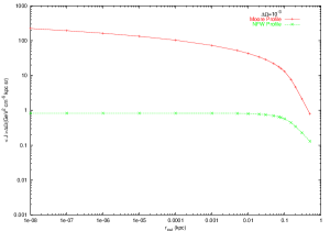
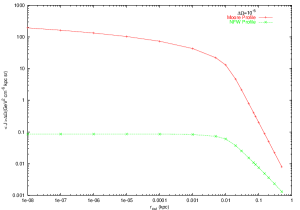
At the position of the Sun, which is about 8.5 kpc away from the the Galactic Center, we can probe the GC to a radius as small as 0.15 kpc (0.015 kpc) using an instrument with the angular resolution of $1^{\circ}$ ($0.1^{\circ}$), corresponding to the solid angle $\Delta\Omega\approx 10^{-3}(10^{-5})$. Therefore we expect the annihilation flux within the solid angle $\Delta\Omega$ will be enhanced greatly if the core radius is smaller than the radius that the instrument can resolve, i.e., $r_{\text{core}}<r_{\text{res}}$. In Fig. 1, we plot the cosmological factor defined as the integration in Eq. (2) as a function of the core radius. From the figure we can see that the cosmological factor increases quickly with decreasing core radius when it is larger than the $r_{\text{res}}$. For smaller $r_{\text{core}}<r_{\text{res}}$, the cosmological factor rises slowly by further decreasing the core radius. This behavior can be understood as below. The flux is proportional to integration of the density square within the solid angle

$$\Phi\sim\int_{0}^{r_{\text{res}}}\rho^{2}(r)r^{2}dr\sim\int_{0}^{r_{\text{core}}}\rho^{2}(r_{\text{core}})r^{2}dr+\int_{r_{\text{core}}}^{r_{\text{res}}}\rho^{2}(r)r^{2}dr\ ,$$ (8)

which gives that the flux in Moore profile depends on $r_{\text{core}}$ logarithmically while independent of $r_{\text{core}}$ for the NFW case.

Figure 1: The cosmological factor within the solid angle $\Delta\Omega$ as function of the core radius for the angular resolution of $\Delta\Omega=10^{-3},\ 10^{-5}$ respectively.

III.1.3 angular resolution

From Eq. (2) we can see that the cosmological factor also depends on the angular resolution of the experimental instruments. We expect a larger cosmological factor for a larger angular resolution which probes greater volume of dark matter annihilation (however, the significance of detection is decreased due to more background is included. see our later discussion). In Fig. 1, we plot the cosmological factor for the solid angular resolution $\Delta\Omega=10^{-3}$ and $\Delta\Omega=10^{-5}$ respectively. For the case when $r_{\text{core}}>r_{\text{res}}$ the cosmological factor for $\Delta\Omega=10^{-3}$ is indeed two orders magnitude larger than that for $\Delta\Omega=10^{-5}$. While for smaller $r_{\text{core}}$ the difference between the two cases is smaller. Especially for the Moore profile the difference is almost negligible.

III.2 Particle factor

We now turn to the particle factor in Eq. (2). We will mainly work in the frame of MSSM, which is a low energy effective description of the fundamental theory at the electroweak scale. For comparison, the minimal supergravity (mSUGRA) model is also explored, where the soft SUSY breaking parameters can be universally defined at the scale of grand unification (GUT). For the R-parity conservative MSSM, the lightest supersymmetric particle (LSP), generally the lightest neutralino, is stable and is an ideal candidate of dark matter.

Even the R-parity conservative MSSM is described by more than one hundred soft supersymmetry breaking parameters. However, for the processes related with dark matter production and annihilation, only several parameters are relevant under some simplifying assumptions, i.e., the higgsino mass parameter $\mu$, the wino mass parameter $M_{2}$, the mass of the CP-odd Higgs boson $m_{A}$, the ratio of the Higgs Vacuum expectation values $\tan\beta$, the scalar quark mass parameter $m_{\tilde{q}}$, the scalar lepton mass parameter $m_{\tilde{l}}$, the trilinear soft breaking parameter $A_{t}$ and $A_{b}$. To determine the low energy spectrum of the SUSY particles and coupling vertices, the following assumptions have been made: all the sleptons and the squarks have common soft-breaking mass parameters $m_{\tilde{l}}$ and $m_{\tilde{q}}$ respectively; all trilinear parameters are zero except those of the third family; the bino and wino have the mass relation, $M_{1}=5/3\tan^{2}\theta_{W}M_{2}$, coming from the unification of the gaugino mass at the grand unification scale.

We perform a numerical random scanning of the 8-dimensional supersymmetric parameter space using the package DarkSUSY darksusy . The ranges of the parameters are as following: $50GeV<|\mu|,\ M_{2},\ M_{A},\ m_{\tilde{q}},\ m_{\tilde{l}}<5TeV$, $1.1<\tan\beta<55$, $-3m_{\tilde{q}}<A_{t},\ A_{b}<3m_{\tilde{q}}$, $\text{sign}(\mu)=\pm 1$. The parameter space is constrained by the theoretical consistency requirement, such as the correct vacuum breaking pattern, the neutralino being the LSP and so on. The accelerator data constrains the parameter further from the spectrum requirement, the invisible Z-boson width, the branching ratio of $b\to s\gamma$ and so on adopting the 2002 limits of the Particle Data Grouppdg .

Another important constraint comes from cosmology. Combining the recent observation data on cosmic microwave background, large scale structure, supernova and data from HST Key Project the cosmological parameters are determined quite precisely. Especially, the abundance of the cold dark matter is given by wmap $\Omega_{\text{CDM}}h^{2}=0.113^{+0.008}_{-0.009}$. We constrain the SUSY parameter space by requiring the relic abundance of neutralino $0<\Omega_{\chi}h^{2}<0.137$, where the upper limit corresponds to the 3$\sigma$ upper bound from the cosmological observations. When the relic abundance of neutralino is smaller than a minimal value the neutralino represents a subdominant dark matter component. We then rescale the galaxy dark matter density as $\rho(r)\to\xi\rho(r)$ with $\xi=\Omega_{\chi}h^{2}/(\Omega_{\chi}h^{2})_{\text{min}}$. We take $(\Omega_{\chi}h^{2})_{\text{min}}=0.086$, the 3$\sigma$ lower bound of the CDM abundance wmap . The effect of coannihilation between the fermions is taken into account when calculating the relic density numerically.

Besides exploring the SUSY parameter space at low energy directly under some simplifying assumptions, there is another popular approach of handling the phenomenology of MSSM by assuming a simple SUSY breaking pattern at the GUT scale. One of the simplest models in this kind is the minimal supergravity model which has only five free SUSY parameters, the gaugino masses $m_{1/2}$, the sfermion masses $m_{0}$, the trilinear parameter $A_{0}$, which are all defined universally at the GUT scale, as well as the ratio of the vacuum expectation values $\tan\beta$ and the sign of the higgino mass parameter $\mu$. The high energy universal relationship leads to constraints on the low energy spectrum ellis . To calculate the neutralino annihilation, we adopt the package ISASUGRA (version 7.69) to calculate the low energy SUSY spectrum by numerical solving the renormalization group equations from the GUT scale downwards to the weak scale isajet . We also randomly scan the free parameter space considering the theoretical and experimental constraints. The ranges of the parameters are given as $50GeV<m_{0},m_{1/2}<5TeV$, $-3m_{0}<A_{0}<3m_{0}$, $1.1<\tan\beta<55$ and $\text{sign}(\mu)=\pm 1$.

The $\gamma$-rays from the neutralino annihilation arise mainly in the decay of the neutral pions produced in the fragmentation processes initiated by tree level final states. The fragmentation and decay processes are simulated with Pythia packagepythia incorporated in DarkSUSY. We focus our calculation on the continuum $\gamma$-rays from the pion decays.

III.2.1 constraints from cosmic ray observations

Before presenting the numerical results we discuss the constraints from the cosmic ray observations first. High energy and very high energy $\gamma$-ray emission from the GC have been detected by the EGRET egret , CANGAROO-II cang and HESS hess experiments. However, the present situation is still confused since all these results can not be attributed to a unique $\gamma$-ray source or due to a single emission mechanism. Therefore we take all these results as a constraint on the dark matter annihilation, i.e., the predicted $\gamma$-rays flux due to the DM annihilation should not exceed these observed fluxes.

The $\gamma$-ray spectrum from the EGRET observationegret at the GC with the angular resolution of $\sim 1^{\circ}$ is well described by a broken power law with a break energy at $1.9GeV$. Above this energy the photon spectrum is $F(E)=1.6\times 10^{-6}(E/GeV)^{-3.1}cm^{-2}s^{-1}GeV^{-1}$. Assuming that this spectrum can extend to a quite high energy we get an approximate integrated $\gamma$-ray flux above $1GeV$ using this power spectrum $F(E>1GeV)=7.7\times 10^{-7}cm^{-2}s^{-1}$.

Both CANGAROO-II and HESS observed $\gamma$-rays at the GC from about $200GeV$ to about $10TeV$. The HESS data hess is fitted by a power law spectrum $F(E)=2.5\times 10^{-12}(E/TeV)^{-2.21}cm^{-2}s^{-1}TeV^{-1}$. The CANGAROO-II cang ; Hooper gives a quite different power law spectrum with a spectral index $-4.6$. The apparent discrepancy seems indicate a significant change of the source at lower energies over about one year. However, none of the individual experiment observes significant variability of the source. Another possible explanation is that due to larger positional uncertainty of the CANGAROO-II there may be more than one source exist in the direction of the GChorns . The flux detected by HESS is also much lower than that detected by EGRET if extending the spectrum to lower energies. Therefore we take a relaxed constraint from the HESS experiment, which has the best angular resolution of $0.1^{\circ}$: assuming that the source at the GC can extend to the range within an angular resolution of $1^{\circ}$, despite a point-like source can fit the single HESS observation wellhess . We then get the integrated flux above $100GeV$ using the given spectrum $F(E>100GeV)=3.4\times 10^{-9}cm^{-2}s^{-1}$. The integrated flux from the CANGAROO-II data by extending its spectrum to lower energy, $F(E>100GeV)=2.8\times 10^{-9}cm^{-2}s^{-1}$. Anyway, at the moment the situation is not clear we take these values as a conservative constraints so that we can probe more SUSY parameter space. For further more severe constraints more SUSY parameter space will be constrained and our later results can be simply rescaled due to Eq. (2).

III.3 Results

Figure 2: The integrated $\gamma$-ray fluxes from neutralino annihilation at the GC above the threshold energy of $1$, $10$, $50$, $100$ and $1000$ GeV respectively for the Moore (upper panel) and the NFW (lower panel) profiles as function of the neutralino mass. The fluxes are given within the angular resolution of $\Delta\Omega=10^{-3}$. Each dot in the figure represents a set of low energy SUSY parameters which survive all the current limits. The bigger points superposed on each set of dots (corresponding to a threshold energy) are given by the mSUGRA model.

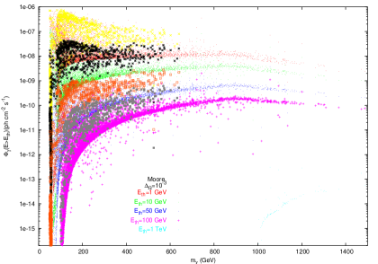
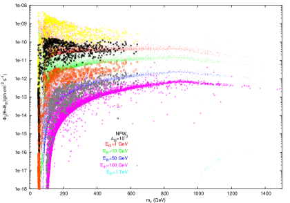
Combining all these constraints together, from the theoretical consideration to the accelerator experiments and cosmic ray observations, we can give the predicted $\gamma$-ray fluxes from neutralino annihilations at the GC now. In Fig. 2, we plot the integrated $\gamma$-ray fluxes within the solid angle $\Delta\Omega=10^{-3}$ as a function of the neutralino mass taking the threshold energy as $1GeV$, $10GeV$, $50GeV$, $100GeV$ and $1TeV$ for both the Moore and the NFW profiles. Each dot in the figure corresponds to a model with a set of definite SUSY parameters in the 8-dimensional parameter space allowed by all the constraints. The bigger points superposed on each set of dots are given by the mSUGRA model. We notice that the mSUGRA model tends to give large annihilation fluxes, while small neutralino mass which is hard to be greater than $800GeV$. The scatter of the points represents the uncertainty coming from the unknown soft SUSY breaking parameters.

It is worth giving some comments here. First, the core radius is taken as $10^{-8}$ kpc for both the Moore and the NFW profiles. From Fig. 1 we can see that the flux in the Moore profile decrease only by a factor of 2 when taking $r_{\text{core}}$ from $10^{-8}$ kpc to $10^{-4}$ kpc. For the case of NFW profile the predicted flux has no change even taking $r_{\text{core}}$ as large as $0.1$ kpc. Second, in the case of Moore profile the SUSY parameter space has been constrained by the cosmic ray observations at the GC. If more stringent constraints are adopted all the later results according to the Moore profile will be rescaled. However, there is no constraints for the case of the NFW profile. Third, except the region near the threshold energy the uncertainties of the predicted $\gamma$-ray fluxes are within two orders of magnitude even scanning the 8-dimensional parameter space which spans quite a large range, as given in the last subsection. The most strong constraint comes from the requirement by cosmology, i.e., requiring $0<\Omega_{\text{CDM}}h^{2}<0.137$. For s-wave annihilation the rate $\langle\sigma v\rangle_{\text{ann}}$ is closely related with the initial value of $\langle\sigma v\rangle_{\text{ini}}$ at the decoupling epoch which determines the relic density of neutralino. Forth, the neutralino mass above $1\ TeV$ is difficult to achieve after taking all the constraints into account. We can realize a model with the neutralino mass at most as heavy as about $5\ TeV$ to satisfy all the constraints after we relax the range of all low energy soft mass parameters as large as $50TeV$. Therefore, a neutralino as heavy as $18\ TeV$ to explain the spectrum observed by HESS experiment horns ; profumo ; Ferrer as neutralino annihilation will be very hard to achieve in the framework of MSSM.

For discussions of the substructure emission in the next sections we will fix the ‘particle factor’ by taking an optimistic set of SUSY parameters. The ‘particle factor’ is such taken that the integrated $\gamma$-ray fluxes above $100GeV$ from the GC for the Moore profile is $F(E>100GeV)=10^{-9}cm^{-2}s^{-1}$, which is near the maximal value of the SUSY prediction. This is just a normalization of the $\gamma$-ray flux and only the relative magnitude of the fluxes between the GC and the substructure is relevant, since the overall magnitude can be rescaled according to different particle factors.

We can summarize this section here. By scanning the SUSY parameter space and after taking all the constraints into account we give the scatter of the integrated $\gamma$-ray fluxes from neutralino annihilations at the GC in Fig. 2 for different threshold energies and for both the Moore and the NFW profiles. From the factorization of the expression in Eq. (2) we know this figure is suitable to any other source by multiplying each point by a global factor which represents the difference of the ‘cosmological factor’ from that at the GC. Therefore the figure shows the general uncertainties of the particle factor. The uncertainty is quite small considering the huge volume of the free parameter space. This is due to the fact that the annihilation process is closely related with the process of dark matter freezing out which determines its relic density.

IV Gamma rays from the subhalos

IV.1 realization of MW with substructures

To predict the $\gamma$-ray flux by neutralino annihilation from the subhalos we need to know the distribution of subhalos in the MW and the density profile within each subhalo.

The properties of subhalos are determined via the competition between accretion and destruction due to tidal force and dynamical friction. N-body simulation and semi-analytical methods have been extensively used to investigate the spatial distribution and mass function of substructures in the host halo. According to the extensive studies it is now believed that the radial distribution of substructures is generally shallower than density profile of the smooth background. The reason for the anti-bias of the substructure number density relative to the smooth distribution is due to the tidal disruption of substructures which is most effective near the galactic center. This conclusion does not depend on the numerical resolution as confirmed in Ref. diemand by adopting a wide range of mass and force resolutions. It is shown that the relative number density of subhalos can be approximated by an isothermal profile with a core diemand

$$n(r)=2n_{H}(1+(r/r_{H})^{2})^{-1}\ ,$$ (9)

where $n_{H}$ is the relative number density at the scale radius $r_{H}$. The average core radius for the distribution of galaxy subhalos is about $0.14$ times the halo virial radius, $r_{H}=0.14r_{\text{vir}}$. The core radius is a smaller fraction of the virial radius than that of cluster subhalosdiemand , since galaxy forms earlier and is more centrally concentrated. The spatial distribution given above agrees well with that in another recent simulation by Gao et al. gao .

At large radius $n(r)$ in Eq. (9) goes as $r^{-2}$ which represents the anti-bias since the DM profile goes as $r^{-3}$ at large radius for both the NFW and the Moore profiles. It is worth mentioning that most previous works calculating $\gamma$-rays from substructures adopting a fitted formula given in Ref. blasi , $n(r)\propto(1+(r/r_{H})^{2})^{-1.5}$, which follows the DM profile and does not reflect the anti-bias of the substructure distribution.

Simulations show that the differential mass function of substructures has an approximate power law distribution, $dn/dm\sim m^{-\alpha}$, with no dependence or slight dependence on the host halo mass. Most studies point out that the cluster and galaxy have similar substructure mass function although the clusters form much later than galaxies in the hierarchical structure formation scenario. It seems that the tidal effects change the mass distribution function self-similarly. In Ref. diemand both the cluster and galaxy substructure cumulative mass functions are found to be an $m^{-1}$ power law, $n_{\text{sub}}(m_{\text{sub}}>m)\propto m^{-1}$, with no dependence on the mass of the parent halo. A slight difference is found in a recent simulation by Gao et al. gao that the cluster substructure is more abundant than galaxy substructure since the cluster forms later and more substructures have survived the tidal disruption. The mass function for both scales are well fitted by $dn/dm\propto m^{-1.9}$. A non-universal form of the mass function is found in Ref. ghigna00 : the power index of the cumulative mass function is $-1$ for $m_{\text{sub}}>10^{11}h^{-1}M_{\odot}$ while it changes to $-0.7$ for $m_{\text{sub}}<10^{11}h^{-1}M_{\odot}$. There is an advantage of a power law form for the differential mass function shallower than $m^{-2}$: the fraction of the total mass enclosed in subhalos is then insensitive to the mass of the minimal subhalo we take. The mass fraction of subhalos estimated in the literature is around between 5 percent to 20 percent ghigna00 ; springel01 ; stoehr . In this work we will always take the mass fraction of substructures as 10 percent.

Putting all these arguments together, we get the probability of a substructure with mass $m$ at the position $r$ to the galactic center

$$n(m,r)=n_{0}\left(\frac{m}{M_{\text{vir}}}\right)^{-1.9}(1+(r/r_{H})^{2})^{-1}\ ,$$ (10)

where $M_{\text{vir}}$ is the virial mass of the MW, $n_{0}$ is the normalization factor determined by requiring the total mass of substructures converges to 10 percent of the MW virial mass, $M_{\text{vir}}$. A population of substructures within the virial radius of the MW are then realized statistically due to Eq. (10). The mass of the substructures are taken randomly between $M_{\text{min}}=10^{6}M_{\odot}$, which is the lowest substructure mass the present simulations can resolve cut , and the maximal mass $M_{\text{max}}$. The maximal mass of substructures is taken to be $0.01M_{\text{vir}}$ since the MW halo does not show recent mergers of satellites with masses larger then $\sim 2\times 10^{10}M_{\odot}$. It will be shown that the $\gamma$-ray flux is quite insensitive to the minimum subhalo mass since the flux from a single subhalo scales as its mass kou ; aloisio .

We notice that the number density of substructures is largest at the GC due to Eq. (10) which, however, is in conflict with the fact that most substructures near the GC are destroyed by the strong tidal effect. The underestimate of the tidal effect near the GC in Eq. (10) is due to the finite resolution of the N-body simulations and the formula is an extrapolation of the subhalo distribution to smaller radius. The global tides from the host halos strip outer parts of the substructures and result in the substructure disruption or at least significant amount of substructure mass loss. We take the tidal effects into account under the “tidal approximation”, which assumes that all mass beyond a suitably defined tidal radius is lost in a single orbit while keep its density profile inside the tidal radius intact.

The tidal radius is defined as the radius of the substructure at which the tidal forces of the host exceeds the self gravity of the substructure. Assuming that both the host and the substructure gravitational potential are given by point masses and considering the centrifugal force experienced by the substructure the tidal radius at the Jacobi limit is given by hayashi

$$r_{\text{tid}}=r_{c}\left(\frac{m}{3M_{vir}}\right)^{\frac{1}{3}}\ ,$$ (11)

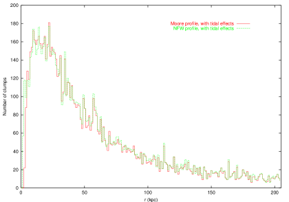
where $r_{c}$ is the distance of the substructure to the GC. The substructures with $r_{\text{tid}}\lesssim r_{s}$ will be disrupted completely and be discarded in our realization of the substructure population. The mass of a substructure is also recalculated by subtracting the mass beyond the tidal radius. Therefore the final radial distribution of substructures near the GC is somewhat different from that given in Eq. (10) which is shown in Fig. 3. Indeed the substructures near the GC are disrupted completely after we take the tidal effects into account. The substructures with NFW profile can exist more near the GC than the Moore profile. This is because that the NFW profile is more centrally concentrated with smaller $r_{s}$.

Figure 3: Number of substructures along the radius of the MW for the Moore and the NFW profiles.

IV.2 Concentration parameter

Once the population of the substructures are determined we need to determine the dark matter density profile in each substructure in order to calculate the annihilation of neutralinos. The density profile in the substructure, either the NFW or the Moore profile, is characterized by two scale parameters $\rho_{s}$ and $r_{s}$. The two parameters can be determined using two different methods. In the first method they are determined by one virial parameter, the virial mass (or equivalently the virial radius, or virial velocity), and the concentration parameter, which relates the virial and the inner scale radius.

N-body simulation shows that the concentration of the substructure is strongly correlated with the formation epoch of the substructure. At an epoch of redshift $z_{c}$ a typical collapsing mass $M_{*}(z_{c})$ is defined by $\sigma[M_{*}(z)]=\delta_{sc}(z)$, where the $\sigma[M_{*}(z)]$ is the linear rms density fluctuation on the comoving scale encompassing a mass $M_{*}$, $\delta_{sc}$ is the critical overdensity for collapsing at the spherical collapse model. The collapsing mass $M_{*}$ is determined by the primordial linear power spectrum of the fluctuations and the known cosmology, which determines the evolution of the fluctuations. In a semi-analytic model Bullock et al.bullock01 relate the typical collapsing mass to a fixed fraction of the virial mass of a halo $M_{*}(z_{c})=FM_{\text{vir}}$. The concentration parameter of a halo with virial mass $M_{\text{vir}}$ at redshift $z$ is then determined as $c_{\text{vir}}(M_{\text{vir}},z)=K\frac{1+z_{c}}{1+z}$. Both $F$ and $K$ are constants to fit the numerical simulations. Once $F$ and $K$ are determined the concentration of a halo is completely determined by the cosmology in hand. We notice that a smaller $M_{\text{vir}}$ corresponds to a smaller collapsing mass and early collapsing epoch when the Universe is denser and therefore a larger concentration parameter. Therefore smaller subhalos are more closely concentrated.

Figure 4: Concentration parameter as a function of the virial mass of the halo calculated according to the Bullock modelbullock01 . The model parameters are taken as $F=0.015$ and $K=4.4$. The cosmology parameters are taken as $\Omega_{M}=0.3$, $\Omega_{\Lambda}=0.7$, $\Omega_{B}h^{2}=0.02$, $h=0.7$, $\sigma_{8}=0.9$ with three generations of massless neutrinos.

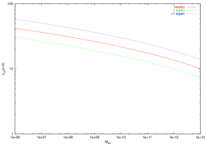
In Fig. 4 we plot the concentration parameter at $z=0$ as a function of the virial mass of a halo according to the Bullock modelbullock01 . In the calculation, we have taken a standard scale invariant primordial spectrum of the fluctuation with the cosmology parameters taken as $\Omega_{M}=0.3$, $\Omega_{\Lambda}=0.7$, $\Omega_{B}h^{2}=0.02$, $h=0.7$, $\sigma_{8}=0.9$ and three generations of massless neutrinos. The model parameters are taken as $F=0.015$ and $K=4.4$. The scatter of the concentration parameters for a given halo mass is log-normal with $1\sigma$ deviation around the mean as $\Delta(\log_{10}c_{\text{vir}})=0.14$. In Fig. 4 both the median and the $\pm 1\sigma$ values of the concentration parameters are plotted.

The Bullock model reproduces the concentration parameters quite well from the N-body simulations. From Fig. 4 the experiential formula is confirmed again that $c_{\text{vir}}\propto M_{\text{vir}}^{-\beta}$. We expect that this exponential relation of the concentration parameter and virial mass for subhalos should be very well followed, since subhalo forms early at the epoch when the Universe is dominated by matter with approximate power-law power spectrum of fluctuations. Besides the Bullock model we have also adopted other recent simulation results in the literature. We use the experiential relation between the concentration parameters and virial mass and fit the parameter $\beta$ from these simulation results. The density profile of the substructure and furthermore the $\gamma$-ray flux from the substructure are then calculated. We find the concentration parameter is the most sensitive parameter in determining the $\gamma$-ray flux. Different behavior of the concentration leads to different predictions of the $\gamma$-ray fluxes.

The second method to determine the profile parameters, as given in tasit , requires each substructure produced following Eq. (10) is compact enough to resist the tidal stripping. Since the distribution of substructures in Eq. (10) is given by simulations at $z=0$ the second method reflect the simulation results faithfully in the statistical meaning. Since the simulation can not resolve the region near the GC we have given a cutoff at $r=10$ kpc from the GC requiring no subhalo exits inside the cutoff radius. The conditions to determine the parameters are given bytasit : $R_{\text{vir}}=R_{\text{tid}}$, $\int_{0}^{R_{\text{vir}}}\rho(r)dV=M_{sub}$ and $\rho_{host}(r_{cl})=\rho_{cl}(R_{\text{vir}})$. The last condition requires that the density of the subhalos at $R_{vir}$ should equal the local density of the host halo at the position of the subhalo $r_{cl}$.

IV.3 Results

Figure 5: The integrated $\gamma$-ray fluxes above $100GeV$ as function of the angles of the sources relative to the GC. In the upper panel we adopt the concentration parameters of the subhalos given in bullock01 while in the lower panel we adopt that in reed . Both contributions from the smooth component of DM and from subhalos are plotted.

We can now present the results of the $\gamma$-ray fluxes from the neutralino annihilation in the MW substructures. The fluxes are averaged within the angular resolution of $1^{\circ}$ in the following way: if a subhalo is too small or too far from the detector that its angular size is smaller than the angular resolution we calculate the annihilation flux of the whole subhalo; on the contrary for these subhalos the detector can resolve we calculated the flux within the $1^{\circ}$ angular resolution assuming that we are aiming at the center of the subhalo. The annihilation core radius in the following calculations is taken as $r_{cut}=10^{-4}kpc$, which is quite a conservative value and affects the the results little according to Fig. 1.

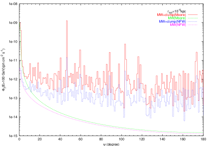
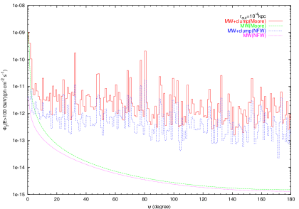
In Fig. 5 we plot the integrated $\gamma$-ray fluxes above the threshold energy of 100 GeV as a function of $\psi$, the angle of the source to the direction of the GC. In the figure no information is shown about the other direction around the axis along the Sun and the GC. Only the maximal $\gamma$-ray flux at this direction is chosen for each $\psi$ and plotted in the figure. Both the $\gamma$-rays annihilated from the smooth dark halo and that by adding the emission from the subhalos and the smooth component are shown for the Moore and the NFW profiles. For the smooth component the $\gamma$-ray flux decreases rapidly when departing from the GC while for the subhalos the contribution seems almost isotropic to different directions. This is due to the fact that the Sun is only $8.5$ kpc away from the GC. In the upper panel we calculate the flux adopting the Bullock modelbullock01 and in the lower panel we adopt the concentration parameter according to the simulation by Reed et al. reed . Generally the Moore profile predicts greater $\gamma$-ray fluxes. At the GC the $\gamma$-ray flux for the Moore profile is about 300 times higher than that for the NFW profile. However, for the subhalos the difference between the two profiles is only about one order of magnitude. Therefore the uncertainty of the predicted $\gamma$-ray fluxes from the subhalos due to the cosmological factor is much smaller than that from the GC. The figure can be used to other threshold energies by a global shift of the particle factor from the Fig. 2.

Figure 6: The cumulative number of subhalos as function of the integrated $\gamma$-ray fluxes $n(>\Phi_{\gamma})$ for the Moore profile (upper panel) and the NFW profile (lower panel). The results are given within the zenith angle of $60^{\circ}$. The curves represent the results according to different simulations as explained in the text. These curves give the number of subhalos which emit $\gamma$-rays with the integrated flux above $\Phi_{\gamma}$.

It should be noted that Fig. 5 illustrates the $\gamma$-ray fluxes from the subhalos due to a statistical realization of our Galaxy. None of the positions of peaks are predicted exactly and the maximal flux may have a large fluctuation: it is possible that a subhalo is accidentally located near the solar system. Therefore we try to calculate the statistically averaged fluxes by realizing one hundred MW sized halos and count the average number of subhalos emitting $\gamma$-rays above any intensities.

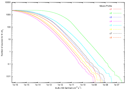
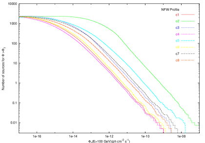
Fig. 6 gives the cumulative number of subhalos emitting $\gamma$-rays with intensity above the integrated flux $\Phi_{\gamma}$. It should be noted that the results, also for other figures hereafter, are given within the zenith angle of $60^{\circ}$, which is the maximal angle a ground array can possibly probe, instead of the whole sky. In the upper panel we plot the results for the Moore profile while the lower panel is for the NFW profile. The curves are given by calculating the density profile of subhalos according to different author’s simulation results, where ‘c1’ denotes the simulation of Ref. klypin ; ‘c3’ of Ref. reed ; ‘c4’ of Ref. eke for the $\Lambda$CDM model with $\sigma_{8}=0.9$; ‘c6’ uses the median $c_{vir}-M_{vir}$ relation for distinct halos of the Bullock model given in Ref. bullock01 , while ‘c7’ and ‘c8’ take the upper $2\sigma$ and $1\sigma$ values of the same model respectively; ‘c2’ adopts the simulation results given in dense matter environment of the same reference and extends the relation to small subhalos; since this relation gives very large concentration parameters for small subhalos we have cut the concentration parameter arbitrarily if $c>100$ in ‘c5’. From this figure we can easily read the number of the expected detectable subhalos if the sensitivity of a detector is given (with same threshold energy and angular resolution adopted here).

Figure 7: The cumulative number of subhalos as function of the integrated $\gamma$-ray fluxes $n(>\Phi_{\gamma})$ for the Moore profile (upper panel) and the NFW profile (lower panel). The results are given within the zenith angle of $60^{\circ}$. The lines are the corresponding fits of the curves for high $\gamma$-ray fluxes. From these fits we can easily read out the number of subhalos which emit $\gamma$-rays with the integrated flux above $\Phi_{\gamma}$.

Figure 8: The cumulative number of subhalos as function of the integrated $\gamma$-ray fluxes $n(>\Phi_{\gamma})$ for taking different cuts of the minimal mass of the subhalos. The results are given within the zenith angle of $60^{\circ}$. The lines are the corresponding fits of the curves for high $\gamma$-ray fluxes. The results are quite insensitive to the cut of the minimal subhalo mass.

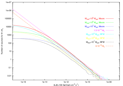
	c1	c2	c3	c4	c5	c6	c7	c8
Moore	$1.5\times 10^{-11}$	$2\times 10^{-9}$	$6\times 10^{-11}$	$8\times 10^{-12}$	$3\times 10^{-10}$	$2\times 10^{-11}$	$8\times 10^{-11}$	$4\times 10^{-11}$
NFW	$4.5\times 10^{-12}$	$7\times 10^{-10}$	$2\times 10^{-11}$	$3.5\times 10^{-12}$	$9\times 10^{-11}$	$6\times 10^{-12}$	$3\times 10^{-11}$	$1.5\times 10^{-11}$

Table 1: Values of the constant $n_{0}$ in the fit $n(>\Phi_{\gamma})=n_{0}/\Phi_{\gamma}$ to the curves in Fig. 6 for the Moore and the NFW profiles.

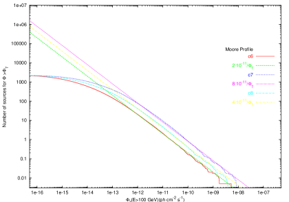
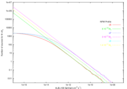
We find the cumulative number of subhalos for large fluxes can be well fitted by an inverse power law, $n(>\Phi_{\gamma})=n_{0}/\Phi_{\gamma}$, as shown in Fig. 7. The deviation of the calculated curves from the fitted lines at the end of largest fluxes is due to the fact that we do not have enough statistics here, while the deviation at the end of lowest fluxes may be due to the cut of the minimal mass of subhalos. In the table 1 we give the fitted constant $n_{0}$ for different curves. The Moore profile predicts about 3 times more detectable subhalos than the NFW profile averagely. Therefore the $\gamma$-ray fluxes from the subhalos are not so sensitive to the dark matter profiles as these from the GC, as shown in the Fig. 5. In Fig. 8 we show how the cumulative number of subhalos changes as the value we take for the minimal mass of subhalo. We illustrate the result in the model ‘c1’. The dependence on the minimal mass of subhalo is very weak, which can be understood from some simple scaling argumentskou . It is worth noting that taking smaller minimal subhalo mass indeed makes the curves closer to the fitted lines at the end of smallest fluxes.

Figure 9: The cumulative number of subhalos as function of the integrated $\gamma$-ray fluxes $n(>\Phi_{\gamma})$. The results are given within the zenith angle of $60^{\circ}$. The curves are calculated according to the second method to determine the profile parameters as described in the text. The corresponding results from the models ‘c2’ and ‘c6’ are also shown.

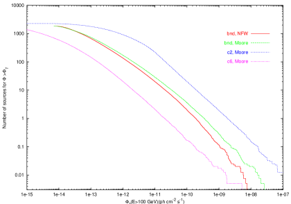
Finally, in Fig. 9 we give the results according to the second method of determining the concentration parameter. Both the NFW and Moore profiles predicts much larger fluxes compared with that from the model ‘c6’ using the Moore profile, while smaller than that of the ‘c2’ model.

In summary, we calculated the $\gamma$-ray fluxes from the MW substructures in this section. There are extensive studies on the evolution and distribution of substructures by numerical simulations. We integrate the recent simulation results in our calculation. The different simulation results give uncertainties in predicting the $\gamma$-ray fluxes. The concentration parameter is the most sensitive parameter in determining the $\gamma$-ray fluxes. We give the statistical average number of subhalos with $\gamma$-ray intensity above some values. The result is well fitted by an inverse power law. From these results the number of detectable subhalos is easily read out if the sensitivity of a detector is known. We will discuss the detectability of the $\gamma$-ray signals from the MW subhalos in the next section.

V detectability

The detectability of a signal is defined by the ratio of the signal events to the fluctuation of the background. Since the background follows the Poisson statistics, its fluctuation has the amplitude proportional to $\sqrt{N_{B}}$. The significance of the detection is quantified by $\sigma=\frac{n_{\gamma}}{\sqrt{N_{B}}}$.

The signal events are given by

$$n_{\gamma}=\epsilon_{\Delta\Omega}\int_{E_{th},\Delta\Omega}A_{eff}(E,\theta)\phi(E)dEd\Omega dT\ \ ,$$ (12)

where $\epsilon_{\Delta\Omega}=0.68$ is the fraction of signal events within the angular resolution of the instrument and the integration is for the energies above the threshold energy $E_{th}$, within the angular resolution of the instrument $\Delta\Omega$ and for the observational time. The effective area $A_{eff}$ is a function of energy and zenith angle. The $\phi(E)$ is the flux of $\gamma$-rays from DM annihilation.

The corresponding expression for the background is similar to Eq. (12). The background includes contributions from the hadronic and electronic comic-rays and the Galactic and extragalactic $\gamma$-ray emission. We have adopted the expressions as

$$\phi_{h}(E)=1.49E^{-2.74}cm^{-2}s^{-1}sr^{-1}GeV^{-1}$$ (13)

for the hadronic contribution gaisser ,

$$\phi_{e}(E)=6.9\times 10^{-2}E^{-3.3}cm^{-2}s^{-1}sr^{-1}GeV^{-1}$$ (14)

for the electronic contribution longair ,

$$\phi_{\text{extra}-\gamma}(E)=1.38\times 10^{-6}E^{-2.1}cm^{-2}s^{-1}sr^{-1}GeV^{-1}$$ (15)

for the extragalactic $\gamma$-ray emission extrapolated from EGRET data at low energiesextra and

$$\phi_{\text{galac}-\gamma}(E)=N_{0}(l,b)\times 10^{-6}E^{-2.7}cm^{-2}s^{-1}sr^{-1}GeV^{-1}$$ (16)

for the Galactic $\gamma$-ray emission, also extrapolated from the EGRET data at low energiesgal , with $N_{0}$ the normalization factor depending on galactic coordinates $(l,b)$. The $N_{0}$ is modeled using EGRET data at 1 GeV gal

$$N_{0}(l,b)=\frac{85.5}{\sqrt{1+\left(l/35\right)^{2}}\;\sqrt{1+\left(b/(1.1+|l|\,0.022)\right)^{2}}}\,+\,0.5$$ (17)

for $|l|\,\geq 30^{\circ}$ and

$$N_{0}(l,b)=\frac{85.5}{\sqrt{1+\left(l/35\right)^{2}}\;\sqrt{1+\left(b/1.8\right)^{2}}}\,+\,0.5$$ (18)

for $|l|\,\leq 30^{\circ}$, with the longitude $l$ and the latitude $b$ varying in the intervals $[-180^{\circ},180^{\circ}]$ and $[-90^{\circ},90^{\circ}]$, respectively.

Since most background comes from the hadronic cosmic rays, the hadron-photon identification efficiency is an important factor to reduce the physical background. For a satellite borne experiments, such as GLAST glast , an identification efficiency of charged particles as high as $99.997\%$ can be assumed, while $90\%$ for the photonsgeff . However, the effective area of this kind of experiments is limited by the size of the satellite and has the order of $A_{eff}\sim 1m^{2}$. The atmospheric Čerenkov telescopes (ACT), such as VERITASveritas , MAGICmagic and HESShessh , can have very large effective area with an identification efficiency of $99\%$ for both the hadronic and the electromagnetic primary particles. However, the ACTs have a small field of view ($\sim 5^{\circ}$) with a duty cycle of about 10%. Therefore the ACTs are suitable for the observation of point sources and can not do the blind search.

The ground-based extensive air shower (EAS) arrays, such as ARGOargo , MILAGROmilagro and the next generation all-sky high energy $\gamma$-ray telescope HAWChawc , have complementary properties to the satellite borne experiments and the ACTs. They also have large effective areas and at the same time they have large filed of view ($\sim 60^{\circ}$) and a duty cycle of about 100%. However, the EAS arrays have low hadron-photon identification efficiency. For the ARGO we assume no discrimination between the hadron and the photon, while for the HAWC the hadron-photon discrimination can improve the significance of the detection by a quality factor of 1.6 hawc .

Figure 10: The $3\sigma$ sensitivity curves of different detectors as functions of the threshold energy of the $\gamma$-rays. The curves are calculated according to the parameters given in the text.

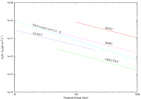
In Fig. 10 we show the $3\sigma$ sensitivity curves of different detectors as function of the threshold energy. We have assumed the angular resolution as $0.1^{\circ}$ for GLAST and VERITAS and the angular resolution as $1^{\circ}$ for ARGO and HAWC. For GLAST, ARGO and HAWC we use 1 year of data taking, while for VERITAS 250 hours observation pointing to a source is assumed. We make rough approximation of energy independent effective area, $10^{3}m^{2}$, $3\times 10^{4}m^{2}$ and $4\times 10^{4}m^{2}$ for ARGO, HAWC and VERITAS respectively. The diffuse extragalactic $\gamma$-ray background from Eq. (15) is also plotted in the figure for comparison.

The detectability of GLAST and VERITAS for the $\gamma$-rays from the Galactic subhalos has been carefully studied in the Ref. kou ; peirani . It is shown that the significance of the detection of the annihilated $\gamma$-rays at GLAST is maximized for $M_{\chi}\approx 40GeV$, since GLAST has low energy threshold and thus introduces large background and the $\gamma$-ray flux decreases when increasing the neutralino mass. For neutralino heavier than $100GeV$ GLAST has little chance to detect the signalkou . We can get similar conclusion from Fig. 2 that for small threshold energy the maximal flux is at the lower end of the neutralino mass while as the threshold energy becomes higher the position of the maximal flux moves to a neutralino mass of several hundred GeV. VERITAS, with a higher threshold energy, is sensitive enough to detect the $\gamma$-rays annihilated from heavy neutralinos. However, its small field of view limits its ability to do such observationkou .

However, it is possible to do the observation by the EAS array according to our calculations. Taking the threshold energy as $100GeV$, ARGO and HAWC require the $\gamma$-ray fluxes as high as $8\times 10^{-11}cm^{-2}s^{-1}$ and $1\times 10^{-11}cm^{-2}s^{-1}$, respectively, to achieve a $3\sigma$ significance detection. Comparing with the Table I, we get that ARGO can detect 0.1 to as many as about 25 subhalos with a Moore profile and from 0.04 to about 9 subhalos with a NFW profile for one year data taking. For HAWC, since its sensitivity is about 8 times higher than that of ARGO it can also detect more subhalos by 8 times than that of ARGO. For example, for the Bullock model and its $2\sigma$ upper limit, ARGO has the ability to detect $1/4$ and $1$ subhalos respectively for the Moore profile and about $0.1$ to $0.4$ subhalos respectively for the NFW profile. While for HAWC even with NFW profile and the median concentration parameter of the Bullock model it can detect about $1$ subhalo for one year observation.

Here we can conclude that for the neutralino dark matter as light as about $100GeV$ GLAST is most suitable to observe the annihilated $\gamma$-rays from the Galactic subhalos. For the heavier neutralino dark matter $\sim 500GeV$ ($<1TeV$) ARGO/HAWC can be a viable complementary. Especially, if HAWC is built it has great potential to do the observation.

VI discussion and conclusions

In this work we calculated the $\gamma$-ray fluxes produced by the dark matter annihilation in the Galactic subhalos and discussed the detectability of such signals by different types of detectors according the nature of the dark matter.

We explored the low energy parameter space of the MSSM and studied the uncertainties from the particle physics in predicting the $\gamma$-ray fluxes. Uncertainties from the astrophysics are also carefully studied, where we find the most sensitive parameter in predicting the $\gamma$-ray fluxes is the concentration parameter of subhalos. At the moment there exist discrepancies according to different author’s numerical simulations. We present the results according to several recent simulation results.

Assuming optimistic SUSY parameters the $\gamma$-rays from subhalos may be detected by satellite borne experiment, such as GLAST, which has large field of view and small effective area if the $\gamma$-ray flux is large enough kou (when the neutralino is light $\lesssim 100GeV$). On the contrary, when the neutralino mass is large ($\sim 500GeV$) the $\gamma$-ray flux is reduced and only ground based experiments with large effective area and large field of view, such as ARGO/HAWC, can do the job. We calculated the statistic average numbers of the detectable subhalos at these detectors.

If such an annihilation signal is indeed detected in the future it will not only indicate the weakly interaction between the dark matter particles and further implicate the nature of new physics beyond the SM but also tell us a lot about the nature of the subhalos: they must have a cuspy profile with the Moore or the NFW form or some form between them and the CDM scenario is favored without power suppression at the subgalactic scale. However, from this single measurement neither the SUSY parameter space nor the subhalos distribution and its profile can be actually determined, since both sides still have large uncertainties. Anyway, the indirect search of dark matter provides valuable complementary to both the collider study of particle physics and the more precise simulations of the dark matter evolution.

Finally we want to stress again the advantages of search for the dark matter annihilation from the MW subhalos. First, subhalos produce clean annihilation signals, as we have explained before. The annihilation radiation from the GC is heavily contaminated by the baryonic processes. Furthermore, the density profile near the GC is complicated due to the existence of baryonic matter. For example, the SMBH can either steepen or flatten the slope of the DM profile at the innermost center of the haloullio . For subhalos, their profile may simply follow the simulation results. Second, the small subhalos form earlier and have larger concentration parameter, which leads to relatively greater annihilation fluxes. Third, the DM profile may be not universal, as shown in the simulation given in Ref. reed ; jing . Smaller subhalos have steeper central cusp. In this case, from Fig. 5 taking the GC the NFW profile and the subhalos the Moore profile, the $\gamma$-ray fluxes from the subhalos may even be greater than that from the GC. Forth, according to the hierarchical formation of structures in the CDM scenario we expect that subhalos should contain their own smaller sub-subhalos, which can further enhance the annihilation flux. The sub-subhalos have been observed in the numerical simulations, such as in the Ref. zentner05 . Finally, the environmental trend seems to make the subhalos more concentrated bullock01 . However, the effects need further studies by more precise simulations.