Non-thermal high-energy emission from colliding winds of massive stars

Abstract

Colliding winds of massive star binary systems are considered as potential sites of non-thermal high-energy photon production. This is motivated merely by the detection of synchrotron radio emission from the expected colliding wind location. Here we investigate the properties of high-energy photon production in colliding winds of long-period WR+OB-systems. We found that in the dominating leptonic radiation process anisotropy and Klein-Nishina effects will likely yield spectral and variability signatures in the $\gamma$-ray domain at or above the sensitivity of current or upcoming $\gamma$-ray telescopes. Individual colliding wind binary (CWB) systems are therefore regarded as candidate $\gamma$-ray sources for the satellite-based $\gamma$-ray missions AGILE and GLAST, and ground-based imaging atmospheric Cherenkov telescopes (MAGIC) or telescope arrays (CANGAROO, H.E.S.S., and VERITAS).

Analytical formulae for the steady-state proton- and electron particle spectra are derived assuming diffusive particle acceleration out of a pool of thermal wind particles, and taking into account adiabatic and all relevant radiative losses (Inverse Compton scattering, synchrotron radiation, non-thermal bremsstrahlung, Coulomb losses and inelastic proton-proton collisions). For the first time we include their advection/convection in the wind collision zone, and distinguish two regions within this extended region: the acceleration region where spatial diffusion is superior to convective/advective motion, and the convection region defined by the convection time shorter than the diffusion time scale. We show that electron losses my well extend into the Klein-Nishina transition regime, and find analytical approximations for the loss rate in this regime.

The calculation of the Inverse Compton radiation uses the full Klein-Nishina cross section, and takes into account the anisotropic nature of the scattering process. This leads to orbital flux variations by up to several orders of magnitude which may, however, be blurred by the geometry of the system (eccentricity, inclination). The maximum inverse Compton radiation occurs when the WR-star is located behind the OB-star. Both, anisotropy and Klein-Nishina effects will likely yield characteristic spectral and variability signatures in the $\gamma$-ray domain. Non-thermal bremsstrahlung emission is found to be mostly of minor relevance. Propagation effects lead to a deficit of low-energy particles in the convection zone, which – if its size is sufficiently large – may leave visible imprints in the radiation spectra. If protons are accelerated to at least several GeV, $\pi^{0}$-decay $\gamma$-rays contribute to the high energy SED, and, depending on the injected electron-to-proton ratio, might be visible with upcoming $\gamma$-ray instruments. We show that pair production from photon-photon collisions can not be neglected in these systems in general, and might affect the emitted spectrum above $\sim 50$GeV depending on orbital phase and system inclination.

The calculations are applied to the typical WR+OB-systems WR 140 (catalog ) and WR 147 (catalog ) to yield predictions of their expected spectral and temporal characteristica and to evaluate chances to detect high-energy emission with the current and upcoming $\gamma$-ray experiments.

1 Introduction

Early type stars (O-, early B-, Wolf-Rayet (WR) stars) are hot stars ($T_{\rm eff}>10000$ K) with masses $>20~{}M_{\sun}$. They are known to possess some of the strongest sustained winds among galactic objects. As a class Wolf-Rayet stars have the highest known mass loss $\dot{M}\sim 10^{-4...-5}~{}M_{\sun}/$yr of any stellar type. The supersonic winds of massive stars may reach terminal velocities of $v_{\infty}>1000-5000$ km/s (Cassinelli, 1979), their kinetic energy $L_{w}=\dot{M}v_{\infty}^{2}/2$, however, rarely exceed 1% of the bolometric radiative energy output of typically $\sim 10^{38}$ erg/s.

In recent years massive stars have been connected to several high energy phenomena: they are suspected to be the progenitor of some type of $\gamma$-ray bursts (Woosley, 1993; Paczynski, 1998), and are known to be an interacting medium for the blast wave expelled from supernova explosions. Triggered by the detections of several $\gamma$-ray sources by EGRET that are not unambiguously identified yet but found in positional coincident with massive binary systems (Kaul & Mitra, 1997; Romero et al., 1999), and motivated by the detection of synchrotron radiation from the collision region in some massive binaries, these systems have also been proposed as potential sites of non-thermal high-energy photon production (Montmerle, 1979; Eichler & Usov, 1993; Romero et al., 1999).

Unlike in a wind of a single massive star where particles has been proposed to be accelerated by either multiple weak shocks from line-driven instabilities (Lucy & White, 1980; White, 1985) to compensate for the expansion and radiative losses even close to the stellar photosphere, or at the terminal shocks created by the interaction with the swept up interstellar medium (Cassé & Paul, 1980; Völk & Forman, 1982), the collision of supersonic winds produces strong shocks where both electrons and protons can be efficiently accelerated to high energies through first order Fermi acceleration (Eichler & Usov, 1993).

In this latter scenario the shock region is exposed to both, a strong radiation field in the UV range from the participating hot stars, and their magnetic fields. The detection of synchrotron radiation from such collision regions, implied by the flat or negative spectral indices and brightness temperatures of $10^{6...7}$ K, proofs the existence of magnetic fields as well as relativistic electrons in the collision region of some massive binary systems (Abbott et al., 1986). In addition, observations of radio emission reveal an extended region of the synchrotron radiation (Dougherty et al., 2000). In fact, in some binaries (e.g. WR 147 (catalog ), WR 146 (catalog ), OB2 No.5 (catalog )) the collision region between the main sequence stars has been resolved in the radio band showing an extended, slightly elongated non-thermal feature on VLA and MERLIN images (Dougherty et al., 1996, 2000; Contreras et al., 1997) in addition to the free-free emission from the spherical wind of the stars. Recently, the extended wind-wind collision region from WR 147 has even been detected in the X-ray band by Chandra (Pittard et al., 2002).

Those electrons with energy $\gamma_{e}m_{e}c^{2}$ will inevitably also be responsible for a non-thermal high energy component at $\sim\gamma_{e}^{2}\epsilon_{\rm T}$ produced through inverse Compton scattering of the dense stellar radiation field with characteristic energy $\epsilon_{\rm T}$. Interestingly, recent XMM and simultanous VLA observations of the WR-star 9 Sgr might already lurk the hint of a non-thermal X-ray component. While the hard X-ray component of 9 Sgr could be equally well fitted by either a hot multi-temperature thermal model with $kT\geq 1.5$ keV, or a steep power-law with power-law index $\geq 2.9$, suggesting a compression ratio $\leq 1.8$, the VLA spectrum at the time of the XMM-observations was clearly non-thermal, thus indicating a similar compression ratio $\sim 1.7$ (Rauw et al., 2002).

The relativistic electrons will also loose some fraction of their energy due to non-thermal bremsstrahlung in the field of ions that are embedded in the stellar winds. It has been estimated, however, that the resulting non-thermal bremsstrahlung component in the $\gamma$-ray domain at $\sim(\gamma_{e}/2)m_{e}c^{2}$ from electrons of energy $\gamma_{e}m_{e}c^{2}$ will be a minor contribution to the overall emission because of the ambient gas densities involved (Benaglia & Romero, 2003).

If electron acceleration is also accompagnied with acceleration of protons out of the thermal pool of wind material, then proton interactions with the ambient ions will produce $\gamma$-rays through the hadronic neutral pion decay channel $p+p\longrightarrow\pi^{0}+X$, $\pi^{0}\longrightarrow\gamma+\gamma$. Additionally, radiation from the secondary pairs, generated through the decay of charged mesons that are produced by the hadronic $pp$-collisions, is expected to contribute also to the overall broad band spectrum. The $\pi^{0}$-decay radiative channel has already been considered in the past in the context of winds from massive stars (Chen & White (1991); White & Chen (1992); White, 1985, for the case of single O-stars), however, no propagation effects inside the extended collision region nor competing loss mechanisms (such as expansion losses in the wind) has been taken into account here.

The goal of this work is to extend the model of non-thermal emission in the high-energy domain from the colliding wind region of binary systems of massive stars to include all relevant energy losses and simultanously also consider the propagation effects that affect a relativistic particle distibution in such an environment. After a brief discription of the geometrical model considered in this work (Sect. 2), we evaluate the evolution of both, proton and primary electron spectra, on the basis of a simplified diffusion-loss equation. In Sect. 3 we calculate the expected photon emission due to the inverse Compton process (for the first time including Klein-Nishina and anisotropy effects), relativistic bremsstrahlung and the $\gamma$-rays from the decay of $\pi^{0}$ that is produced in hadronic proton-proton collisions. The total expected gamma-ray spectrum is corrected for photon absorption in the UV radiation field of the massive stars. We apply our model to the famous long-period binary system WR 140 and the above mentioned WR 147 in Sect.4. Our conclusions summarize our results and provide an outlook on the detectability of colliding wind binary systems with upcoming instruments like GLAST, and contemporary Imaging Atmospheric Cherenkov Telescopes (IACTs).

2 The geometric model of a colliding wind region

The typical radial velocity profile $V(x)$ of winds from hot massive stars obeys the relation

$$V(x)=v_{\infty}(1-r_{s}/x)^{\beta}$$

(Lamers & Casinelli, 1999) with $\beta\simeq 0.8$, $r_{s}$ the radius of the star and $v_{\infty}$ the terminal velocity. Recent observations indicate the existence of clumping in the wind (e.g. Moffat, 1996; Schild et al., 2004). For our schematic picture here we shall postpone the effects of clumping to later work and will consider a homogeneous uniform wind. We also neglect any small-scale shocks within the wind. The winds from binary systems flow nearly radially until they collide to form a discontinuity at the location of ram pressure balance, and forward and reverse shocks. In the shock region the gas is heated to temperatures of $10^{6...8}$ K (Luo et al., 1990; Stevens et al., 1992; Usov, 1992) which causes strong thermal X-ray emission. Behind the shock the gas expands sideways from the wind collision region along the contact surface out to larger $r$. It is therefore suggestive to distinguish two regions of the extended emission site (see Fig. 1): In the acceleration zone $r\leq r_{0}$ (first-order) diffusive acceleration provides high-energy particles out of a thermal pool. While the stellar winds prohibit the escape of energetic particles on the upstream side of the shocks, we anticipate that in the downstream region spatial diffusion is more efficient than convective/advective motion (which we call ”convection” in the following) in transporting particles to the boundary of the acceleration zone at $r=r_{0}$. Subsequent to their diffusive escape from the acceleration zone, the energetic particles enter the convection dominated zone $r>r_{0}$. The characteristic radius $r=r_{0}$ is defined by equality of the convection time scale $t_{\rm conv}$ and the diffusion time scale $t_{\rm diff}$.

Furthermore, we demand that the distance of the emission region from the low-momentum-wind source is large compared to the longitudinal extension of the emission region. While in reality the form of the contact surface is bent towards the star that shows the lower wind momentum, observed as arcs of emission on radio images (e.g. Dougherty et al., 2005), we consider here the simplified geometry of a cylinder disk (see Fig. 1). This may be justified by the rapid particle energy loss rates that do not allow the transport of energetic particles to large distances from their acceleration site. In other words, most particle energy losses are expected to appear close to the acceleration zone where a cylinder geometry appears a reasonable approximation. The thickness $d$ of the cylinder-like emission region is governed by the velocity of the hitting winds. We shall further neglect here the interaction of the stellar radiation fields on the wind structure (Gayley et al., 1997; Stevens et al., 1994) which is justified for long-period binaries.

In the case of a collision between the spherical wind of a primary (e.g. a WR-star) and a secondary companion (e.g. a OB-star) which has reached their terminal velocities ($v_{\rm OB}$, $v_{\rm WR}$), the location of the shock is determined by the balance of the ram pressure of both winds

$$\rho_{\rm OB}v^{2}_{\rm OB}=\rho_{\rm WR}v^{2}_{\rm WR}$$ (1)

where $\rho_{\rm OB}$, $\rho_{\rm WR}$ are the densities of the gas ahead of and near the shock of the stellar winds of the OB- and WR-stars. In this case the distance of the shock front from the WR-star, $x_{\rm WR}$, and from the OB-star, $x_{\rm OB}$, is given by

$$x_{\rm WR}=\frac{1}{1+\sqrt{\eta}}D,\hskip 22.76228ptx_{\rm OB}=\frac{\sqrt{\eta}}{1+\sqrt{\eta}}D$$ (2)

where

$$\eta=\frac{\dot{M}_{\rm OB}v_{\rm OB}}{\dot{M}_{\rm WR}v_{\rm WR}}$$ (3)

and $D=x_{\rm WR}+x_{\rm OB}$ is the separation of the binaries and $\dot{M}_{\rm OB}$, $\dot{M}_{\rm WR}$ are the mass loss rates of the WR- and OB-star, respectively. Since $\dot{M}_{\rm OB}<\dot{M}_{\rm WR}$ and $v_{\rm OB}\approx v_{\rm WR}$, the shock location is rather close to the OB-star, i.e. $D\gg x=x_{\rm OB}$. This appears to be in excellent agreement with the observed locations of the collision region in the radio domain of e.g. WR 147 (catalog ) (Dougherty et al., 2000), and this also implies that the shocked gas of the winds of both the OB- and the WR-star have a comparable mass density.

If the wind collision occurs at a distance smaller than the Alfvén radius

$$r_{A}\approx r_{s}\times(1+\xi)\hskip 14.22636pt\mbox{for}\hskip 8.5359pt\xi\ll 1,$$

$$r_{A}\approx r_{s}\times\xi^{1/4}\hskip 14.22636pt\mbox{for}\hskip 8.5359pt\xi\gg 1$$

(where $\xi=B_{s}^{2}r_{s}^{2}/(2\dot{M}v_{\infty})$, $B_{s}$ is the star’s surface magnetic field) from the OB-star, significant deceleration of the WR-wind in the OB-radiation field is expected (Eichler & Usov, 1993). In this case, the colliding winds do not reach their terminal velocities. Typically, $\xi\sim 0.01\ldots 0.1$ leading to $r_{A}\sim 3\ldots 5r_{s}$ for OB-stars (Barlow, 1982). For the present work we limit ourselves to situations, where the binary winds reach their terminal velocities at the shock location.

The external magnetic field $B$ of a star changes in an outflow from the classical dipol field

$$B\approx B_{s}\times(r_{s}/x)^{3}$$

to a radially dominated one at the Alfvén radius

$$B\approx B_{s}\times r_{s}^{3}/r_{A}x^{2}$$

and finally to a toroidally dominated one for $x>r_{s}v_{\infty}/v_{\rm rot}$

$$B\approx B_{s}\times v_{\rm rot}r_{s}^{2}/(v_{\infty}r_{A}x)$$

where $v_{\rm rot}$ is the surface rotation velocity with typical values of order $\sim 0.1v_{\infty}$ for early type stars (Conti & Ebbets, 1977; Penny, 1996). We use these equations to determine the magnetic field at the location of the collision front. This value is held constant throughout the emission zone.

The surface magnetic field of massive stars are not well known. Donati et al. (2002) report the detection of a 1.1 kG dipolar magnetic field of presumably fossil origin at the surface of the young O star $\theta_{1}$ Ori C. Ignace et al. (1998) argues for surface magnetic field strengths of order $10^{4}$ G in WR-stars. On the other hand from the non-detection of the Zeeman effect for many O- and B-stars only upper limits of order a few $100$ G exist (Barker, 1986; Mathys, 1999). For this work we shall fix the surface magnetic field at a reasonable value of $B_{s}=100$ G unless stated otherwise.

The plane of the binary system is inclined by an angle $i$ with respect to the observer ($i=\pi/2$ corresponds to an observer in the plane of the stars), and $\phi_{B}$, the angle between the projected sight line and the line connecting the stars is a measure of the orbital phase of the system. In the following, periastron passage is defined by the orbital phase $\Phi=0$, and $\phi_{B}=0$ for the WR-star being in front of the OB-star along the sight line.

In the co-rotating system centered on the OB-star the location of the emission site is defined in polar coordinates by the azimuthal angle $\phi$ and the polar angle $\theta=\arcsin(r/x)\approx r/x$ for $r\ll x$ (see Fig. 1). In the same star-centered frame the line-of-sight to the observer is described by the angles $\phi_{L}$ with $\tan\phi_{L}=\sin\phi_{B}\,\cot i$, and $\theta_{L}$ with $\cos{\theta_{L}}=\cos{\phi_{B}}\,\sin i$.

The radiation yield of inverse Compton scattering depends on the angle $\theta_{\rm ph}=\theta_{\rm sc}$ between the directions of the incoming (from the OB-star) and outgoing photons, which obviously depends on the location of the scattering electron as well as the orbital phase. We find

$$\mu_{\rm ph}=\cos\theta_{\rm ph}=\cos{\theta_{L}}\,\cos{\theta}+\sin{\theta_{L}}\,\sin{\theta}\,\cos(\phi-\phi_{L})$$

The corresponding azimuthal angle $\phi_{\rm ph}$ is irrelevant for the scattering process.

3 Particle spectra

We expect two standing shocks and a discontinuity between them. For typical massive stars the wind velocities are of comparable value and in addition the ram-pressure balance (Eq. 1) ensures a similar upstream gas density for both the OB- and the WR-wind shocks. It thus appears justified as assume the two shocks as well as the corresponding acceleration and escape rates to be identical.

As motivated above we distinguish two zones of the extended emission region. In the acceleration zone suprathermal particles of energy $E_{0}$ from the stellar winds are energized through diffusive shock acceleration at a rate $\dot{E}=aE$ where $a=V_{s}^{2}(c_{r}-1)/(3c_{r}\kappa_{a})$ (Schlickeiser, 2002) with $V_{s}=v_{\rm OB}=v_{\rm WR}$ is the upstream velocity of the standing shock, $c_{r}$ the compression ratio and $\kappa_{a}$ the (assumed) energy-independent diffusion coefficient perpendicular to the wind contact surface. In this region diffusion dominates over the convective flow along the wind contact surface. The acceleration region can in good approximation be treated as a leaky box with a free escape boundary at $r_{0}$ (see Fig. 1). Introducing an energy-independent escape time $T_{0}=r_{0}^{2}/(4\kappa_{d})$, where $\kappa_{d}$ is the diffusion coefficient along the wind contact surface, the continuity equation for this zone then reads:

$$\frac{\partial}{\partial E}(\dot{E}\,N(E))+\frac{N(E)}{T_{0}}=Q_{0}\,\delta(E-E_{0})$$ (4)

where $\dot{E}=aE-\dot{E}_{\rm loss}$ includes energy gain through diffusive acceleration as well as continuous energy losses. The solution $N(E)$ consists of a power law that is modified at the high-energy end of the spectrum: $N(E)\propto E^{-s}f_{c}(E)$ where $f_{c}(E)$ depends on the radiative energy losses employed, and $s=(aT_{0})^{-1}+1$ where energy losses are negligible.

Adjacent to the acceleration zone is the so-called convective zone, where convection along the wind contact surface is a faster transport process than is diffusion. For the convective flow we assume for simplicity a constant velocity, $V=p\,v_{\rm OB}$ with $p={\rm const}\leq 1$. The continuity equation for this zone also includes adiabatic losses, $\propto E\vec{\nabla}\,\vec{V}$, and is given by

$$\vec{\nabla}(\vec{V}\,\,N(E,r))+\frac{\partial}{\partial E}\big{[}(\dot{E}-\frac{E}{3}\vec{\nabla}\,\vec{V})\,\,N(E,r)\big{]}=0$$ (5)

where $\dot{E}=-\dot{E}_{\rm loss}$ represents the continuous energy losses in this region. The boundary conditions $N(r\rightarrow\infty)=0$ and $N(r=r_{0},E)=N_{\rm acc}(E)$ apply, where $N_{\rm acc}(E)$ is the homogeneous particle density in the acceleration region.

At the location $r=r_{0}$ the diffusive escape time scale $T_{0}=r_{0}^{2}/4\kappa_{d}$ equals the convection time scale $t_{\rm conv}=r_{0}/V$, and this allows to determine $r_{0}=4\kappa_{d}/V$. For the power-law index $s$ one then finds

$$s=1+p^{2}\,{{3\,c_{r}}\over{4\,(c_{r}-1)}}\,{{\kappa_{a}}\over{\kappa_{d}}}\,.$$ (6)

It is remarkable that for isotropic diffusion, $\kappa_{a}=\kappa_{d}$, $s$ is fully determined by the compression ratio $c_{r}$ of the shock and the ratio of the convection velocity to the shock velocity. For strong shocks, $c_{r}=4$, hard particle spectra with $s=1+p^{2}$ are then expected in the acceleration zone while the generic $s=2$-spectrum requires non-isotropic and/or energy-dependent diffusion, or an extreme value for the convection velocity $V=v_{\rm OB}$. The smallest possible size $r_{0}$ of the acceleration region corresponds to the diffusion coefficient $\kappa_{d}$ approaching the Bohm-limit.

3.1 Electron spectra

The general solution of Eq. 4 is given by

$$N(E)=\frac{1}{\dot{E}}\int^{E}dE^{\prime}Q(E^{\prime})\exp\left[-\frac{1}{T_{0}}\int_{E^{\prime}}^{E}\frac{dE^{\prime\prime}}{\dot{E}(E^{\prime\prime})}\right]$$ (7)

It has been shown that inverse Compton scattering, if treated in the Thomson regime, in most cases determines the maximum electron energy and is the most important radiative loss channel for ultrarelativistic electrons in colliding winds of massive stars (Eichler & Usov, 1993; Mücke & Pohl, 2002), since typically $u_{\rm ph,T}/u_{\rm B}\geq 1$ ($u_{\rm ph,T}$ is the energy density of the stellar radiation field, $u_{\rm B}$ the magnetic field energy density in the emission region). For typical system parameters one finds $u_{\rm ph,T}/u_{\rm B}\approx 67L_{\rm bol,38}/B_{G}^{2}x_{\rm OB,13}^{2}$ where $L_{\rm bol,38}$ is the bolometric luminosity of the OB-star in $10^{38}$ erg/s, $B_{G}$ is the magnetic field in the collision region in Gauss and $x_{\rm OB,13}=x_{\rm OB}/(10^{13}$ cm). At lower energies bremsstrahlung and Coulomb scattering determine the shape of the electron spectrum. Radiative losses included in our calculations for the electron spectra are synchrotron losses, inverse Compton losses on the stellar radiation field of differential photon density $n_{\rm ph,T}(\epsilon)=n_{0}\delta(\epsilon-\epsilon_{T})$ (mono-chromatic approximation), electron-ion bremsstrahlung and Coulomb losses. The total radiative energy loss rate is then given by

$$\dot{E}=-(b_{\rm syn}+b_{\rm IC,TL})E^{2}+(a-b_{\rm br})E-b_{\rm coul}$$ (8)

with

$$b_{\rm IC,TL}=\frac{4}{3m_{e}^{2}c^{3}}\,\sigma_{T}\,u_{\rm ph}$$

for the Thomson regime with $c$ the velocity of light and $\sigma_{T}=6.65\cdot 10^{-25}$cm² the Thomson cross section,

$$b_{\rm syn}=\frac{4}{3m_{e}^{2}c^{3}}\,\sigma_{T}\,u_{B},$$

$$b_{\rm br}=\frac{2}{\pi}\,\alpha\,\sigma_{T}\,c\,N_{H}$$

in the weak-shielding limit where we have neglected the logarithmic term, and where $\alpha$ is the fine structure constant, $m_{e}$ the electron mass and $N_{H}$ the thermal ion density (in cm^-3), and (Schlickeiser, 2002)

$$b_{\rm coul}=55.725\,c\,\sigma_{T}\,N_{H}\,m_{e}\,c^{2}.$$

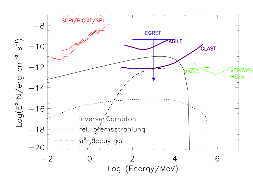
Fig. 2 shows the energy loss rates in comparison to the acceleration rate for a set of parameters typically found for colliding wind binaries. Obviously Coulomb losses dominate the low energy end of the electron spectrum, and simultanously provide a lower limit to the acceleration rate $a$. At energies $E\gtrsim m_{e}^{2}c^{4}/\epsilon_{T}$ Klein-Nishina effects significantly modify the energy loss rate due to inverse Compton scattering. Fig. 2 demonstrates that firstly, Klein-Nishina effects can in general not be neglected in the environment of colliding massive star winds. Secondly the curvature of the loss rate due to the Klein-Nishina decline of the inverse Compton cross section actually starts already at much lower electron energies. Consequently, in some cases the electron spectrum might be rather limited by synchrotron losses if the wind parameters are favourable. In the following, we take into account Klein-Nishina effects already above $E>E_{\rm TL}$ where $E_{\rm TL}$ is considered the energy below which the Klein-Nishina energy loss deviates not more than 20-25% from the Thomson limit approximation. Typically, for the systems considered in this work $E_{\rm TL}\approx 10^{-2}\mbox{MeV}/\epsilon_{\rm T,MeV}$ with $\epsilon_{T,MeV}$ the target photon energy in MeV.

In the extreme Klein-Nishina regime the total electron energy losses in the acceleration zone at high energies are effectively only provided by synchrotron radiation. In the transition range between the Thomson and Klein-Nishina limit, however, inverse Compton scattering may still dominate over synchrotron emission, thus mandating a proper treatment of the former. To allow for analytical solutions of Eq. 4 we approximate the Klein-Nishina decline of the loss rate in the transition range by

$$\dot{E}_{\rm IC,KN} = -b_{\rm IC,TL}E^{2}(1-E\epsilon_{\rm T,MeV}/5\cdot 10^{-2}\mbox{MeV})$$ (9)

for all energies $E<E_{s}=10^{-1.7\ldots-1.6}$MeV$/\epsilon_{\rm T,MeV}$, and

$$\dot{E}_{\rm IC,KN}\simeq-(0.27\sigma_{T}cn_{\rm ph,T}\epsilon_{\rm T,MeV}^{1/8}E+7\epsilon_{\rm T,eV}^{-1.846}*D_{14}^{-2}+2.1\cdot 10^{-4})\,\mbox{MeV/s}$$ (10)

$$=-(q_{a}E+q_{b})$$ (11)

for $E\geq E_{s}$ and with $n_{\rm ph,T}$ the integrated target photon density and $D_{14}$ the binary separation in $10^{14}$cm. These approximations are tested for $\epsilon_{\rm T}=1\ldots 100$eV, and are suitable for $0.01u_{\rm ph,T}\leq u_{\rm B}\leq u_{\rm ph,T}$ (while they deviate by more than an order of magnitude at energy $q_{a}/(2b_{\rm syn})\,[(1+\sqrt{(1-4b_{\rm syn}q_{b}/q_{a}^{2})}]$ if $u_{\rm B}$ decreases to $\leq 0.003u_{\rm ph,T}$).

This approximation is indicated in Fig. 2 by the long-dashed line and is suitable for cases where relativistic bremsstrahlung losses are much smaller than synchrotron or inverse Compton losses. While this approach takes reasonably into account the early deviation of the Klein-Nishina cross section from the Thomson cross section, it overestimates the energy loss rate in the extreme Klein-Nishina regime, which is mainly responsible for the steepness of the declining electron spectrum. Consequently, our derived electron and photon spectra shall be regarded with caution in their declining part.

The analytical solutions of Eq. 4 for electrons in the acceleration region are detailed in App. A. Fig. 3 shows examples of the resulting electron spectra for various values of the binary separation, while all other parameters are the same as used in Fig. 2. The general shape is determined by the interplay between acceleration gains and losses. At low energies Coulomb losses dominate and lead to the well-known upturn towards low energies due to the stronger increase of the acceleration rate with energy $\dot{E}_{\rm acc}\propto E$ when comparing to the competing radiative losses $\dot{E}_{\rm loss}\propto const$. For a reasonable convection velocity $V=1/2v_{\rm OB}$ (e.g. Luo et al., 1990) and assuming strong shocks $c_{r}=4$, a $\propto E^{-2}$ particle spectrum develops in the acceleration region if $\kappa_{a}/\kappa_{d}=4$, which we shall use in the following for demonstrative purposes if not noted otherwise. Thus in Fig. 3 a $E^{-2}$-spectrum develops until inverse Compton losses cause a steepening. The shape of this decline reflects the approximation employed to simulate the losses in the Klein-Nishina regime. The kink at $\sim 10^{3.5}$ MeV corresponds to the transition from the Thomson regime to the Klein-Nishina loss rate approximation. Finally, the cutoff at energy $E_{c}$ can be either due to radiative losses dominating over the acceleration rate, or the diffusion coefficient $\kappa_{d}$ approaching the Bohm limit $\kappa_{\rm Bohm}\approx 1/3r_{L}c$ where $r_{L}$ is the Larmor radius. In the latter case the escape time scale $T_{0}$ decreases with energy. For simplicity (and in order to keep the solutions analytical) we set $T_{0}=0$ at $\kappa_{d}\leq\kappa_{\rm Bohm}$ which then causes a sharp cutoff. More sophisticated calculations may smooth this decline towards an approximately exponential shape (Protheroe & Stanev, 2000). In the former case the cutoff is determined by the synchrotron loss rate that dominates regarding the flattening loss curve at high energies. In Fig. 3 the particle spectra cut off due to radiative losses for $D\leq 10^{14}$cm while at larger binary separations the Bohm limit causes the cutoff. Here both, synchrotron and inverse Compton losses, cease to be able to significantly affect the acceleration spectrum. For comparison we have also calculated electron spectra assuming isotropic diffusion. Fig. 4 shows the resulting spectra where all parameters are unchanged with respect to Fig. 3 except for the ratio of the diffusion coefficients $\kappa_{a}/\kappa_{d}$. As expected hard particle spectra with spectral index $s=1+p^{2}=1.25$ develop, and radiative losses alter the spectral shape depending on the binary separation. For $E\rightarrow E_{c}$ the spectra diverge for $((a-b_{\rm br})*T_{0})^{-1}<1$ (see Eq. A2, A4), which is fullfilled here.

Fig. 5 shows the energy loss rates in the convection zone for the same parameters as used for Fig. 2. On account of expansion in the cylindrical convection flow the magnetic field strength and the gas density fall off quickly with distance from the acceleration region. Coulomb interactions, bremsstrahlung, and synchrotron radiation will therefore loose importance as energy loss mechanisms and the inverse Compton scattering effectively provides the bulk of the electron energy losses.

Using a constant convection velocity the steady-state particle spectrum in the convection region can be found by solving Eq. 5. With the boundary conditions $N(E,r)\rightarrow 0$ for $r\rightarrow\infty$ and $N(E,r)\rightarrow N_{\rm acc}(E)$ for $r\rightarrow r_{0}$ where $N_{\rm acc}(E)$ is the steady-state particle spectrum in the acceleration region we derive the following analytical solutions using the standard method of characteristics: For $E<E_{\rm TL}$ the radiative losses are $\dot{E}=-b_{\rm syn\&IC}\,E^{2}$ and

$$N(E)=\left(\frac{r_{0}}{r}\right)^{2/3}\left[1+\frac{3b_{\rm syn\&IC}}{2V}Er\left(\left(\frac{r_{0}}{r}\right)^{2/3}-1\right)\right]^{-2}N_{\rm acc}(\tilde{E})$$ (12)

with

$$\tilde{E}=E\left(\frac{r}{r_{0}}\right)^{1/3}\left[1+\frac{3b_{\rm syn\&IC}}{2V}Er\left(\left(\frac{r_{0}}{r}\right)^{2/3}-1\right)\right]^{-1}$$ (13)

For $E\geq E_{\rm TL}$ an analytical solution can not be found using Eq. 9. In the convection region the approximation for the Inverse Compton energy losses in the Klein-Nishina regime, $E>E_{TL}$,

$$\dot{E}_{\rm IC,KN}=-q_{c}E$$ (14)

for $E_{\rm TL}<E<E_{\rm extr}$ with $q_{c}\approx b_{\rm IC}E_{\rm TL}$, and

$$\dot{E}_{\rm IC,KN}=-q_{d}$$ (15)

for $E\geq E_{\rm extr}=q_{d}/q_{c}$ with $q_{d}\approx 9/16c\sigma_{T}m_{e}^{2}c^{4}n_{\rm ph,T}\epsilon_{T}^{-1}$, turns out reasonable if $E_{\rm TL}$ is increased to $E_{\rm TL}\approx 10^{-1.7}\mbox{MeV}/\epsilon_{\rm T,MeV}$ (see Fig. 5). In this case the solution of Eq. 5 is

$$N(E)=\exp[\frac{q_{c}}{V}(r-r_{0})]\left(\frac{r_{0}}{r}\right)^{2/3}N_{\rm acc}(\tilde{E})$$ (16)

with

$$\tilde{E}=E\exp[\frac{q_{c}}{V}(r-r_{0})]\left(\frac{r}{r_{0}}\right)^{1/3}$$ (17)

for $E_{\rm TL}<E<E_{\rm ext}$, and

$$N(E)=\left(\frac{r_{0}}{r}\right)^{2/3}N_{\rm acc}(\tilde{E})$$ (18)

with

$$\tilde{E}=E\left(\frac{r}{r_{0}}\right)^{1/3}+\frac{3q_{d}}{4V}\left[\left(\frac{r}{r_{0}}\right)^{1/3}r-r_{0}\right]$$ (19)

for $E\geq E_{\rm ext}$.

The total solution is then combined such to assure continuity for all functions $E(r)$, $N(E,r,r_{0},N_{\rm acc}(\tilde{E}))$.

Fig. 6 shows the resulting electron spectrum in the convection region at $r=r_{0}\ldots 10^{14}$cm with a binary separation of $D=10^{14}$cm and using the parameters as described in Fig. 2 for the acceleration region. As the particles convect along $r$ radiative losses alter the high energy end of the particle spectrum leading to a decreasing cutoff energy with increasing $r$ while adiabatic losses lower the overall particle density. In Fig. 7 the binary separation has been enlarged to $D=10^{15}$cm. As a result radiative losses show a significant impact on the spectral shape only at large $r$.

In summary, taking into account convection in the extended emission region alters the energy cutoff in the integrated particle spectrum if radiative losses prove to be important, and simultanously lowers the total non-thermal particle density. This behaviour is reflected in the corresponding photon spectra (see Sect. 4).

3.2 Proton spectra

If protons are accelerated together with the electrons, hadronic nucleon-nucleon interaction take place with an approximated energy loss rate of

$$\dot{E}=-b_{\rm pp}E$$ (20)

above the kinematic threshold for pion production $E>E_{\rm thr}\simeq 0.28$ GeV (Mannheim & Schlickeiser, 1994),

$$b_{\rm pp}=1.3\times 3cN_{H}\sigma_{\rm pp}m_{\pi}/m_{p}\,$$ (21)

where $\sigma_{\rm pp}=3\cdot 10^{-26}$cm² is the corresponding hadronic cross section, and the factor 1.3 takes into account the here assumed metallicity (90% H, 10% He). Note that this linear relation for the energy loss rate is exact only above a nucleon kinetic energy of a few GeV, whereas at lower energies it shall be considered as an approximation. The corresponding error drops below $\sim 30\%$ above $\sim 10$ GeV. In addition, Coulomb-losses in the dense wind of the massive companion star of the WR-star will alter the injection spectrum. The Coulomb-losses are (Mannheim & Schlickeiser, 1994)

$$\dot{E}=-{{3\,c\,\sigma_{T}\,m_{e}c^{2}\,Z^{2}\,\ln\lambda}\over 2}\,N_{H}\,{{\beta^{2}}\over{x_{m}^{3}+\beta^{3}}}$$ (22)

with

$$\beta={\sqrt{E\,(E+2m_{p}c^{2})}\over{E+m_{p}c^{2}}}$$

and

$$x_{m}=0.2\,\sqrt{{T_{e}}\over{10^{8}\ {\rm K}}}\,.$$

The Coulomb-barrier occurs at $E_{m}\simeq 20\mbox{MeV}(T_{e}/10^{8}{\rm K})$ where $T_{e}\approx 10^{8}$ K is the electron temperature. We approximate the Coulomb-losses by

$$\dot{E}=-b_{\rm bel}E_{\rm MeV}$$ (23)

below the Coulomb-barrier with $b_{\rm bel}=6.6\cdot 10^{-16}Z^{2}N_{H}/x_{m}^{3}$ MeV/s, $E_{\rm MeV}$ is the particle kinetic energy in MeV, and

$$\dot{E}=\frac{-b_{\rm ab}}{\sqrt{E_{\rm MeV}}}$$ (24)

above the Coulomb-barrier with $b_{\rm ab}=6.7\cdot 10^{-12}Z^{2}N_{H}$ MeV/s. This approximation deviates at most a factor $\sim 2$ (by approaching the Coulomb-barrier) from the exact loss formula. In the relativistic regime, $\beta\geq 0.5$, we use

$$\dot{E}=-b_{\rm rel}$$ (25)

with $b_{\rm rel}=3.1\cdot 10^{-13}Z^{2}N_{H}$ MeV/s.

Eq. 4 describes the behaviour of the steady-state spectrum in the acceleration region. The solution, Eq. 7, can again be derived analytically (see App. B).

Fig. 8 shows examples of steady-state nucleon spectra with varying distance of the binary stars to each other. Close binaries show an upturn at low energies due to a high rate of Coulomb losses, and a spectral shape at larger energies that repeats the acceleration spectrum due to the same energy dependence of losses from hadronic $pp$-interactions and energy gain. For large binary separations Coulomb losses are unimportant, and the loss corrected particle spectrum has the same spectral shape as the steady-state acceleration spectrum. Due to the low hadronic cross section radiative losses hardly cause any cutoff in the particle spectrum. Instead, faster particle escape when approaching the Bohm diffusion limit leads to a steepening of the emitting particle distribution. For simplicity, we chose to treat this effect analog to the electron acceleration in Sect. 3.1, i.e. we set $T_{0}=0$ for $\kappa_{d}\leq\kappa_{\rm Bohm}$.

Applying mass conservation the continuity equation implies $N_{H}\propto r^{-1}$ for the target ion density $N_{H}$. With $r>r_{0}$, where $r_{0}$ indicates the transition from the acceleration to convection region with typically $r_{0}\sim 10^{12}$cm in the star systems considered here, hadronic $pp$-interactions and Coulomb-losses can readily be neglected. Eq. 5 can be solved to give the analytical solution for a constant convection velocity $V$:

$$N(E)=\left(\frac{r_{0}}{r}\right)^{2/3}N_{\rm acc}(\tilde{E})$$ (26)

with

$$\tilde{E}=E\left(\frac{r}{r_{0}}\right)^{1/3}$$ (27)

Fig. 9 shows the resulting nucleon spectrum for the same parameter set as used in Fig. 6. Obviously the losses due to $pp$-interactions are of minor importance as compared to the adiabatic losses the nucleons suffer in the convection region.

3.3 Particle spectra normalization

For applications to massive binary systems the normalization of the relativistic particle component is limited by several constraints: Firstly, the inverse Compton, bremsstrahlung and $\pi^{0}$-decay $\gamma$-rays must not overproduce any observational limits imposed by $\gamma$-ray observations (e.g. EGRET, …). Secondly, since the particles are accelerated out of the pool of thermal particles, particle number conservation dictates that the relativistic particle flux injected into the system must be smaller than the wind particle flux entering the acceleration zone, i.e. $Q_{0}\leq\dot{M}/(m_{p}\,x^{2}4\pi\,d)$ with $d$ the thickness of the acceleration site. Furthermore, due to energy conservation the total injected particle energy can not be larger than the total kinetic wind energy of the binary system which rarely exceeds 1% of the total radiative energy output of the stars, (typically $L_{\rm w}\leq 10^{37}$erg/s). The energy density of accelerated particles is given by $U_{\rm acc}\approx Q_{0}E_{0}/a$ assuming an $E^{-2}$-spectrum ($aT_{0}=1$). In equilibirium the total acceleration power equals the loss power due to escape, leading to $L_{\rm acc}=U_{\rm acc}V_{\rm acc}/T_{0}$ where $V_{\rm acc}=r_{0}^{2}\pi d$ is the acceleration volume. By noting that $(r_{0}^{2}/4x^{2})L_{\rm w}$ is the kinetic power available to the acceleration region, $Q_{0}$ can not exceed $Q_{0}\sim(r_{0}^{2}/4x^{2})L_{\rm w}/(V_{\rm acc}E_{0})=L_{\rm w}/(4x^{2}\pi dE_{0})$. These latter two arguments pose to date a stronger constraint on the normalization than the $\gamma$-ray limits from EGRET. In the following we use this maximum possible injection power unless stated otherwise.

4 Photon spectra

This work is devoted to photon emission at high energies with emphasis on the $\geq 1$ MeV regime. Important non-thermal continuum emission processes here are inverse Compton scattering of the dense stellar radiation field to high energies, relativistic bremsstrahlung of the electrons in the field of the ions in the wind and the decay of $\pi^{0}\longrightarrow\gamma+\gamma$ that are produced in hadronic nucleon-nucleon collisions. For the calculations of the photon spectra we assume the particle distributions to be isotropic in the wind-wind collision zone.

4.1 Inverse Compton scattering

Inverse Compton (IC) scattering in the dense UV stellar radiation field of the massive main sequence star often dominates photon production rate at high energies. The computation of the photon emission is based on the full Klein-Nishina cross section while for the IC losses of the electrons either the cross section in the Thomson limit or the Klein-Nishina approximations Eq. (9, 11, 14) are applied assuming the losses to be continuous. We have further neglected triplet pair production, since the value of $\epsilon_{T}E/m_{e}c^{2}$ that we consider does not exceed $10^{3}$ (Mastichiadis, 1991). We restrict this work to long-period binary systems, for which the wind momentum from the WR-star clearly dominates, thus placing the WR-star at a large distance from the collision region. This allows us to neglect the stellar radiation field of the WR-star as a target photon field for IC scattering. For the stellar radiation field of the OB-star the monochromatic approximation

$$n(\epsilon,\mu_{\rm ph})=n_{0}\,\delta(\epsilon-\epsilon_{T})\,\delta(\mu-\mu_{\rm ph})$$ (28)

with $\epsilon_{T}=2.7\,k_{B}T_{\rm eff}$ is employed. All seed photons are approaching the emission region from the same direction. In this case the full angular dependence of the IC scattering rate has to be taken into account, since the scattered power per volume element depends on the scattering angle $\theta_{\rm ph}$. In appendix C we calculate the IC photon production rate, $\dot{n}(\epsilon_{s},\Omega_{s})$, for an arbitrary target photon field $n(\epsilon,\mu_{\rm ph})$ that scatters off an isotropic electron distribution. We find a declining scattering rate with decreasing scattering angle $\theta_{\rm ph}$, in agreement with earlier works (Reynolds 1982a, ; Brunetti, 2000, ; see Fig. C.1). The volume-integrated emitted photon power is calculated by

$$\dot{N}_{\rm IC}(\epsilon_{s})=\int dV\ \dot{n}(\epsilon_{s},\Omega_{s})=d\times\int drr\int d\phi\dot{n}(\epsilon_{s},\Omega_{s})$$ (29)

where the integrals have been solved numerically. The IC flux variations directly translate into a change of IC power and maximum energy with viewing angle $\theta_{\rm ph}$ (see Fig. 10). For a given system inclination the total emitted power and maximal scattered energy therefore varies with orbital phase (Fig. 11). These anisotropy effects may be detectable with near future $\gamma$-ray experiments like GLAST (see Sect. 6). For a non-negligible size of the convection zone the volume integration may lead to photon spectra that show a kink. This feature occurs at energies above which the convection zone is lacking high energy particles. The combined effect of both, a deficit of high energy particles in the convection zone and a visible increase of the total flux from the convection zone, results in the kink at 1-10 MeV in Figs. 10,11.

4.2 Relativistic bremsstrahlung

Non-thermal relativistic bremsstrahlung losses are non-negligible in the stagnation point of the colliding winds where the (compressed) gas density may reach values of $10^{5\ldots 9}$cm^-3 whereas in the convection region the decreasing gas density makes its contribution minor. The nonthermal bremsstrahlung photon flux using a typical ISM metallicity (90% H, 10% He, neglecting contributions from higher atomic number particles)

$$\dot{N}_{\rm ph,br}(E_{\gamma})=\frac{1.3N_{H}c}{4\pi d_{L}^{2}}\int dV\int_{\max(E_{\gamma}m_{e}c,E_{\rm min})}^{E_{\rm max}}dE\ N(E)\,\frac{d\sigma}{dE_{\gamma}}$$ (30)

is calculated numerically in the relativistic limit (valid for $E/m_{e}c^{2}\geq 15/Z$, $Z$ is the atomic number) using the differential cross section from Blumenthal & Gould (1970). Examples of bremsstrahlung spectra are shown in Fig. 12 for the electron spectra in Fig. 3. The shape of the bremsstrahlung photon spectrum in the relativistic regime reflects the shape of the electron spectrum. The larger the binary separation is, the larger is the difference between the turnover energy from the Thomson to KN-loss regime and the cutoff energy (see Fig. 3). This leads to a decline of the bremsstrahlung spectrum at an energy that increases with the binary separation. An estimate of the thickness $d$ of the emission region was provided by Eichler & Usov (1993) who showed that $d\approx x=x_{\rm OB}$. With $r_{0}\approx 10^{12}$cm the total emitting volume in the acceleration region is $\pi r_{0}^{2}d\approx 10^{38\ldots 39}$cm³. Fig. 12 shows the resulting relativistic bremsstrahlung power spectra for various binary separations. Despite a somewhat larger emitting volume for colliding wind systems with a large binary separation, the total bremsstrahlung emission declines with binary separation due to a rapidly decreasing target gas density in the collision region. For $D=10^{14}$cm the compound acceleration and convection region spectrum is also presented in Fig. 12. Due to the volume effect the dominant contribution to the total emission spectrum comes from the convection region at large $r$, thus increasing the overall bremsstrahlung intensity. At the same time the deficit of high energy particles in the convection region at large distances from the acceleration region (see Fig. 6) leads to a deficit of high energy photons. This causes the feature at $\sim 100$ MeV in the total bremsstrahlung spectrum shown in Fig. 12 (plotted for a $D=10^{14}$cm binary separation).

4.3 $\pi^{0}$-decay $\gamma$-ray emission

Collisions between cosmic ray protons and nucleons in massive star winds are rather rare and occur on average a few times per year for gas densities in the wind collision region typical for long-period binaries like WR 140.

The stationary proton spectra as shown in Fig. (8, 9) are used to calculate the $\pi^{0}$-decay photon spectrum. Since the proton spectra above the threshold for $pp$-interactions in general reflects the shape of the acceleration spectrum, one expects pure power law particle spectra in this energy range. The formalism developed by Pfrommer & Enßlin (2004) for the $\pi^{0}$-decay $\gamma$-ray production of pure power law particle spectra seems therefore appropriate to use. The resulting $\pi^{0}$-decay $\gamma$-ray spectra (calculated for a ⁴He mass fraction of 0.3 for the wind metallicity; see Sect. 4.2) from the acceleration region are shown in Fig. 13 for various binary separations. The uppermost curve corresponds to the combined acceleration and convection region $\pi^{0}$-decay spectrum for a binary separation of $D=10^{14}$ cm.

For typical parameters of colliding massive wind systems and maximal allowed injection power the radiative luminosity from $\pi^{0}$-decay lies therefore typically on a $\leq 10^{33}$erg/s flux level, leading to a $\pi^{0}$-decay luminosity from wide binary systems that can in general be neglected when compared to the expected IC-luminosity $>$1 GeV, provided the emitting electron spectrum extends to $\geq 10^{4}$ MeV.

4.4 $\gamma-\gamma$ opacity in the stellar radiation fields

Above $\sim 100$ GeV the optical depth $\tau_{\gamma\gamma}$ due to photon-photon pair production ($\gamma\gamma\rightarrow e^{+}e^{-}$) in the intense stellar radiation field of the main sequence star may reach non-negligible values depending on its spectral type. This may modify the $\gamma$-ray spectrum escaping from the source by a factor $\exp(-{\tau_{\gamma\gamma}})$.

The $\gamma-\gamma$ opacity $d\tau_{\gamma\gamma}$ along a path element $dy$ in a radiation field with differential photon number density $n(\epsilon,\Omega)$ is given by (Gould & Schreder, 1967)

$$d\tau_{\gamma\gamma}(E_{\gamma},\epsilon,\Omega)=dy\,n(\epsilon,\Omega)\,\sigma_{\gamma\gamma}(\epsilon,E_{\gamma},\mu_{\gamma\gamma})\,(1-\mu_{\gamma\gamma}).$$ (31)

With the target photon density

$$n(\epsilon)=n_{0}\,{{r_{s}^{2}}\over{\tilde{x}+y^{2}+2y\mu_{\rm ph}\sqrt{\tilde{x}}}}\,\delta(\epsilon-\epsilon_{T})\,\delta(\mu-\mu_{\gamma\gamma})$$

above the stellar radius $r_{s}$, and $\tilde{x}=x^{2}+r^{2}$, this can be re-written as

$$\tau_{\gamma\gamma}(E_{\gamma},\mu_{\rm ph},x,r)=\frac{n_{0}(\epsilon=\epsilon_{T})r_{s}^{2}}{8\pi E_{\gamma}\epsilon_{T}}\int d\phi\int_{0}^{\infty}dy\frac{s\sigma_{\gamma\gamma}(s)}{\tilde{x}+y^{2}+2\,\sqrt{\tilde{x}}\,y\,\mu_{\rm ph}(\theta_{L},\phi_{L},\cos{\theta}=x/\sqrt{\tilde{x}},\phi)}\,H(s-s_{\rm thr})$$ (32)

for photons of energy $E_{\gamma}$ escaping from the emission region at location $r$ along a path $y$ with angle $\theta_{\rm ph}=\cos{\theta_{L}}\,\cos{\theta}+\sin{\theta_{L}}\,\sin{\theta}\,\cos(\phi-\phi_{L})$. Here, $s=2\,E_{\gamma}\,\epsilon(1-\mu_{\gamma\gamma}(y))$ is the square of the centre of momentum (CM) energy, $\sigma_{\gamma\gamma}(s)$ the cross section for photon-photon pair production (Gould & Schreder, 1967), $s_{\rm thr}=(2m_{e}c^{2})^{2}$ is the squared minimum CM energy required to overcome the process threshold, $\mu_{\gamma\gamma}(y)=\cos{\theta_{\gamma\gamma}(y)}$ is the cosine of the angle between the two interacting photons. and $\cos{\theta}=x/\sqrt{x^{2}+r^{2}}$.

In Fig. (14-16) we show the absorption optical depth due to photon-photon collisions in a $T=43000$ K radiation field (i.e. $\epsilon_{T}=10$ eV) for different $r_{\rm OB}=1.2-24\cdot 10^{13}$cm being the separation of the emission region from the stellar photosphere, and for various angles $\theta_{L}=0\arcdeg-180\arcdeg$, respectively. Large viewing angles decrease the process’ threshold energy in the observer frame, and increase the opacity at the same time due to a longer path way and the rise of the CM energy. Fig. 14 shows that variations of the optical depth with angle $\theta_{L}$ by several orders of magnitude are possible, and absorption can be quite severe (up to $\tau_{\gamma\gamma}\sim 100$ for $D=10^{14}$cm). Except at large $\theta_{L}$ the effect of varying $r$ mainly impacts the absorption depth near threshold (see Fig. 15). The opacity is also strongly dependent on the radiation field density which is dependent on the massive star’s luminosity as well as on $r_{\rm OB}$. This can be observed in Fig. 16 where $\tau_{\gamma\gamma}$ ranges between 0.002 to 0.04 at the peak of the cross section and along the $\theta_{L}=45\arcdeg$ sight line.

This essay shows that $\gamma$-ray absorption due to pair production can not be neglected in general for massive star systems, but must be treated individually for each system and is strongly dependent on the sight line.

5 Applications

5.1 WR 140

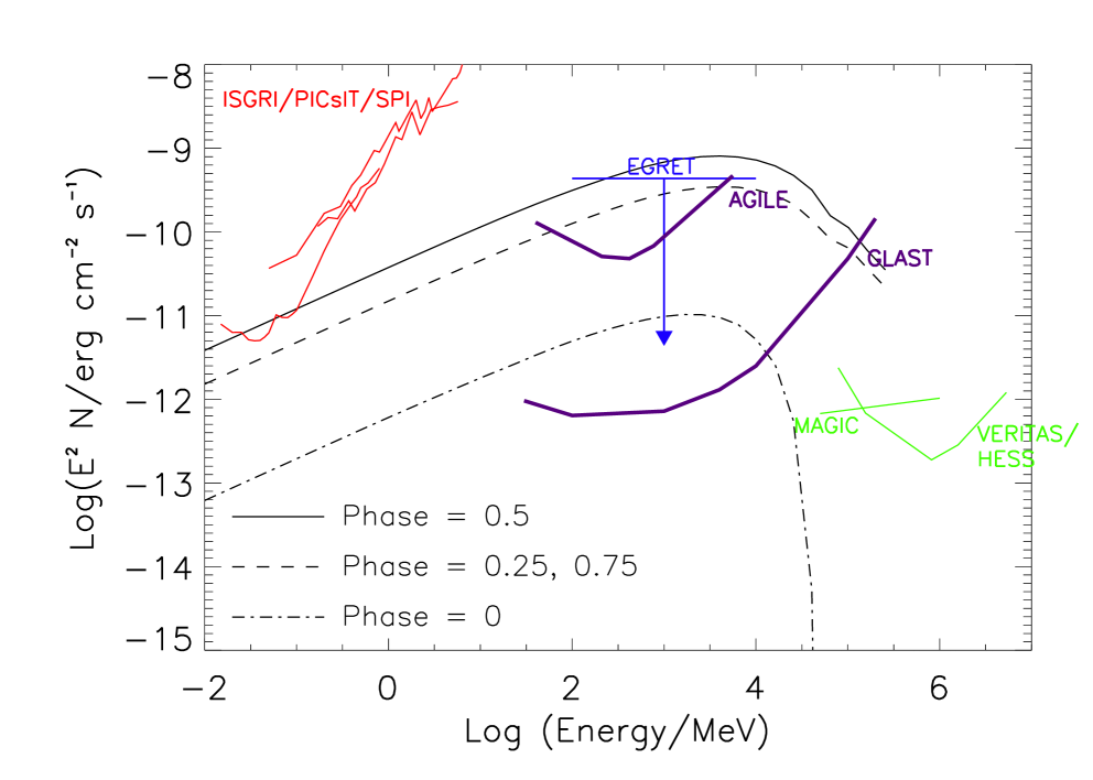
WR 140 (catalog ) is the archetype of a spectroscopic long-period massive binary system of colliding winds which shows periodic dust formation around periastron passage as well as nonthermal radio emission at phases where the colliding wind region is outside the photosphere for free-free absorption. The system has been well monitored at radio, IR, optical, UV and X-rays (e.g. Williams et al., 1990; White & Becker, 1995; Panov et al., 2000; Setia Gunawan et al. 2001b, ). It consists of a WC 7pd and a O4-5 V companian (of bolometric luminosity $L_{\rm bol}=10^{5.8}L_{\sun}$ and effective temperature $T_{\rm eff}=43000$ K) with an orbital period of $2899\pm 10$ days. Located at a distance of 1.85 kpc (Dougherty et al., 2005) the large inclination system ($i=122{\arcdeg}\pm 5{\arcdeg}$; Dougherty et al., 2005) possesses an excentricity of $0.881\pm 0.04$. With periastron passage being defined by phase $\Phi=0$ the argument of periastron is $\omega=47\arcdeg$ (Marchenko et al., 2003). In this work we use the basic parameters that has been recently re-determined by Dougherty et al. (2005). The mass loss rate of $8.7\cdot 10^{-6}M_{\sun}$/yr and the wind velocity of the O-star $v_{\rm OB}=3100$ km/s as compared to the mass loss rate of $4.3\cdot 10^{-5}M_{\sun}$/yr of the WR-star at velocity $v_{\rm WR}=2860$ km/s places the collision region at a distance of $x\approx 0.32D\approx 9.6\cdot 10^{12}\ldots 1.5\cdot 10^{14}$cm from the O-star due to momentum balance and taking also into account the excentricity of the system. This is a factor $\sim 2.5$ smaller than used in earlier works (e.g. Eichler & Usov, 1993; Benaglia & Romero, 2003). At this distance the wind gas density lies between $\sim 4\cdot 10^{6}\ldots 9\cdot 10^{8}$cm^-3. For the strength of the shock we assume a compression factor $c_{r}=4$. The radio emission reaches its maximum roughly at phase 0.83. The nonthermal radio spectrum at phases $\Phi=0.671\ldots 0.955$ shows typically a $\alpha=-0.5$ spectrum, indicating that the underlying particle distribution obeys a power law with spectral index $p=2$ (Williams et al., 1990; Dougherty et al., 2005). The spectral requirements are in agreement with a convection velocity of $\sim 1410\ldots 1540$ km/s in the framework of our simplified geometrical picture. For predicting WR 140’s high energy emission from primary electrons and protons we have selected four orbital phases approximately equally separated where its non-thermal radio emission has been determined (Dougherty et al., 2005), namely $\Phi=0.995$, 0.2, 0.671 and 0.8. In order to reproduce the flux level of the cm radio data for those phases we require a energy injection rate of thermal particles that varies with orbital phase and lies between $10^{32.5\ldots 33.5}$ erg/s or $10^{-3}\ldots 10^{-2}\%$ of the OB-wind kinetic energy. The total emission volume $V=r^{2}_{\rm max}\pi d$ with $d\sim x$ is also assumed to vary with orbital phase (we used $r_{\rm max}=4\cdot 10^{14}$cm for $\Phi=0.2$, 0.671 and 0.8, and $r_{\rm max}=10^{13}$cm for $\Phi=0.995$) as suggested by the cm radio observations (Dougherty et al., 2005). The magnetic field at the O-star surface is assumed of order 100 G, which leads to field values of 0.2 …3.5 G in the wind collision zone (in agreement with estimates for the equipartition magnetic field: Benaglia & Romero, 2003). The diffusion coefficient $\kappa_{\rm a}$ determines the acceleration rate and, together with the energy loss channels, the maximum particle energy. In order to allow for relativistic electron energies, necessary to explain the observed synchrotron radiation, $\kappa_{\rm a}$ must be low enough that acceleration gains are able to overcome the Coulomb losses. On the other side, Bohm diffusion is the limit for the diffusion coefficient $\kappa_{\rm d}$, which is connected to $\kappa_{\rm a}$. This leads to a rather narrow range of possible values for the diffusion coefficients if one requires the production of $>100$ MeV photons via the IC process at least at phases close to apastron. For our models presented in Fig. 18, 19, 20 we used $\kappa_{\rm a}=3.76\cdot 10^{19}$ cm²/s which results in an acceleration region size of $r_{0}=2.4\ldots 2.6\cdot 10^{11}$ cm and escape time of $T_{0}=1.6\ldots 1.9$ks. Detections of the maximum photon energy will shed light on the exact value of $\kappa_{a}$.

Fig. 17 shows the steady-state electron spectra at orbital phases 0.955 (close to periastron), 0.2, 0.671 (close to apastron) and 0.8 for these parameter values. Due to the excentricity of the system the wind collision region is located closest to the main sequence star at periastron while it is furthest away at apastron. All spectra except at periastron extend to very high energies with the cutoff due to the finite size of the acceleration region, and a smooth change in the spectral index where Klein-Nishina effects set in. The sharpness of the cutoff is a result of the approximations employed in this work, and may appear somewhat softened in more sophisticated (however then indispensably non-analytical) calculations.

At periastron the wind collision region is closest to the OB-star, and the electron spectrum is cutoff already at $\sim$100 MeV due to (Thomson regime) IC losses in the intense photospheric radiation field. Fig. 19 and 20 shows the corresponding broad band SEDs in comparison with the sensitivity of the INTEGRAL instruments, GLAST, AGILE and the current generation IACTs like H.E.S.S., MAGIC and VERITAS. The EGRET upper limit has been derived from the summed P1-P4 EGRET data at the location of WR 140 (see also Mücke & Pohl, 2002). At all orbital phases IC emission dominates over all other radiation processes except close to periastron. Here the IC spectrum cuts off already at a few MeV, corresponding to the cutoff in the electron spectrum. The $\gamma$-ray domain is therefore only covered by relativistic bremsstrahlung radiation (up to $\sim$100 MeV following the electron spectrum) and $\gamma$-rays from the $\pi^{0}$-decay. (Ion-electron) bremsstrahlung emission turns out to lie always below the IC photon output at a level that is not detectable for current and near future instruments. Assuming the maximal possible injection rate of thermal particles into the acceleration region, $\pi^{0}$-decay $\gamma$-rays may possibly be detected with GLAST at orbital phases close to periastron where the density of the target material is enhanced. At apastron the losses in the photospheric radiation field as well as due to the wind particle density are low enough to allow the photon spectra to extend into the 10-100 GeV regime with a IC flux level detectable, particularly with low-energy threshold IACTs (e.g. MAGIC) and GLAST. This is true despite photon absorption from pair production which leaves its fingerprint above $\sim$100 GeV (see Fig. 20: at $\Phi=0.67$ $\tau_{\gamma\gamma}(r=r_{0},E\approx 100\mbox{GeV})\sim 1$ while at $\Phi=0.95$ $\tau_{\gamma\gamma}(r=r_{0},E\approx 100\mbox{GeV})\sim 3$).

Fig. 18 zooms onto the IC spectra. The flux variations due to the anisotropy effect at different orbital phases are blurred by flux variations due to the changes in the radiation field density in the strongly excentric system. The feature at $\leq 1$ MeV stems from the deficit of high energy particles in the convection zone. For this parameter setting we predict a maximum of the IC flux at phase $\Phi\simeq 0.95$, the minimum IC flux level would occur at phase $\sim 0.01$. Thus the next maximum $\gamma$-ray flux level is expected around August 2008, just in time for a clear detection with GLAST.

5.2 WR 147

WR 147 (catalog ), a WN8(h) plus B0.5 V (with bolometric luminosity of $L_{\rm bol}=5\cdot 10^{4}L_{\sun}$ and effective temperature $T_{\rm eff}=28500$ K, i.e. $\epsilon_{T}\approx 6.6$ eV) massive binary system is among the closest and brightest systems that show non-thermal radio emission in the cm band. Owing to its proximity this system has been resolved in a northern non-thermal component (WR 147N) and a southern thermal one (WR 147S) with a separation of $575\pm 15$ mas using the MERLIN instrument (Churchwell et al., 1992; Williams et al., 1997). The observed radio morphology and spectrum supports a colliding wind scenario for WR 147 (catalog ), as first proposed by Williams et al. (1997). At a distance of 650 pc the implied binary separation is estimated to 417 AU. The mass loss rates ($\dot{M}_{\rm WR}=2.5\cdot 10^{-5}M_{\sun}$/yr, $\dot{M}_{\rm OB}=4\cdot 10^{-7}M_{\sun}$/yr) and wind velocities ($v_{\rm WR}=950$ km/s, $v_{\rm OB}=800$ km/s) place the stagnation point at $6.6\cdot 10^{14}$cm, in agreement with the MERLIN observations. A comprehensive study of the WR 147’s radio emission and the geometry of the system has been presented by Setia Gunawan et al. 2001a . Any excentricity nor the inclination of the system are known so far, hence we assume $i=90{\arcdeg}$ and $e=0$ for this application to WR 147. The non-thermal flux component can be well fitted by a power law with spectral index $\alpha=-0.43$ with, however, poor statistical significance. For our presentation we use again the canonical value of $\alpha=-0.5$ corresponding to an $E^{-2}$ power law particle spectrum. Assuming strong shocks, a convection velocity of 399 km/s and a B-star surface magnetic field of 30 G (translating into a 25 mG field strength in the wind collision region, close to its equipartition value (Benaglia & Romero, 2003)) the observed radio flux level can be reproduced if $\sim 0.15\%$ of the OB-wind kinetic energy is injected as thermal particles into the emission region of a total estimated volume of $\sim 2.6\cdot 10^{5}$AU³. Again the diffusion coefficient is chosen such to overcome Coulomb losses and allow the production of $>100$ MeV through the inverse Compton process without violating the Bohm-limit at the same time. With $\kappa_{\rm a}=2\cdot 10^{21}$ cm²/s convection is dominant in $\sim 90\%$ of the total emission region, and the acceleration site covers a size of $r_{0}=5\cdot 10^{13}$ cm (escape time is $T_{0}\approx 10^{6}$s).

In Fig. 21 the resulting steady-state electron spectrum is shown. For a negligible system eccentricity it is the same at all orbital phases. The steepening at $10^{4\ldots 5}$MeV is due to synchrotron losses, the slight upturn towards lower energies reflects the influence of the Coulomb-losses. Above $\sim 10^{5.5}$MeV the Bohm-limit cuts off the particle spectrum. Fig. 22 demonstrates the orbital IC flux variations due to the anisotropic nature of the IC scattering of more than one order of magnitude for the chosen system inclination. The maximum flux level is expected when the WR-star is behind the OB-star along the sight line. These flux changes will be in principle detectable for GLAST at all orbital phases, and also for low-threshold IACTs provided high particle energies are reached, which by itself depends on the acceleration rate. Thus measurements with IACTs will be able to place important constraints on the acceleration efficiency in these environments. The EGRET upper limit is taken from Benaglia & Romero (2003). For an estimated wind gas density of up to $1.4\cdot 10^{5}$cm^-3 non-thermal bremsstrahlung emission stays several orders of magnitude below the IC flux level, not detectable with current instruments to date. Also the contribution from $\pi^{0}$-decay $\gamma$-rays remains negligible, even for a maximal possible thermal particle injection rate. For WR 147, being a extremely long-period binary with an assumed small excentricity, the photospheric UV radiation field at the location of the collision region is low enough to allow here the neglection of $\gamma$-ray absorption due to photon-photon collisions.

6 Detectability from soft to very high energy gamma-rays

6.1 Soft gamma-ray instruments

The regime of soft gamma-rays, here considered to be typical ranging from 511 keV up to several MeV, is currently only accessible by the IBIS and SPI instruments aboard INTEGRAL. Previous mission like SIGMA/GRANAT and COMPTEL did not reported the detection of soft gamma-ray emission from the WR systems studied here. Given the continuum sensitivity of the IBIS and SPI instruments, accordingly scaled for a common observation time of $10^{6}$ sec in order to achieve a 3 $\sigma$ detection, the detection of WR 140 appears to be possible at soft gamma-rays only if significantly more observation time than 1 Msec will be dedicated to observations towards such an object. Hard X-ray emission may be seen by ISGRI, most favorably in orbital phases where the line of sight towards an observer is parallel to the contact discontinuity of the wind collision zone or when both the WR and O star are nearly aligned and the wind collision zone is most pronouncedly exposed towards the observer. At soft gamma-rays, even in the most favorable orbital states, several Msec may be required to pick up emission from WR 140 (Fig. 18). This situation is very similar for WR147 (Fig. 22).

6.2 High-energy gamma-ray instruments

At energies between 30 MeV and 10 GeV, detection claims of gamma-ray emission from WR binary systems have been made already from COS-B observations. More particular, WR 140 (HD193793) was considered to be associated with the variable COS-B source 083+03 (Pollock, 1987), a source exhibiting a photon flux at the $5\cdot$10^-7ph cm^-2s^-1 level at E $>$ 300 MeV. However, this individual association could not be confirmed by observations of the EGRET instrument aboard CGRO, which would have seen a source at the $\sim 1.5\cdot$10^-6ph cm^-2s^-1 at E $>$ 100 MeV. Although a number of positional coincidences between unidentified EGRET sources and colliding wind binary systems has been noted by (Kaul & Mitra, 1997) and (Romero et al., 1999), the individual case for an association between WR 140 and the unidentified EGRET source 3EG J2022+4317 appears to be vague on the basis of the given observational evidence at $\gamma$-rays. 3EG J2022+4317 is cataloged (Hartman et al., 1999) with a flux of $2.5\cdot$10^-7ph cm^-2s^-1, and the spectrum fitted with a power-law with an index of 2.3 $\pm$ 0.2; it is further to be characterized by a rather irregular uncertainty contour pointing towards source extension, and indication of source confusion above E $>$ 100 MeV. The EGRET observations were taken within the first four years of the CGRO mission between 1991 and 1994, with the gross obtained toward the periastron phase of the binary system. In the sparse EGRET observations above the detection threshold of the 3EG catalog there is no evidence for variable $\gamma$-ray emission (Nolan et al., 2003). Since WR 140 is at a distance of 0.67^o to the nominal position of 3EG J2022+4317, and only barely consistent with the 99$\%$ source location uncertainty contour, which prevents any conclusive identification between both objects, it is appropriate to determine an upper limit at the position of WR 140 under consideration that $\gamma$-ray emission of 3EG J2022+4317 is fully taken into account but not been associated with WR 140 (Mücke & Pohl, 2002). This upper limit is consistent with our predictions given in Fig. 18, considering that EGRET observations were performed over a superposition of orbital states including the periastron phase, where the cutoff due to IC losses in the Thomson regime will not allow any detectable $\gamma$-ray emission at all at energies above a few MeV. Since AGILE will exhibit a similar sensitivity characteristics compared to the EGRET instrument, chances for AGILE to clarify on 3EG J2022+4317 are only given if AGILE is operated in orbit over a long period. The instrumental sensitivity of AGILE is indicated for a 5 $\sigma$ detection on the basis of $10^{6}$ sec observation time. Thus, it’ll be the Gamma-ray Large Area Space Telescope (GLAST) to give an observational reassessment of the unidentified EGRET source 3EG J2022+4317 and its association or non-association with WR 140. Clearly, GLAST exhibits a sensitivity characteristics to achieve a detection not only from observations accumulated over various orbital states of the colliding wind binary, it has a dedicated chance to provide results from individually selected orbital states. As mentioned above, during periastron phase there is no high-energy $\gamma$-ray emission predicted (Fig. 19), but the changes in the $\gamma$-ray flux of WR 140 when going into periastron or coming out of periastron phase will be detectable, since the sensitivity of GLAST will be indeed sufficient to detect this system in the more favorable orbital states when the edges of the contact discontinuity of the wind collision zone lines up in the line-of-sight or the wind collision zone is most extensively exposed towards the observer. GLAST will have this detection potential up to energies where the the finite acceleration site cuts off the emission, approximately up to $\sim$ 50 GeV. The chance to detect high-energy emission in case of WR 147 with future instruments is even somewhat better than for WR 140. If AGILE with its better instrumental point spread function than EGRET will be able to distinguish the location of WR 147 from the bright $\gamma$-ray source 3EG J2033+4118, its sensitivity will be sufficient to observe $\gamma$-ray emission over the majority of favorable orbital states (Fig. 22). However, the periastron phase will still be out of reach for AGILE, see Fig. 23. GLAST, again, will have the instrumental capability to both distinguish a test position at the location of WR 147 ($l=79.85,b=-0.32$) from the presumably bright $\gamma$-ray source 3EG J2033+4118. Depending on a possible contribution of further sub-threshold sources in the vicinity of 3EG J20233+4118, this might not be too straight forward, though.

6.3 VHE gamma-ray instruments

Complementary to the satellite experiments operated at soft and high-energy $\gamma$-rays, the continuous development of the Imaging Atmospheric Cherenkov Telescopes (IACTs) towards better sensitivity, even more improved angular resolution, and lower energetic thresholds, clearly exhibit the capability to detect $\gamma$-ray emission produced in colliding winds of massive stars in binary systems. Especially the chance to accumulate a wealth of photons on sub-hour time scales will enable the IACTs to test the predicted orbital flux variations precisely. A unique chance to detect emission from WR 140 is given for those experiments able to work at the lowest possible threshold, i.e. MAGIC below 100 GeV. Depending on the actual shape of the cutoff due to the finite site of the acceleration site, events may be seen only in extreme low-energetic event selections, and the respective sky location is further characterized by an absence of higher energetic photons. For an array of IACTs like VERITAS (Weekes et al., 2002) the best sensitivity is achieved at energies above the cutoff due to the finite acceleration site in WR 140, subsequently making any detection prospects heavily dependent on the actual shape of the cutoff. IACT arrays located in the southern hemisphere like H.E.S.S., or CANGAROO may not have the chance detect this system at all due to the higher energetic threshold when observing under low zenith angle conditions. In case of WR 147, where the orbital parameters are more promising to detect high-energy $\gamma$-ray emission up to several hundreds of GeVs, low threshold IACTs located in the northern hemisphere will have a distinct chance to detect WR147 in non-periastron orbital phases (Fig. 22), provided that the $\gamma$-ray analysis will not introduce hard cuts for preference of a higher energetic event selection. For both satellite and ground-based instruments the colliding wind zone will not appear to be spatially resolved, presenting individual colliding wind binary systems as point-source candidates at the $\gamma$-ray sky.

7 Conclusions and discussion

In this work we have calculated the emission from non-thermal steady-state particle spectra built up in the regions of colliding hypersonic winds (assumed to be homogeneous) of long-period massive binary systems with the stagnation point defined by balancing the wind momenta and under the assumption of spherical winds. The shocked high-speed winds are creating a region of hot gas that is separated by a contact discontinuity. The gas flow in this region away from the stagnation point will be some fraction of the wind velocity which we kept constant here. A simplification of the geometry from a bow-shaped to a cylinder-shaped collision region allowed us to solve the relevant diffusion-loss equations analytically. We considered first order Fermi acceleration out of a pool of thermal particles, and took into account radiative losses (synchrotron, inverse Compton including Klein-Nishina effects, bremsstrahlung and Coulomb losses), (energy-independent) diffusion by introducing a constant escape time $T_{0}$ and convection/advection with constant speed. Above a certain distance from the stagnation point convection dominates over diffusion with the transition point determined by balancing the diffusion and convection loss time. Correspondingly, we devided the emission region into a region where acceleration/diffusion dominates, the ”acceleration zone”, and the outer region where convection/advection dominates, the ”convection zone”.

Electrons may reach relativistic energies, once they overcome the heavy Coulomb losses in the dense shocked material, through diffusive shock acceleration up to the Bohm diffusion limit. For wide binary systems this latter constraint is often severe, while for close binaries, radiative losses mostly cause the cutoff. Taking into account existing upper limits of the stellar surface magnetic field strength of massive stars, inverse Compton losses in general dominate over synchrotron losses if in the Thomson loss regime. We have shown, however, that losses may well extend into the transition region leading to the extreme Klein-Nishina regime. The flattening of the Compton loss rate there may in some cases cause the synchrotron losses dominate eventually. Thus a rigorous treatment of the Compton losses must include Klein-Nishina effects. For this purpose we have derived analytical approximations for Klein-Nishina losses that are suitable for massive binary systems, and allow at the same time to solve the relevant diffusion-loss equation analytically. Despite the high density environment of the emitting collision region, non-thermal bremsstrahlung losses prove general to be of minor importance. This turns out to be true also for the corresponding radiation.

We have studied inverse Compton radiation, the main emission channel for relativistic electrons in these systems, in severe detail. The use of the full Klein-Nishina cross section leads to a spectral softening at the high-energy end of the emitted radiation. Since the stellar target photons for inverse Compton scattering arrive at the collision region from a prefered direction, the full angular dependence of the scattering process has to be considered. Its anisotropic nature leads to variations of the flux level by up to several orders of magnitude (depending on system inclination and eccentricity) as well as cutoff energy with orbital phase. The maximum flux and cutoff energy occurs when the WR-star lies behind the OB-star. We consider therefore massive binary systems as $\gamma$-ray sources that are variable on the time scale of their orbital period even in the absence of a strong system eccentricity. The inclusion of convection/advection effects into the calculation of the particle spectra reveals a possibly visible spectral feature, too. Because of a deficit of low-energy particles in the convection zone, a softening of the volume-integrated radiation spectrum may occur if the convection zone is sufficiently large compared to the acceleration zone. A detection of this feature would give valuable information about the particle propagation properties in the emission region.

Since thermal protons are most likely wind constituents as well, diffusive shock acceleration implies the presence of relativistic protons in the wind collision region. If they reach energies of several GeV, their presence may show up as $\pi^{0}$-decay $\gamma$-rays produced through inelastic proton-proton collisions. Their detectability, however, depends not only on the relativistic electron-to-proton ratio and the instrument capabilities, but also on the importance of the competing radiation mechanisms. E.g. in the case of WR 140 close to periastron, the otherwise dominating inverse Compton radiation most likely cease to reach sufficient high energies that would allow MeV-GeV emission, which increases the chance of detecting $\pi^{0}$-decay $\gamma$-rays.

Finally, we find that photon-photon pair production can not be neglected if the produced radiation exceeds energies of $\sim(kT/{\rm eV})^{-1}$ TeV, which lies typically at 50-100 GeV. The absorption optical depth thereby depends sensitively on orbital phase and system inclination.

Although many free parameters are involved in the presented model for high energy emission from the wind collision region of massive binaries, few are those which are unrelated to observations, and even fewer those which – if changing – may have a significant impact on the predicted $\gamma$-ray intensity. Indeed, since IC emission seems the dominant emission process at high energies in most cases, the high energy output can directly be deduced from the knowledge of the synchrotron emission. While the non-thermal radio flux level provides information on the required injected energy in form of electrons if the magnetic field is known, its radio spectrum constrains acceleration and propagation parameters. Equipartition arguments together with lower magnetic field limits from the Razin-Tsytovich effect (e.g. Chen, 1992; Benaglia & Romero, 2003), and observational limits on the stellar surface magnetic field in connection with a plausible dipole field configuration can be used to estimate the magnetic field strength in the collision region. The fact that relativistic electrons exist, supplies a lower limit on the acceleration rate, while an upper limit is given by the Bohm diffusion regime for the likely case of diffusive shock acceleration operating in these objects.

We applied our model to two archetypical WR-systems: WR 140 is arguable the most popular among these sources. We predict WR 140 to be detectable with GLAST and MAGIC, except at phases close to periastron due to an early cutoff of the electron spetrum already at $\sim 100$ MeV. This may lead to the dominance of bremsstrahlung and hadronically produced $\gamma$-rays above $\sim 1$MeV, at this phase, while at phases far from periastron inverse Compton radiation is predicted to dominate at all energies. Orbital flux variations at high energies far from periastron are expected with amplitudes that vary by a factor $\sim 2$.

The $\sim$factor 10 wider binary system WR 147 is notable for being the brightest (because closest) system at radio frequencies, and for being one of the few systems where the thermal and non-thermal radio emission are observed to arise from spatially different resolved regions. Due to a lack of knowledge of the system parameters we model WR 147 face-on with no significant eccentricity. The low target photon density at the collision location makes photon absorption negligible here, and at the same time allows the electron spectrum to extend up to sub-TeV-energies if the acceleration efficiency is favorable. This would lead to radiation up to the 100 GeV-region on a flux level possibly detectable even with VERITAS at some orbital phases, while GLAST has good chances to trace this system at all phases. INTEGRAL’s sensitivity at $\gamma$-ray energies will most likely be insufficient to discover these sources as $\gamma$-ray emitter given the finite amount of observation time in individual instrumental pointings.

In this work we concentrated on the emission from a steady-state particle spectrum. Being time-dependent systems in general, a time-dependent diffusion-loss equation shall give a more realistic description of the emitted intensity. In this case we expect that, similar to supernova remnants, the electron spectrum will slowly be built up with the maximum particle energy increasing with time. Typically the electron spectrum is fully developped after a few tens of hours. The uncertainty of a given phase corresponding to the here calculated steady-state emission therefore lies typically in this time range. A more comprehensive discussion of the behaviour of massive colliding wind systems in the framework of a time-dependent diffusion-loss equation will be considered in a forthcoming paper.

In conclusion, we consider colliding wind regions of massive binary systems that are wide enough to avoid radiative braking, as promising sources of high energy emission that may extend far beyond the X-ray band. High energy observations of these systems by sensitive, low-threshold IACTs and satellite instruments can be used not only to derive geometrical details but also to explore the efficiency of diffusive shock acceleration at densities much higher than in other astronomical objects with high Mach number shocks, e.g. supernovae.

Appendix A Solutions for steady-state electron distributions in the acceleration region

Here we derive the analytical solutions of Eq. 4 for electrons suffering radiative losses following Eq. 8.

If $\Delta>0$ then

$$N(E) = \frac{Q_{0}}{(a-b_{\rm br})E-b_{\rm syn\&IC}E^{2}-b_{\rm coul}}$$ (A2)

$$\left[\frac{(H(E)-\sqrt{\Delta})(H(E_{0})+\sqrt{\Delta})}{(H(E)+\sqrt{\Delta})(H(E_{0})-\sqrt{\Delta})}\right]^{-\frac{1}{\sqrt{|\Delta|}T_{0}}}$$

for $E\leq E_{c}=\min\left[(a-b_{\rm br}-\sqrt{\Delta})/2b_{\rm syn\&IC},(a-b_{\rm br}+\sqrt{\Delta})/2b_{\rm syn\&IC}\right]$ and with $b_{\rm syn\&IC}=b_{\rm syn}+b_{\rm IC,TL}$, $H(E)=a-b_{\rm br}-2b_{\rm syn\&IC}E$ and $\Delta=(a-b_{\rm br})^{2}-4b_{\rm syn\&IC}b_{\rm coul}$, $N(E)=0$ for $E>E_{c}$. If $\Delta\leq 0$ then

$$N(E) = \frac{Q_{0}}{(a-b_{\rm br})E-b_{\rm syn\&IC}E^{2}-b_{\rm coul}}$$ (A4)

$$\exp\left[-\frac{2}{T_{0}\sqrt{|\Delta|}}\arctan\left(\frac{2b_{\rm syn\&IC}(E_{0}-E)\sqrt{|\Delta|}}{((a-b_{\rm br})-2b_{\rm syn\&IC}E)((a-b_{\rm br})-2b_{\rm syn\&IC}E_{0})-\Delta}\right)\right]$$

It is an exact solution for $E<E_{\rm TL}$. With the approximation Eq. 9,11 for the inverse Compton losses Eq. (A2, A4) describes the electron spectrum for $E>E_{\rm s}$ if one substitutes $b_{\rm syn\&IC}\rightarrow b_{\rm syn}$, $b_{\rm br}\rightarrow b_{\rm br}+q_{a}$ and $b_{\rm coul}\rightarrow b_{\rm coul}+q_{b}$. In practice, however, relativistic bremsstrahlung and Coulomb losses above $E>E_{\rm TL}$ can usually be neglected in the systems considered here. For $E_{\rm TL}\leq E\leq E_{\rm s}$ the solution of Eq. 4 reads:

$$N(E) = \frac{Q_{0}}{E[(a-b_{\rm br})-b_{\rm syn\&IC}E+b_{\rm IC,TL}E^{2}/E_{g}]}$$ (A7)

$$\left(\frac{E^{2}((a-b_{\rm br})-b_{\rm syn\&IC}E_{0}+b_{\rm IC,TL}E_{0}^{2}/E_{g})}{E_{0}^{2}((a-b_{\rm br})-b_{\rm syn\&IC}E+b_{\rm IC,TL}/E_{g}E^{2})}\right)^{-1/[2(a-b_{\rm br})T_{0}]}$$

$$\left(\frac{(2b_{\rm IC,TL}E/E_{g}-b_{\rm syn\&IC}-\sqrt{\Delta})(2b_{\rm IC,TL}E_{0}/E_{g}-b_{\rm syn\&IC}+\sqrt{\Delta})}{(2b_{\rm IC,TL}E/E_{g}-b_{\rm syn\&IC}+\sqrt{\Delta})(2b_{\rm IC,TL}E_{0}/E_{g}-b_{\rm syn\&IC}-\sqrt{\Delta})}\right)^{-b_{\rm syn\&IC}/[2T_{0}(a-b_{\rm br})\sqrt{\Delta}]}$$

for $\Delta=b_{\rm syn\&IC}^{2}-4(a-b_{\rm br})b_{\rm IC,TL}/E_{g}>0$ and $N(E>E_{c})=0$ with $E<E_{c}=min[(b_{\rm syn\&IC}+\sqrt{\Delta})E_{g}/2b_{\rm IC,TL},(b_{\rm syn\&IC}-\sqrt{\Delta})E_{g}/2b_{\rm IC,TL}]$. For $\Delta<0$ the solution is:

$$N(E) = \frac{Q_{0}}{E[(a-b_{\rm br})-b_{\rm syn\&IC}E+b_{\rm IC,TL}E^{2}/E_{g}]}$$ (A10)

$$\left(\frac{E^{2}((a-b_{\rm br})-b_{\rm syn\&IC}E_{0}+b_{\rm IC,TL}E_{0}^{2}/E_{g})}{E_{0}^{2}((a-b_{\rm br})-b_{\rm syn\&IC}E+b_{\rm IC,TL}E^{2}/E_{g})}\right)^{-1/[2(a-b_{\rm br})T_{0}]}$$

$$\exp\left[-\frac{b_{\rm syn\&IC}}{(a-b_{\rm br})T_{0}\sqrt{|\Delta|}}\arctan\left({\frac{2b_{\rm IC,TL}/E_{g}\sqrt{|\Delta|}(E-E_{0})}{(2b_{\rm IC,TL}E/E_{g}-b_{\rm syn\&IC})(2b_{\rm IC,TL}E_{0}/E_{g}-b_{\rm syn\&IC})-\Delta}}\right)\pm\pi\right].$$

Appendix B Solutions for steady-state nucleon distributions in the acceleration region

Here we derive analytical solutions for steady-state nucleon spectra solving Eq. 4.

At non-relativistic energies and below the Coulomb-barrier the solution is:

$$N(E)=\frac{Q_{0}}{(a-b_{\rm bel})E}\left(\frac{E}{E_{0}}\right)^{-\frac{1}{(a-b_{\rm bel})T_{0}}}$$ (B1)

for $E<E_{c}$ and $N(E>E_{c})=0$, while above the Coulomb-barrier $E>E_{m}$ we find:

$$N(E)=\frac{Q_{0}}{aE-b_{\rm ab}E^{-0.5}}\left(\frac{E_{c}^{1.5}-E^{1.5}}{E_{c}^{1.5}-E_{0}^{1.5}}\right)^{-\frac{2}{3aT_{0}}}$$ (B2)

for $E_{0}>E_{m}$, $E_{c}=(b_{\rm ab}/a)^{2/3}$,

$$N(E)=\frac{Q_{0}}{aE-b_{\rm ab}E^{-0.5}}\left(\frac{E_{c}^{1.5}-E^{1.5}}{E_{c}^{1.5}-E_{0}^{1.5}}\right)^{-\frac{2}{3aT_{0}}}\left(\frac{E_{m}}{E_{0}}\right)^{-\frac{1}{(a-b_{\rm bel})T_{0}}}$$ (B3)

for $E_{0}<E_{m}$.

At relativistic energies $>m_{p}c^{2}=E_{\rm rel}$ and above $E>E_{\rm thr}$, the $pp$-interaction threshold, one finds:

$$N(E) = \frac{Q_{0}}{(a-b_{\rm pp})E-b_{\rm rel}}\left(\frac{(a-b_{\rm pp})E-b_{\rm rel}}{(a-b_{\rm pp})E_{0}-b_{\rm rel}}\right)^{-\frac{1}{(a-b_{\rm pp})T_{0}}}\left(\frac{E_{m}}{E_{0}}\right)^{-\frac{1}{(a-b_{\rm bel})T_{0}}}$$ (B5)

$$\times\left(\frac{E_{c}^{1.5}-E_{\rm rel}^{1.5}}{E_{c}^{1.5}-E_{m}^{1.5}}\right)^{-\frac{2}{3aT_{0}}}\left(\frac{aE_{\rm thr}-b_{\rm rel}}{aE_{\rm rel}-b_{\rm rel}}\right)^{-\frac{1}{aT_{0}}}$$

for $E_{0}\leq E_{m}$,

$$N(E)=\frac{Q_{0}}{(a-b_{\rm pp})E-b_{\rm rel}}\left(\frac{(a-b_{\rm pp})E-b_{\rm rel}}{(a-b_{\rm pp})E_{0}-b_{\rm rel}}\right)^{-\frac{1}{(a-b_{\rm pp})T_{0}}}\left(\frac{E_{c}^{1.5}-E_{\rm rel}^{1.5}}{E_{c}^{1.5}-E_{0}^{1.5}}\right)^{-\frac{2}{3aT_{0}}}\left(\frac{aE_{\rm thr}-b_{\rm rel}}{aE_{\rm rel}-b_{\rm rel}}\right)^{-\frac{1}{aT_{0}}}$$ (B6)

for $E_{m}<E_{0}\leq E_{\rm rel}$, and

$$N(E)=\frac{Q_{0}}{(a-b_{\rm pp})E-b_{\rm rel}}\left(\frac{(a-b_{\rm pp})E-b_{\rm rel}}{(a-b_{\rm pp})E_{0}-b_{\rm rel}}\right)^{-\frac{1}{(a-b_{\rm pp})T_{0}}}\left(\frac{aE_{\rm thr}-b_{\rm rel}}{aE_{0}-b_{\rm rel}}\right)^{-\frac{1}{aT_{0}}}$$ (B7)

for $E_{\rm rel}<E_{0}\leq E_{\rm thr}$.

Finally, at relativistic energies but below $E<E_{\rm thr}$ the steady-state spectrum turns out to follow:

$$N(E)=\frac{Q_{0}}{aE-b_{\rm rel}}\left(\frac{aE-b_{\rm rel}}{aE_{m}-b_{\rm rel}}\right)^{-\frac{1}{aT_{0}}}\left(\frac{E_{m}}{E_{0}}\right)^{-\frac{1}{(a-b_{\rm bel})T_{0}}}\left(\frac{E_{c}^{1.5}-E_{\rm rel}^{1.5}}{E_{c}^{1.5}-E_{m}^{1.5}}\right)^{-\frac{2}{3aT_{0}}}$$ (B8)

for $E_{0}\leq E_{m}$, and

$$N(E)=\frac{Q_{0}}{aE-b_{\rm rel}}\left(\frac{aE-b_{\rm rel}}{aE_{m}-b_{\rm rel}}\right)^{-\frac{1}{aT_{0}}}\left(\frac{E_{c}^{1.5}-E_{\rm rel}^{1.5}}{E_{c}^{1.5}-E_{0}^{1.5}}\right)^{-\frac{2}{3aT_{0}}}$$ (B9)

for $E_{m}<E_{0}\leq E_{\rm rel}$.

Appendix C Analytical calculation of the inverse Compton scattering rate

In the lab frame we choose a polar coordinate system such that the line-of-sight marks the z-axis. A single incident electron is then fully described by its Lorentz factor, $\gamma$, and the polar angle, $\mu_{e}=\cos\theta_{e}$, and azimuthal angle, $\phi_{e}$, to mark its direction of flight.

The photon field is described by the differential photon spectrum

$$n_{ph}(\epsilon,\Omega_{ph})={{dn}\over{dV\,d\epsilon\,d\Omega_{ph}}}$$ (C1)

where $\epsilon=E_{ph}/m_{e}c^{2}$ is the dimensionless photon energy.

The scattering rate (quantities of the scattered photon are indexed with $s$) for a given differential number density of electrons, $n_{e}(\gamma,\Omega_{e})$, is

$$\dot{n}_{(}\epsilon_{s},\Omega_{s})=\oint\int d\gamma d\Omega_{e}\ n_{e}(\gamma,\Omega_{e})$$

$$\left[c\oint\int(1-\beta\mu_{ph,e})\,n_{ph}(\epsilon,\Omega_{ph})\,{{d\sigma}\over{d\Omega_{s}\,d\epsilon_{s}}}\ d\epsilon d\Omega_{ph}\right]$$ (C2)

where the part in brackets is the scattering rate for a single electron and $\mu_{ph,e}$ is the cosine of the angle between the photon and electron flight directions, i.e.

$$\mu_{ph,e}=\mu_{e}\mu_{ph}+\sqrt{1-\mu_{e}^{2}}\sqrt{1-\mu_{ph}^{2}}\cos\phi_{e}$$ (C3)

The differential cross section is well known in the electron rest frame. It is therefore attractive to calculate the scattering rate per single electron in its rest frame (ERF, indicated by an asterisk) and then to transform the result back into the lab frame. Since then only photon spectra have to be transformed we can use the invariants

$${n_{ph}(\epsilon,\Omega_{ph})\over{\epsilon^{2}}}\qquad\qquad{{\dot{n}_{ph}(\epsilon,\Omega_{ph})}\over\epsilon}$$ (C4)

C.1 The scattering rate for a single electron

In the following we will assume that the electrons have an isotropic distribution, in which case the scattering rate can not depend on the azimuthal angle of the incoming photons. Therefore we can set $\phi_{ph}=0$.

The Lorentz transformation relating lab frame quantities to those in the ERF are

$$\mu_{ph,e}^{\ast}={{\mu_{ph,e}-\beta}\over{1-\beta\mu_{ph,e}}}$$ (C5)

$$\epsilon^{\ast}=\gamma\,\epsilon\,(1-\beta\mu_{ph,e})={\epsilon\over{\gamma\,(1+\beta\mu_{ph,e}^{\ast})}}$$ (C6)

We also need to know the photons azimuthal angle with respect to the electron. Let the azimuthal angle of the line-of-sight be $\phi_{los,e}=0$. Then

$$\cos\phi_{ph,e}={{\mu_{ph}\sqrt{1-\mu_{e}^{2}}-\cos\phi_{e}\,\mu_{e}\sqrt{1-\mu_{ph}^{2}}}\over\sqrt{1-\mu_{ph,e}^{2}}}$$ (C7)

$$\sin\phi_{ph,e}={{\sin\phi_{e}\,\sqrt{1-\mu_{ph}^{2}}}\over\sqrt{1-\mu_{ph,e}^{2}}}$$ (C8)

Note that $\phi_{ph,e}=\phi_{ph,e}^{\ast}$.

The differential cross section in the ERF is

$${{d\sigma}\over{d\Omega_{s}^{\ast}\,d\epsilon_{s}^{\ast}}}={{r_{e}^{2}\,(1+\cos^{2}\xi)\delta\left[\epsilon_{s}^{\ast}-{{\epsilon^{\ast}}\over{1+\epsilon^{\ast}(1-\cos\xi)}}\right]}\over{2\,(1+\epsilon^{\ast}(1-\cos\xi))^{2}}}$$

$$\times\ \left[1+{{{\epsilon^{\ast}}^{2}(1-\cos\xi)^{2}}\over{(1+\cos^{2}\xi)(1+\epsilon^{\ast}(1-\cos\xi))}}\right]\$$ (C9)

where $\xi$ is the scattering angle.

Given the photon angles after scattering, $\mu_{s,e}^{\ast}$ and $\phi_{s,e}^{\ast}=\phi_{s,e}$, the scattering angle can be calculated as

$$\cos\xi=\mu_{ph,e}^{\ast}\mu_{s,e}^{\ast}$$

$$+\sqrt{1-{\mu_{ph,e}^{\ast}}^{2}}\sqrt{1-{\mu_{s,e}^{\ast}}^{2}}\cos(\phi_{ph,e}-\phi_{s,e})$$ (C10)

where

$$\cos(\phi_{ph,e}-\phi_{s,e})=\cos\phi_{ph,e}\,\cos\phi_{s,e}+\sin\phi_{ph,e}\,\sin\phi_{s,e}$$ (C11)

Then the scattering rate in the ERF is

$$\dot{n}^{\ast}(\epsilon_{s}^{\ast},\Omega_{s}^{\ast})=c\int\oint{{\epsilon^{\ast}}\over{\gamma\,\epsilon}}\,n_{ph}(\epsilon,\Omega_{ph})\,{{d\sigma}\over{d\epsilon_{s}^{\ast}d\Omega_{s}^{\ast}}}d\Omega d\epsilon$$ (C12)

which can be transformed back into the lab system using Eq. C4 and

$$\mu_{s,e}={{\mu_{s,e}^{\ast}+\beta}\over{1+\beta\mu_{s,e}^{\ast}}}$$ (C13)

$$\epsilon_{s}=\epsilon_{s}^{\ast}\gamma(1+\beta\mu_{s,e}^{\ast})={{\epsilon_{s}^{\ast}}\over{\gamma(1-\beta\mu_{s,e})}}$$ (C14)

Finally we obtain the scattering rate in the lab frame for a population of electrons

$$\dot{n}_{(}\epsilon_{s},\Omega_{s})=\int\oint\int\oint d\epsilon d\Omega_{ph}d\gamma d\Omega_{e}$$

$${{c\,(1-\beta\mu_{ph,e})}\over{\gamma(1-\beta\mu_{s,e})}}\,n_{ph}(\epsilon,\Omega_{ph})\,n_{e}(\gamma,\Omega_{e})\,{{d\sigma}\over{d\epsilon_{s}^{\ast}d\Omega_{s}^{\ast}}}$$ (C15)

C.2 The scattering rate for an arbitrary isotropic electron spectrum

Note that the line-of-sight is defined by $\phi_{s,e}=0$ and $\mu_{s,e}=\mu_{e}$. Therefore $\cos(\phi_{ph,e}-\phi_{s,e})=\cos\phi_{ph,e}$. Also $\left[1-{\mu^{\ast}}^{2}\right]={{1-\mu^{2}}\over{\gamma^{2}\,(1-\beta\mu)^{2}}}$, hence

$$\cos\xi={{(\mu_{e}-\beta)(\mu_{ph,e}-\beta)+\gamma^{-2}\sqrt{1-\mu_{e}^{2}}\sqrt{1-\mu_{ph,e}^{2}}\,\cos\phi_{ph,e}}\over{(1-\beta\mu_{e})(1-\beta\mu_{ph,e})}}$$

$$\hphantom{\cos\xi}=1-{{1-\mu_{ph}}\over{\gamma^{2}\,(1-\beta\mu_{e})(1-\beta\mu_{ph,e})}}$$ (C16)

$$1-\cos\xi={{1-\mu_{e}\mu_{ph,e}-\sqrt{1-\mu_{e}^{2}}\sqrt{1-\mu_{ph,e}^{2}}\,\cos\phi_{ph,e}}\over{\gamma^{2}\,(1-\beta\mu_{e})(1-\beta\mu_{ph,e})}}$$ (C17)

$$\epsilon^{\ast}(1-\cos\xi)=\epsilon\,{{1-\mu_{e}\mu_{ph,e}-\sqrt{1-\mu_{e}^{2}}\sqrt{1-\mu_{ph,e}^{2}}\,\cos\phi_{ph,e}}\over{\gamma\,(1-\beta\mu_{e})}}=\epsilon{{1-\mu_{ph}}\over{\gamma(1-\beta\mu_{e})}}$$ (C18)

The scattering rate does not depend on $\phi_{ph}$, this integral thus being trivial. For the angles $\phi_{e}$ and $\mu_{e}$ one is trivially performed by using the delta-functional in the cross section and the other one has to be done explicitely.

The delta functional in Eq. C9 can be rewritten as

$$\delta\left[\epsilon_{s}-{{\epsilon\,\gamma(1-\beta\mu_{ph,e})}\over{\gamma(1-\beta\mu_{e})+\epsilon\left(1-\mu_{ph}\right)}}\right]=\delta\left[f(\mu_{e},\mu_{ph},\phi_{e})\right]$$ (C19)

With $n_{ph}(\mu_{ph})=\int d\phi_{ph}\ n_{ph}(\Omega_{ph})$ the scattering rate is

$$\dot{n}_{(}\epsilon_{s},\Omega_{s})=\int d\epsilon\ \int d\mu_{ph}\ \int d\gamma\ \oint d\Omega_{e}\ {{r_{e}^{2}c\,n_{e}(\gamma,\Omega_{e})\,n_{ph}(\epsilon,\mu_{ph})\,(1-\beta\mu_{ph,e})}\over{2\left[\gamma(1-\beta\mu_{e})+\epsilon(1-\mu_{ph})\right]^{2}}}\delta\left[f(\mu_{e},\mu_{ph},\phi_{e})\right]$$ (C20)

$$\hphantom{\dot{n}_{(}\epsilon_{s},\Omega_{s})}\times\ \left[1+\left(1-{{1-\mu_{ph}}\over{\gamma^{2}\,(1-\beta\mu_{e})(1-\beta\mu_{ph,e})}}\right)^{2}+{{\epsilon^{2}(1-\mu_{ph})^{2}}\over{\gamma(1-\beta\mu_{e})\left[\gamma(1-\beta\mu_{e})+\epsilon(1-\mu_{ph})\right]}}\right]\$$

Given the argument $f$ of the delta-functional

$${{(1-\beta\mu_{ph,e})}\over{\gamma(1-\beta\mu_{e})+\epsilon\left(1-\mu_{ph}\right)}}={{\epsilon_{s}}\over{\gamma\epsilon}}$$ (C21)

and

$${1\over{(1-\beta\mu_{ph,e})}}={{{\gamma\epsilon}\over{\epsilon_{s}}}\over{\gamma(1-\beta\mu_{e})+\epsilon\left(1-\mu_{ph}\right)}}$$ (C22)

as well as

$$\delta(f)=\left[\gamma(1-\beta\mu_{e})+\epsilon\left(1-\mu_{ph}\right)\right]\,\delta\left[{\bf g}=\epsilon_{s}\left(\gamma(1-\beta\mu_{e})+\epsilon\left(1-\mu_{ph}\right)\right)-\epsilon\gamma(1-\beta\mu_{ph,e})\right]$$ (C23)

Using the isotropy of cosmic ray electrons, $n_{e}(\gamma,\Omega_{e})={1\over{4\pi}}n_{e}(\gamma)$ we then obtain for the scattering rate

$$\dot{n}_{(}\epsilon_{s},\Omega_{s})={{r_{e}^{2}c\,\epsilon_{s}}\over{8\pi}}\int d\epsilon\ \int d\mu_{ph}\ \int d\gamma\ \oint d\Omega_{e}\ {{n_{e}(\gamma)\,n_{ph}(\epsilon,\mu_{ph})}\over{\gamma\epsilon}}\ \delta\left[g(\mu_{e},\mu_{ph},\phi_{e})\right]$$ (C24)

$$\times\ \left[1+\left(1-{{\epsilon(1-\mu_{ph})}\over{\gamma\epsilon_{s}\,(1-\beta\mu_{e})\left[\gamma(1-\beta\mu_{e})+\epsilon(1-\mu_{ph})\right]}}\right)^{2}+{{\epsilon^{2}(1-\mu_{ph})^{2}}\over{\gamma(1-\beta\mu_{e})\left[\gamma(1-\beta\mu_{e})+\epsilon(1-\mu_{ph})\right]}}\right]$$

Now we need to find the zeros of the delta functional. Inserting Eq. C3 into $g=0$ we obtain

$$\epsilon_{s}\left[1+{\epsilon\over\gamma}(1-\mu_{ph})\right]-\epsilon\qquad-\beta(\epsilon_{s}-\mu_{ph}\epsilon)\,\mu_{e}=-\beta\epsilon\cos\phi_{e}\,\sqrt{1-\mu_{ph}^{2}}\,\sqrt{1-\mu_{e}^{2}}$$ (C25)

which is of the form

$$A-B\mu_{e}=-C\sqrt{1-\mu_{e}^{2}}$$ (C26)

where $C$ can be positive and negative, depending on $\phi_{e}$. Also $A>0$ and $B>0$ for the interesting case $\epsilon_{s}>\epsilon$. Real zeroes $\mu_{0}$ of the above equation exist, if $B^{2}+C^{2}-A^{2}\geq 0$.

C.3 The case $\mu_{ph}=\pm 1$

If $\mu_{ph}=\pm 1$ we have $C=0$ and then $\mu_{0}={A\over B}$. The delta-functional transforms as

$$\delta(g)={1\over{\gamma B}}\,\delta\left(\mu_{e}-{A\over B}\right)$$ (C27)

and

$$\dot{n}_{(}\epsilon_{s},\Omega_{s})\bigg{|}_{\mu_{ph}=\pm 1}={{r_{e}^{2}c\,\epsilon_{s}}\over{4}}\int d\epsilon\ \int d\gamma\ {{n_{e}(\gamma)\,n_{ph}(\epsilon,\mu_{ph}=\pm 1)}\over{\gamma^{2}\epsilon B}}\ \Theta\left(B-A\right)$$ (C28)

$$\times\ \left[1+\left(1-{{\epsilon(1-\mu_{ph})}\over{\gamma\epsilon_{s}\,(1-\beta\mu_{0})\left[\gamma(1-\beta\mu_{0})+\epsilon(1-\mu_{ph})\right]}}\right)^{2}+{{\epsilon^{2}(1-\mu_{ph})^{2}}\over{\gamma(1-\beta\mu_{0})\left[\gamma(1-\beta\mu_{0})+\epsilon(1-\mu_{ph})\right]}}\right]$$

C.3.1 $\mu_{ph}=+1$

Here obviously $B/A=\beta<1$, which implies that the argument of the delta functional, $g$, has no zero in the range of integration, and thus the scattering rate in the forward direction is precisely zero.

C.3.2 $\mu_{ph}=-1$

Here

$$\ B=\beta(\epsilon_{s}+\epsilon)\qquad A=\epsilon_{s}(1+{{2\epsilon}\over\gamma})-\epsilon$$ (C29)

and then

$$\mu_{e}={A\over B}\leq 1\qquad\Rightarrow\quad\epsilon_{s}\leq\left({{1+\beta}\over{{{2\epsilon}\over\gamma}+1-\beta}}\right)\epsilon$$ (C30)

Then also

$$1-\beta\mu_{0}={{2\epsilon}\over\gamma}{{\gamma-\epsilon_{s}}\over{\epsilon_{s}+\epsilon}}$$ (C31)

and

$$\gamma(1-\beta\mu_{0})\left[\gamma(1-\beta\mu_{0})+\epsilon(1-\mu_{ph})\right]={{4\epsilon^{2}}\over{(\epsilon_{s}+\epsilon)^{2}}}\left[\gamma^{2}-(\epsilon_{s}-\epsilon)\gamma-\epsilon\epsilon_{s}\right]$$ (C32)

Therefore

$$\dot{n}_{(}\epsilon_{s},\Omega_{s})\bigg{|}_{\mu_{ph}=-1}={{r_{e}^{2}c\,\epsilon_{s}}\over{4}}\int d\epsilon\ \int d\gamma\ {{n_{e}(\gamma)\,n_{ph}(\epsilon,\mu_{ph}=-1)}\over{\beta\gamma^{2}\epsilon(\epsilon_{s}+\epsilon)}}\ \Theta\left[\left({{1+\beta}\over{{{2\epsilon}\over\gamma}+1-\beta}}\right)-\epsilon_{s}\right]$$ (C33)

$$\times\ \left[1+\left(1-{{(\epsilon_{s}+\epsilon)^{2}}\over{2\epsilon\epsilon_{s}\left[\gamma^{2}-(\epsilon_{s}-\epsilon)\gamma-\epsilon\epsilon_{s}\right]}}\right)^{2}+{{(\epsilon+\epsilon_{s})^{2}}\over{\left[\gamma^{2}-(\epsilon_{s}-\epsilon)\gamma-\epsilon\epsilon_{s}\right]}}\right]$$

where $\Theta$ denotes a step function.

C.4 The case $\mu_{ph}\neq\pm 1$

We obtain formally by squaring Eq. C26

$$\mu_{e}={{AB\pm|C|\sqrt{B^{2}+C^{2}-A^{2}}}\over{B^{2}+C^{2}}}$$

Since we have squared the original equation, not all formal solutions may apply. The ambiguity in sign is combined with the modulus of $C$, therefore writing $C$ instead of $|C|$ does not introduce new solutions. Then, assuming $A>0$ and $B>0$, i.e. upscattering of photons in energy, we find

$$\mu_{e}={{AB\pm C\sqrt{B^{2}+C^{2}-A^{2}}}\over{B^{2}+C^{2}}}$$ (C34)

is a solution to the original equation

$${\rm case\ }\oplus\qquad{\rm if}\quad C\leq{B\over A}\sqrt{B^{2}+C^{2}-A^{2}}\hphantom{-}$$ (C35)

$${\rm case\ }\ominus\qquad{\rm if\quad}C\leq-{B\over A}\sqrt{B^{2}+C^{2}-A^{2}}$$ (C36)

The delta functional in Eq. C24 transforms as

$$\delta(g)={{B\mu_{e}-A}\over{\gamma C\sqrt{B^{2}+C^{2}-A^{2}}}}\,\delta(\mu_{e}-\mu_{0})$$ (C37)

Then

$$\dot{n}_{(}\epsilon_{s},\Omega_{s})={{r_{e}^{2}c\,\epsilon_{s}}\over{4\pi}}\int d\epsilon\ \int d\mu_{ph}\ \int d\gamma\ \int_{0}^{\pi}d\phi_{e}\ {{n_{e}(\gamma)\,n_{ph}(\epsilon,\mu_{ph})}\over{\gamma^{2}\epsilon}}\ {{\Theta\left(B^{2}+C^{2}-A^{2}\right)}\over{C\,\sqrt{B^{2}+C^{2}-A^{2}}}}$$ (C38)

$$\times\ \sum_{\pm}\ (B\mu_{0}-A)\ \Theta\left(\pm{B\over A}\sqrt{B^{2}+C^{2}-A^{2}}-C\right)$$

$$\times\ \left[1+\left(1-{{\epsilon(1-\mu_{ph})}\over{\gamma\epsilon_{s}\,(1-\beta\mu_{0})\left[\gamma(1-\beta\mu_{0})+\epsilon(1-\mu_{ph})\right]}}\right)^{2}+{{\epsilon^{2}(1-\mu_{ph})^{2}}\over{\gamma(1-\beta\mu_{0})\left[\gamma(1-\beta\mu_{0})+\epsilon(1-\mu_{ph})\right]}}\right]$$

The integration variable $\phi_{e}$ appears only as the argument of a cosine function, which itself appears only in the term $C$. We can therefore substitute $C$ for $\phi_{e}$. With $C_{1}=\beta\epsilon\sqrt{1-\mu_{ph}^{2}}$

$$\int_{0}^{\pi}d\phi_{e}=\int_{-C_{1}}^{C_{1}}{{dC}\over\sqrt{C_{1}^{2}-C^{2}}}$$ (C39)

and we obtain

$$\dot{n}_{(}\epsilon_{s},\Omega_{s})={{r_{e}^{2}c\,\epsilon_{s}}\over{4\pi}}\int d\epsilon\ \int d\mu_{ph}\ \int d\gamma\ \int_{-C_{1}}^{C_{1}}dC\ {{n_{e}(\gamma)\,n_{ph}(\epsilon,\mu_{ph})}\over{\gamma^{2}\epsilon C\sqrt{C_{1}^{2}-C^{2}}}}\ {{\Theta\left(B^{2}+C^{2}-A^{2}\right)}\over{\sqrt{B^{2}+C^{2}-A^{2}}}}\$$ (C40)

$$\times\ \sum_{\pm}\ (B\mu_{0}-A)\ \Theta\left(\pm{B\over A}\sqrt{B^{2}+C^{2}-A^{2}}-C\right)$$

$$\times\ \left[1+\left(1-{{\epsilon(1-\mu_{ph})}\over{\gamma\epsilon_{s}\,(1-\beta\mu_{0})\left[\gamma(1-\beta\mu_{0})+\epsilon(1-\mu_{ph})\right]}}\right)^{2}+{{\epsilon^{2}(1-\mu_{ph})^{2}}\over{\gamma(1-\beta\mu_{0})\left[\gamma(1-\beta\mu_{0})+\epsilon(1-\mu_{ph})\right]}}\right]$$

It is now useful to discriminate two cases.

$${B\geq A}\quad\Rightarrow\quad\epsilon_{s}\leq\epsilon\,{{1-\beta\mu_{ph}}\over{1-\beta+{\epsilon\over\gamma}(1-\mu_{ph})}}={{\gamma^{2}\,\epsilon\,(1+\beta)(1-\beta\mu_{ph})}\over{1+\gamma\epsilon(1+\beta)(1-\mu_{ph})}}={\epsilon_{s}}_{1}$$ (C41)

for which only the $\oplus$ solution exists for all C. The second case is

$${B<A\ {\rm and}\ C_{1}^{2}\geq A^{2}-B^{2}}\quad\Rightarrow\quad{\epsilon_{s}}_{1}<\epsilon_{s}\ {\rm and\ }\epsilon_{s}\leq{\epsilon_{s}}_{2}$$ (C42)

with

$${\epsilon_{s}}_{2}={{\epsilon\gamma\left[\gamma(1-\beta\mu_{ph})+\epsilon(1-\mu_{ph})\right]}\over{1+2\epsilon\gamma(1-\mu_{ph})+\epsilon^{2}(1-\mu_{ph})^{2}}}\,\left[1+\sqrt{1-{{1+2\epsilon\gamma(1-\mu_{ph})+\epsilon^{2}(1-\mu_{ph})^{2}}\over{\left[\gamma^{2}(1-\beta\mu_{ph})+\epsilon\gamma(1-\mu_{ph})\right]^{2}}}}\right]$$ (C43)

for which both the $\oplus$ and the $\ominus$ solutions exist, but only for negative $C\leq-C_{2}=-\sqrt{A^{2}-B^{2}}$. If $\mu_{ph}$ is not very close to 1, ${\epsilon_{s}}_{2}$ does in fact exceed ${\epsilon_{s}}_{2}$, but only by a very small margin. The relative difference $({\epsilon_{s}}_{2}-{\epsilon_{s}}_{1})/{\epsilon_{s}}_{1}<10^{-2}$ for $\gamma=10$ and it decreases rapidly with increasing $\gamma$.

C.4.1 The case $B\geq A$

The integration variable $C$ is an argument of $\mu_{0}$. We may substitute $\mu=\mu_{0}$ for $C$ and use

$$\int_{-C_{1}}^{C_{1}}dC\ {{B\mu_{0}-A}\over{C\sqrt{C_{1}^{2}-C^{2}}\sqrt{B^{2}+C^{2}-A^{2}}}}={1\over\sqrt{B^{2}+C_{1}^{2}}}\int_{\mu_{-}}^{\mu_{+}}d\mu\ {1\over\sqrt{(\mu-\mu_{-})(\mu_{+}-\mu)}}$$ (C44)

with

$$\mu_{\pm}={{AB\pm C_{1}\sqrt{B^{2}+C_{1}^{2}-A^{2}}}\over{B^{2}+C_{1}^{2}}}$$ (C45)

to obtain the scattering rate as

$$\dot{n}={{r_{e}^{2}c\,\epsilon_{s}}\over{4\pi}}\int d\epsilon\ \int d\mu_{ph}\ \int d\gamma\ {{n_{e}(\gamma)\,n_{ph}(\epsilon,\mu_{ph})}\over{\beta\gamma^{2}\epsilon\sqrt{\epsilon_{s}^{2}-2\mu_{ph}\epsilon\epsilon_{s}+\epsilon^{2}}}}\ \Theta(B-A)\ \int_{\mu_{-}}^{\mu_{+}}{{d\mu}\over\sqrt{(\mu-\mu_{-})(\mu_{+}-\mu)}}$$

$$\times\quad\left[1+\left(1-{{\epsilon(1-\mu_{ph})}\over{\gamma\epsilon_{s}\,(1-\beta\mu)\left[\gamma(1-\beta\mu)+\epsilon(1-\mu_{ph})\right]}}\right)^{2}+{{\epsilon^{2}(1-\mu_{ph})^{2}}\over{\gamma(1-\beta\mu)\left[\gamma(1-\beta\mu)+\epsilon(1-\mu_{ph})\right]}}\right]$$

or

$$\dot{n}_{(}\epsilon_{s},\Omega_{s})={{r_{e}^{2}c\,\epsilon_{s}}\over{4\pi}}\int d\epsilon\ \int d\mu_{ph}\ \int d\gamma\ {{n_{e}(\gamma)\,n_{ph}(\epsilon,\mu_{ph})}\over{\beta\gamma^{2}\epsilon\sqrt{\epsilon_{s}^{2}-2\mu_{ph}\epsilon\epsilon_{s}+\epsilon^{2}}}}\ \Theta(B-A)\ \int_{\mu_{-}}^{\mu_{+}}{{d\mu}\over\sqrt{(\mu-\mu_{-})(\mu_{+}-\mu)}}$$

$$\times\ \left[2+{{\epsilon^{2}\epsilon_{s}(1-\mu_{ph})^{2}-2\epsilon(1-\mu_{ph})}\over{\gamma\epsilon_{s}\,(1-\beta\mu)\left[\gamma(1-\beta\mu)+\epsilon(1-\mu_{ph})\right]}}+{{\epsilon^{2}(1-\mu_{ph})^{2}}\over{\epsilon_{s}^{2}\left(\gamma(1-\beta\mu)\left[\gamma(1-\beta\mu)+\epsilon(1-\mu_{ph})\right]\right)^{2}}}\right]$$ (C46)

which is essentially the sum of three integrals $I_{1}$, $I_{2}$, $I_{3}$, which are defined by the terms in brackets.

For the first integral note that

$$\int_{\mu_{-}}^{\mu_{+}}{{d\mu}\over\sqrt{(\mu-\mu_{-})(\mu_{+}-\mu)}}=-\arcsin\left({{\mu_{+}+\mu_{-}-2\mu}\over{\mu_{+}-\mu_{-}}}\right)\bigg{|}_{\mu_{-}}^{\mu_{+}}=\pi\qquad\Rightarrow\quad I_{1}=2\pi$$ (C47)

The second integral has the structure

$$I_{2}=D\int_{\mu_{-}}^{\mu_{+}}{{d\mu}\over\sqrt{(\mu-\mu_{-})(\mu_{+}-\mu)}}{1\over{(\mu+a)(\mu+b)}}$$ (C48)

where

$$D={{\epsilon(1-\mu_{ph})}\over{\gamma^{2}\beta^{2}\epsilon_{s}}}\left[\epsilon\epsilon_{s}(1-\mu_{ph})-2\right]\qquad a=-{1\over\beta}\qquad b=-{1\over\beta}-{{\epsilon(1-\mu_{ph})}\over{\gamma\beta}}$$ (C49)

We have

$$I_{2}=D{{\gamma\beta}\over{\epsilon(1-\mu_{ph})}}\left[\int_{\mu_{-}}^{\mu_{+}}{{d\mu}\over\sqrt{(\mu-\mu_{-})(\mu_{+}-\mu)}}{1\over{(\mu+b)}}-\int_{\mu_{-}}^{\mu_{+}}{{d\mu}\over\sqrt{(\mu-\mu_{-})(\mu_{+}-\mu)}}{1\over{(\mu+a)}}\right]$$ (C50)

$$\Rightarrow\quad I_{2}=\,-\,D{{\gamma\beta}\over{\epsilon(1-\mu_{ph})}}\left[\int_{1\over{\mu_{-}+a}}^{1\over{\mu_{+}+a}}{{dt}\over\sqrt{A+B_{a}t+C_{a}t^{2}}}-\int_{1\over{\mu_{-}+b}}^{1\over{\mu_{+}+b}}{{dt}\over\sqrt{A+B_{b}t+C_{b}t^{2}}}\right]$$ (C51)

where with $(a,b)$ standing for $a$ or $b$

$$A_{a}=-1\qquad B_{a,b}=\mu_{+}+\mu_{-}+2(a,b)$$ (C52)

$$C_{a,b}=-\mu_{-}\mu_{+}-(\mu_{-}+\mu_{+})(a,b)-(a,b)^{2}$$ (C53)

Because

$$C_{a,b}<0\qquad{\rm and}\qquad\Delta=4A_{a}C_{a,b}-B_{a,b}^{2}<0$$ (C54)

the solution of the integrals in Eq. C51 is

$$\int_{1\over{\mu_{-}+(a,b)}}^{1\over{\mu_{+}+(a,b)}}{{dt}\over\sqrt{A_{a}+B_{a,b}t+C_{a,b}t^{2}}}=-{\pi\over\sqrt{-C_{a,b}}}$$ (C55)

hence

$$I_{2}=\,-\,\pi{{\epsilon\epsilon_{s}(1-\mu_{ph})-2}\over{\gamma\beta\epsilon_{s}}}\left[{1\over\sqrt{(\mu_{+}+b)(\mu_{-}+b)}}-{1\over\sqrt{(\mu_{+}+a)(\mu_{-}+a)}}\right]$$ (C56)

The third integral is of the form

$$I_{3}=D\int_{\mu_{-}}^{\mu_{+}}{{d\mu}\over\sqrt{(\mu-\mu_{-})(\mu_{+}-\mu)}}{1\over{(\mu+a)^{2}(\mu+b)^{2}}}$$ (C57)

where

$$D={{\epsilon^{2}(1-\mu_{ph})^{2}}\over{\epsilon_{s}^{2}\gamma^{4}\beta^{4}}}$$ (C58)

We may write

$${1\over{(\mu+a)^{2}(\mu+b)^{2}}}={1\over{(a-b)^{2}}}\left[{1\over{\mu+b}}-{1\over{\mu+a}}\right]^{2}$$

$$={1\over{(a-b)^{2}}}\left[{1\over{(\mu+b)^{2}}}+{1\over{(\mu+a)^{2}}}-{2\over{(\mu+a)(\mu+b)}}\right]$$ (C59)

so that

$$I_{3}={1\over{\epsilon_{s}^{2}\gamma^{2}\beta^{2}}}\int_{\mu_{-}}^{\mu_{+}}{{d\mu}\over\sqrt{(\mu-\mu_{-})(\mu_{+}-\mu)}}$$

$$\times\ \left[{1\over{(\mu+b)^{2}}}+{1\over{(\mu+a)^{2}}}-{2\over{(\mu+a)(\mu+b)}}\right]$$ (C60)

$$=J_{1}+J_{2}+J_{3}$$

The integral $J_{3}$ is formally identical to $I_{2}$

$$J_{3}={{2\pi}\over{\gamma\beta\epsilon_{s}^{2}\epsilon(1-\mu_{ph})}}\left[{1\over\sqrt{(\mu_{+}+b)(\mu_{-}+b)}}-{1\over\sqrt{(\mu_{+}+a)(\mu_{-}+a)}}\right]$$ (C61)

The other integrals are (for $J_{1}$ replace $a$ by $b$)

$$\epsilon_{s}^{2}\gamma^{2}\beta^{2}\ J_{2}=\,-\,{\pi\over 2}{{\mu_{+}+\mu_{-}+2(a,b)}\over{\left[(\mu_{+}+(a,b))(\mu_{-}+(a,b))\right]^{3/2}}}$$ (C62)

The total scattering rate is then

$$\dot{n}_{(}\epsilon_{s},\Omega_{s})={{r_{e}^{2}c\,\epsilon_{s}}\over{2}}\int d\epsilon\ \int d\mu_{ph}\ \int d\gamma\ {{n_{e}(\gamma)\,n_{ph}(\epsilon,\mu_{ph})}\over{\beta\gamma^{2}\epsilon\sqrt{\epsilon_{s}^{2}-2\mu_{ph}\epsilon\epsilon_{s}+\epsilon^{2}}}}\ \Theta({\epsilon_{s}}_{1}-\epsilon_{s})\$$ (C63)

$$\times\ \left[1-{1\over{4\epsilon_{s}^{2}\gamma^{2}\beta^{2}}}\left({{\mu_{+}+\mu_{-}+2b}\over\sqrt{(\mu_{+}+b)(\mu_{-}+b)}^{3}}+{{\mu_{+}+\mu_{-}+2a}\over\sqrt{(\mu_{+}+a)(\mu_{-}+a)}^{3}}\right)\right.$$

$$\left.-\left({{\epsilon(1-\mu_{ph})}\over{2\gamma\beta}}-{{\epsilon_{s}\epsilon(1-\mu_{ph})+1}\over{\gamma\beta\epsilon_{s}^{2}\epsilon(1-\mu_{ph})}}\right)\left({1\over\sqrt{(\mu_{+}+b)(\mu_{-}+b)}}-{1\over\sqrt{(\mu_{+}+a)(\mu_{-}+a)}}\right)\right]$$

Note that $(\mu_{+}-\mu_{-})/\mu_{+}$ is an extremely small number as well as the difference of the. parameters $a$ and $b$. For $\mu_{ph}=-1$ we reproduce the earlier solution (C33).

Figure 1: Model geometry for the collision of two stellar winds of a WR+OB binary system. A strong shock is created in the wind collision region which is situated at a distance $x=x_{\rm OB}$ from the OB-star. This region of thickness $d$ consists of an acceleration zone of size $r_{0}$ where suprathermal particles from the stellar wind are accelerated, and an adjacent convection zone where particle streaming along the wind contact surface dominates over diffusion. For details see text.

Figure 2: Energy loss rates due to inverse Compton scattering (thin solid lines) in the Thomson regime (TL) and Klein-Nishina regime (KN), synchrotron radiation (dashed-triple-dotted line), relativistic electron-ion bremsstrahlung (dotted line) and Coulomb interactions (dashed line) in comparison to the acceleration rate (thick solid line) in the acceleration zone. Parameters are: $L_{\rm bol,OB}=10^{5}L_{\sun}$, $\epsilon_{T}=10$ eV, $\dot{M}_{\rm OB}=10^{-6}M_{\sun}$yr^-1, $\dot{M}_{\rm WR}=10\dot{M}_{\rm OB}$, $v_{\rm OB}=3768$km/s, $D=10^{14}$cm, $B_{s}=100$G, $x_{\rm OB}\approx 0.24D$, $B\approx 0.5$G, $n_{\rm ph,T}\approx 10^{11}$cm^-3, $N_{H}\approx 5\cdot 10^{7}$cm^-3, $\kappa_{a}=1.6\cdot 10^{20}$cm²s^-1, $V\approx 1884$ km/s, $T_{0}\approx 1127$ s, $r_{0}\approx 8.5\cdot 10^{11}$cm.

Figure 3: Steady-state electron spectrum in the acceleration region for $D=5\cdot 10^{13}$cm (solid line), $10^{14}$cm (dotted line), $2\cdot 10^{14}$cm (dashed line), $5\cdot 10^{14}$cm (dashed-dotted line) and $10^{15}$cm (dashed-tripple dotted line). Parameters are: $Q_{0}=1\mbox{cm}^{-3}\mbox{s}^{-1}$, $B\approx 1.3,0.5,0.30.1\mbox{ and }0.05$ G, $n_{\rm ph,T}\approx(44,11,2.8,0.4\mbox{ and }0.1)\times 10^{10}$cm^-3, $N_{H}\approx(21,5.2,1.3,0.2\mbox{ and }0.05)\times 10^{7}$cm^-3, $v_{\rm OB}=3537,3768,3884,3954\mbox{ and }3977$km/s, $V\approx 1768,1884,1942,1977\mbox{ and }1988$ km/s, $r_{0}\approx(9,8.5,8.2,8.1\mbox{ and }8\times 10^{11}$cm. All other parameters are the same as used in Fig. 2.

Figure 4: Steady-state electron spectrum in the acceleration region assuming $\kappa_{a}=\kappa_{d}=4\cdot 10^{19}$cm²s^-1 and for $D=5\cdot 10^{13}$cm (solid line), $10^{14}$cm (dotted line), $2\cdot 10^{14}$cm (dashed line), $5\cdot 10^{14}$cm (dashed-dotted line) and $10^{15}$cm (dashed-tripple dotted line). All other parameters are the same as used in Fig. 3.

Figure 5: Energy loss rates in the convection zone due to inverse Compton scattering in the Thomson regime (TL, thin solid lines) and the Klein-Nishina regime (KN). The parameters are the same as in Fig. 2.

Figure 6: Steady-state electron spectra in the convection region at distance $\Delta r=10^{11}$cm (dotted line), $10^{12}$cm (dashed line), $10^{13}$cm (dashed-dotted line) and $5\cdot 10^{13}$cm (dashed-triple dotted line) from the transition point $r_{0}$ as compared to the electron spectrum in the acceleration region (solid line) and for a binary separation of $D=10^{14}$cm. All other parameters are the same as in Fig. 2.

Figure 7: Same as in Fig. 6 but for a binary separation of $D=10^{15}$cm and $\Delta r=10^{11}$cm (dotted line), $10^{12}$cm (short dashed line), $10^{13}$cm (dashed-dotted line), $10^{14}$cm (dashed-triple dotted line) and $10^{15}$cm (long dashed line).

Figure 8: Steady-state proton spectra in the acceleration region for binary separations $D=5\cdot 10^{13}$cm (solid line), $10^{14}$cm (dotted line), $2\cdot 10^{14}$cm (dashed line), $5\cdot 10^{14}$cm (dashed-dotted line) and $10^{15}$cm (dashed-tripple dotted line). $Q_{0}$ is set to unity, $T_{e}=10^{8}$K. All other parameters are the same as in Fig. 3.

Figure 9: Steady-state proton spectra in the convection region at distance $\Delta r=10^{11}$cm (dotted line), $10^{12}$cm (dashed line) and $10^{13}$cm (dashed-dotted line) from the transition point $r_{0}$ as compared to the proton spectrum in the acceleration region (solid line) and for a binary separation of $D=10^{14}$cm. All other parameters are the same as in Fig. 8.

Figure 10: IC spectra from the acceleration region for $D=10^{14}$cm and $\theta_{\rm L}=0\arcdeg$ (lower solid line), $30\arcdeg$ (dashed line), $60\arcdeg$ (dotted line), $90\arcdeg$ (dashed-dotted line), $120\arcdeg$ (dashed-triple dotted line) $150\arcdeg$ (long dashed line) and $180\arcdeg$ (upper solid line). The normalization corresponds to a injected power of particles with energy $E_{0}=1$ MeV prior to acceleration of $\sim 0.031\%$ of the total OB-wind luminosity, the emitting volume is $\sim 5\cdot 10^{37}$cm³. For $\theta_{\rm L}=30\arcdeg$ the total volume-integrated (i.e. acceleration plus convection zone) IC spectrum is also shown. All parameters except for $D$ are the same as used in Fig. 3. The thickness $d$ of the emission region is estimated by $d\approx x=x_{\rm OB}$ (Eichler & Usov, 1993).

Figure 11: IC spectra from the acceleration region for $D=10^{14}$cm, inclination angle $i=45\arcdeg$ and $\Phi_{B}=0\arcdeg$ (solid line), $90\arcdeg$ (dotted line), and $180\arcdeg$ (dashed line). For $\Phi_{B}=180\arcdeg$ the total volume-integrated (i.e. acceleration plus convection zone) IC spectrum is also shown. We define $\Phi_{B}=0$ for the WR-star being in front of the OB-star. All other parameters are the same as used in Fig. 10.

Figure 12: Relativistic bremsstrahlung spectra from underlying electron distributions as presented in Fig. 3 for various binary separations $D=5\cdot 10^{13}$cm (dashed-triple-dotted line), $10^{14}$cm (solid line), $2\cdot 10^{14}$cm (dashed-dotted line), $5\cdot 10^{14}$cm (dashed line) and $10^{15}$cm (dotted line), emitted from the acceleration region. The normalization corresponds to a injected power of particles with energy $E_{0}=1$ MeV of $\sim$0.14%, 0.031%, 0.007%, 0.001%, and 0.0003%, respectively, of the total OB-wind luminosity. The emitting volume varies between $3\cdot 10^{37}-5\cdot 10^{38}$cm³. The upper solid line corresponds to the sum of bremsstrahlung emission from acceleration and convection region (up to $\Delta r=10^{13}$cm) for a binary separation of $D=10^{14}$cm.

Figure 13: $\pi^{0}$-decay $\gamma$-ray spectra from underlying proton distributions as presented in Fig. 8 for various binary separations $D=5\cdot 10^{13}$cm (dashed-triple-dotted line), $10^{14}$cm (solid line), $2\cdot 10^{14}$cm (dashed-dotted line), $5\cdot 10^{14}$cm (dashed line) and $10^{15}$cm (dotted line), emitted from the acceleration region. The normalization corresponds to a injection power of $\sim$0.14%, 0.031%, 0.007%, 0.001%, and 0.0003%, respectively, of the total OB-wind luminosity in form of thermal particles of energy $E_{0,\rm kin}=1$ MeV. The emitting volume varies between $3\cdot 10^{37}-5\cdot 10^{38}$cm³. The upper solid line corresponds to the sum of $\pi^{0}$-decay photon emission from acceleration and convection region (up to $\Delta r=10^{13}$cm) for a binary separation of $D=10^{14}$cm.

Figure 14: $\gamma\gamma$ pair production opacity $\tau_{\gamma\gamma}$ for a binary separation of $D=10^{14}$cm and for angles $\theta_{\rm L}=0\arcdeg$ (lower solid line), $30\arcdeg$ (long-dashed line), $60\arcdeg$ (dashed-triple-dotted line), $90\arcdeg$ (dashed-dotted line), $120\arcdeg$ (dashed line), $150\arcdeg$ (dotted line), $180\arcdeg$ (upper solid line), and fixing $r$ at $10^{12}$cm.

Figure 15: $\gamma\gamma$ pair production opacity $\tau_{\gamma\gamma}$ for a binary separation of $D=10^{14}$cm and varying $r=10^{11}$cm (dotted lines), $r=10^{13}$cm (dashed lines), and for angles $\theta_{\rm L}=0\arcdeg$, $45\arcdeg$, $90\arcdeg$, $135\arcdeg$, $180\arcdeg$ (from lower to upper curves).

Figure 16: $\gamma\gamma$ pair production opacity $\tau_{\gamma\gamma}$ for an angle of $\theta_{L}=45\arcdeg$ and for a separation between the collision region and the OB-star surface of $r_{\rm OB}=2.4\cdot 10^{14}$cm (dashed-dotted line), $1.2\cdot 10^{14}$cm (dashed line), $4.8\cdot 10^{13}$cm (dotted line), $2.4\cdot 10^{13}$cm (solid line) and $1.2\cdot 10^{13}$cm (dashed-triple-dotted line) and fixing $r$ at $10^{12}$cm.

Figure 17: Steady-state electron spectra for WR 140 at orbital phases 0.955, 0.2, 0.671 and 0.8, $Q_{0}=1$. See text for parameters and discussion.

Figure 18: IC spectra for WR 140 at phases 0.955, 0.2, 0.671 and 0.8 from electron spectra as shown in Fig.17. The spectral changes from $\gamma$-ray absorption are not shown here. The EGRET $2\sigma$ upper limit (Mücke & Pohl, 2002) is based on observations that correspond to a superposition of orbital states rather determined by periastron phase, and is therefore compared to phase 0.955 here.

Figure 19: Broad band SED of WR 140 at orbital phase 0.955 (close to periastron). The injected energy in electrons and protons is equal and $\sim 10^{-5}$ times the kinetic OB-wind energy. See text for further parameters and discussion. $\gamma$-ray absorption alters the spectrum significantly only above $\sim 60$ GeV. The escaping photon spectrum remains therefore unchanged at this orbital phase.

Figure 20: Broad band SED of WR 140 at orbital phase 0.671. An injected electron energy of $3\cdot 10^{33}$erg/s in total are required to account for the synchrotron flux at this phase. For the protons we used $Q_{0}E_{0,{\rm kin}}\sim 8\cdot 10^{-7}L_{\rm w}$ ($E_{0,{\rm kin}}=1$ MeV). See text for further parameters and discussion. $\gamma$-ray absorption due to photon collisions in the radiation field of the OB-star has been taken into account for all radiation processes: IC (solid line) and bremsstrahlung (dotted lines) and $\pi^{0}$-decay $\gamma$-rays (dashed line). The corresponding upper and lower curves belong to the unabsorbed and absorbed fluxes, respectively. The cutoff in the IC spectrum has been extended (dotted line) using an exponential shape to guide the reader’s eye. See text for details.

Figure 21: Steady-state electron spectrum for WR 147, $Q_{0}=1$. See text for parameters and discussion.

Figure 22: IC spectra of WR 147 for orbital phases 0, 0.25, 0.5 and 0.75 for an underlying electron spectrum as shown in Fig. 21, neglecting any eccentricity of the system and assuming $i=90\arcdeg$. See text for further parameters and discussion. $\gamma\gamma$ pair production absorbes not more than $\leq$0.3% ($>50$ GeV) and $\leq$18% ($>100$ GeV) of the produced flux at orbital phases 0.25 and 0.5, respectively (not shown in figure). No absorption takes place at phase 0.

Figure 23: Broad band SED of WR 147 at orbital phase 0. See text for further parameters and discussion.

Figure 24: Scattering rate for $\epsilon=10^{-7}$, $\gamma=10^{5}$, and varying $\mu_{ph}$. For curve $i$ the scattering angle is $\pi-0.2i$.

References

- Abbott et al. (1986) Abbott, D.C., Bieging, J.H., Churchwell, E. & Torres, A.V. 1986, ApJ, 303, 239
- Aharonian & Atoyan (1996) Aharonian, F.A. & Atoyan, A.M. 1996, A&A, 309, 917
- Barlow (1982) Barlow M.J., 1982, in: ”Wolf-Rayet stars: Observations, physics, evolution”, Mexico, IAU-Symp. 99, 149
- Barker (1986) Barker P., 1986, in: ”Workshop on the Connection between Nonradial Pulsations and Stellar Winds in Massive Stars”, Boulder, PASP, 98, 44
- Benaglia & Romero (2003) Benaglia, P. & Romero, G.E. 2003, A&A, 399, 1121
- (6) Benaglia, P., Cappa, C.E. & Koribalski, B.S. 2001b, A&A, 372, 952
- (7) Benaglia, P., Romero, G.E., Stevens, I.R. & Torres, D.F. 2001a, A&A, 366, 605
- Biermann & Cassinelli (1993) Biermann, P. & Cassinelli, J.P. 1993, A&A, 277, 691
- Blumenthal & Gould (1970) Blumenthal, G.R. & Gould, R.J. 1970, Rev.Mod.Phys., 42, 237
- Brunetti (2000) Brunetti, G. 2000, APh, 13, 107
- Cassé & Paul (1980) Cassé, M. & Paul, J.A. 1980, ApJ, 237, 236
- Cassinelli (1979) Cassinelli, J.P. 1979, Annual review of astronomy & astrophysics, 17, 275
- Chen & White (1991) Chen, W. & White, R.L. 1991, ApJ, 366, 512
- Chen (1992) Chen W. 1992, PhD thesis, Johns Hopkins University
- Churchwell et al. (1992) Churchwell, E., Bieging, J.H., van der Hucht, K.A., et al. 1992, ApJ393, 329
- Conti & Ebbets (1977) Conti, P.S. & Ebbets, D. 1977, ApJ, 213, 438
- Contreras et al. (1997) Contreras, M.E., Rodriǵuez, L.F., Tapia, M. et al. 1997, ApJ, 488, L153
- Donati et al. (2002) Donati, J.-F., Babel, J., Harries, T.J. et al. 2002, MNRAS, 333, 55
- Dougherty et al. (1996) Dougherty, S.M., Williams, P.M., van der Hucht, K.A. et al. 1996, MNRAS, 280, 963
- Dougherty et al. (2000) Dougherty, S.M., Williams, P.M. & Pallaco, D.L. 2000, MNRAS316, 143
- Dougherty et al. (2003) Dougherty, S.M., Pittard, J.M., Coker, R., et al. 2003, RevMexAA, 15, 56
- Dougherty et al. (2005) Dougherty, S.M., Beasley, A.J., Claussen, M.J., et al. 2005, ApJ, 623, in press
- Eichler & Usov (1993) Eichler, D. & Usov, V. 1993, ApJ, 402, 271
- Gayley et al. (1997) Gayley, K.G., Owocki, S.P. & Cranmer S.R. 1997, ApJ, 475, 786
- Gould & Schreder (1967) Gould, R.J. & Schreder, G.P. 1967, Phys. Rev., 155, 1404
- Hartman et al. (1999) Hartman, R.C. et al. 1999, ApJS, 123, 79
- Ignace et al. (1998) Igance, R., Cassinelli, J.P. & Bjorkman, J.E. 1998, ApJ, 505, 910
- Kaul & Mitra (1997) Kaul, R.K. & Mitra, A.K., 1997, in: Proc. 4th Compton Symposium, Eds: C.D.Dermer, M.S.Strickman, J.D.Kurfess, AIP Conf. Proc. 410, 1271
- Lamers & Casinelli (1999) Lamers, H.J.G.L.M. & Casinelli, J.P., ”Introduction to Stellar Winds”, Cambridge University Press, 1999
- Lucy & White (1980) Lucy, L.B. & White, R.L. 1980, ApJ241, 300
- Luo et al. (1990) Luo, D., McCray, R., Mac Low, M.-M., 1990, ApJ, 362, 267
- Maeder & Meynet (1987) Maeder, A. & Meynet, G. 1987, A&A, 182, 243
- Mannheim & Schlickeiser (1994) Mannheim, K., & Schlickeiser, R. 1994, A&A, 286, 983
- Marchenko et al. (2003) Marchenko, S.V., Moffat, A.F.J., Ballereau, D., et al., 2003, ApJ, 596, 1295
- Mastichiadis (1991) Mastichiadis, A. 1991, MNRAS, 253, 235
- Mathys (1999) Mathys , G. 1999, in: ”Variable and Non-spherical Stellar Winds in Luminous Hot Stars”, eds. Wolf, B. et al., Lecture Notes in Physics, 523, 95
- Moffat (1996) Moffat A.F.J., 1996, In: Vreux J.M., Detal A., Fraipont-Caro D., Gosset E., Rauw G. (eds.) Wolf-Rayet Stars in the Framework of Stellar Evolution. Proc. 33rd Liege International Colloq., Univ. Liege, Inst. d’Astrophys., Liege, p. 199
- Montmerle (1979) Montmerle, T. 1979, ApJ, 231, 95
- Mücke & Pohl (2002) Mücke, A. & Pohl, M. 2002, In: Moffat A.F.J. & St-Louis, N. (eds.) ”Interacting winds from massive stars”, ASP conf. series, 260, 355
- Nolan et al. (2003) Nolan, P.L. et al. 2003, ApJ597, 615
- Paczynski (1998) Paczynski, B. 1998, ApJ, 494, L45
- Panov et al. (2000) Panov, K.P., Altmann, M., Seggewiss, W. 2000, A&A, 355, 607
- Penny (1996) Penny, L.R. 1996, ApJ, 463, 737
- Pfrommer & Enßlin (2004) Pfrommer, C. & Enßlin, T.A. 2004, A&A, 413, 17
- Pittard et al. (2002) Pittard, J.M., Stevens, I.R., Williams, P.M. et al. 2002, A&A, 388, 335
- Protheroe & Stanev (2000) Protheroe, R.J., Stanev, T., 1999, APh, 10, 185
- Pollock (1987) Pollock, A.M.T., 1987, A&A, 171, 135
- Rauw et al. (2002) Rauw, G., Blomme, R., Waldron, W.L. et al. 2002, A&A, 394, 993
- (49) Reynolds, S.P. 1982a, ApJ, 256, 13
- (50) Reynolds, S.P. 1982b, ApJ, 256, 38
- Romero et al. (1999) Romero, G.E., Benaglia, P., Torres, D.F. 1999, A&A, 348, 868
- Schild et al. (2004) Schild, H., Gdel, M., Mewe, R., et al. 2004, A&A, 422, 177
- Schlickeiser (2002) Schlickeiser, ”Cosmic Ray Astrophysics”, Springer Verlag, 2002
- (54) Setia Gunawan, D.Y.A., de Bruyn, A.G., van der Hucht, K.A., et al. 2001, A&A, 368, 484
- (55) Setia Gunawan, D.Y A., van der Hucht, K.A., Williams, P.M. et al. 2001, A&A, 376, 460
- Stevens et al. (1992) Stevens, I.R., Blondin, J.M. & Pollock A.M.T., 1992, ApJ, 386, 265
- Stevens et al. (1994) Stevens, I.R. & Pollock, A.M.T., 1994, MNRAS, 269, 226
- Usov (1992) Usov, V.V. 1992, ApJ, 389, 635
- Völk & Forman (1982) Völk, H.J. & Forman, M. 1982, ApJ, 253, 188
- Weekes et al. (2002) Weekes, T.C. et al. 2002, Astropart.Phys. 17, 271
- White (1985) White, R.L. 1985, ApJ, 289, 698
- White & Chen (1992) White, R.L. & Chen W. 1992, ApJ, 387, L81
- White & Becker (1995) White, R.L. & Becker, R.H. 1995, ApJ, 451, 352
- Williams et al. (1990) Williams P.M., van der Hucht, K.A., Pollock, A.M.T., et al. 1990, MNRAS, 243, 662
- Williams et al. (1997) Williams P.M., Dougherty, S.M., Davis, R.J., et al., 1997, MNRAS, 289, 10
- Woosley (1993) Woosley, S. 1993, ApJ, 405, 273