A search for the most massive galaxies: Double Trouble?

Abstract

We describe the results of a search for galaxies with large ($\geq 350$ kms^-1) velocity dispersions. The largest systems we have found appear to be the extremes of the early-type galaxy population: compared to other galaxies with similar luminosities, they have the largest velocity dispersions and the smallest sizes. However, they are not distant outliers from the Fundamental Plane and mass-to-light scaling relations defined by the bulk of the early-type galaxy population. They may host the most massive black holes in the Universe, and their abundance and properties can be used to constrain galaxy formation models. Clear outliers from the scaling relations tend to be objects in superposition (angular separations smaller than 1 arcsec), evidence for which comes sometimes from the spectra, sometimes from the images, and sometimes from both. The statistical properties of the superposed pairs, e.g., the distribution of pair separations and velocity dispersions, can be used to provide useful information about the expected distribution of image multiplicities, separations and flux ratios due to gravitational lensing by multiple lenses, and may also constrain models of their interaction rates.

1. Introduction

Giant early-type galaxies are expected to be more massive than spirals. They typically have line-of-sight velocity dispersions larger than 200 km s^-1. The massive cD galaxies at the centers of some groups and clusters are expected to be substantially more massive, and are thought to be amongst the most massive galaxies in the universe (Dressler 1979; Porter, Schneider & Hoessel 1984). Published measurements of velocity dispersions of cDs tend to not exceed $\sim 400$ km s^-1 (for reference, the line-of-sight velocity dispersion of a dark matter halo with mass $5\times 10^{13}\,h_{100}^{-1}M_{\odot}$ at $z=0.2$ is $\sim 400$ km s^-1), but it is not clear whether this reflects a bona fide physical upper-limit, or if it is simply that such objects are rare, and surveys to date have not probed sufficiently large volumes to find them. Indeed, extrapolation of the distribution of early-type galaxy velocity dispersions suggests that the abundance of objects with velocity dispersions in excess of 350 km s^-1 and 400 km s^-1 should be $4\times 10^{-7}~{}(h_{70}^{-1}$Mpc)^-3 and $1.6\times 10^{-8}~{}(h_{70}^{-1}$Mpc)^-3, respectively (Sheth et al. 2003). The Sloan Digital Sky Survey (hereafter SDSS; York et al. 2000) is just beginning to probe a sufficiently large volume that such systems, if they exist, should appear in significant numbers. The SDSS First Data Release covers an area of approximately 2000 square degrees (Abazajian et al. 2003). In a spatially flat cosmological model with $\Omega_{0}=0.3$ and $H_{0}=70$ km s^-1 Mpc^-1, which we adopt in what follows, the comoving volume of a cone 2000 square degrees on the sky out to $z=0.3$ is $3.34\times 10^{8}$ Mpc³.

In what follows, we describe a search for systems with extreme velocity dispersions in the SDSS. We select a sample of early-type galaxies from the SDSS survey following techniques described by Bernardi et al. (2003a). This selection is described in Section 2. The SDSS spectroscopic pipeline reports that about 100 of these objects have velocity dispersions in excess of 350 km s^-1.

Section 3 presents the results of a reanalysis of the images and spectra of these objects. Although all these objects were classified as single galaxies by the SDSS photometric pipeline, almost half have spectra and/or images which indicate that they are, in fact, superpositions. Evidence for superposition also comes from consideration of the location of these objects relative to the early-type galaxy scaling relations such as the Fundamental Plane, the mass-to-light ratio, and the correlation between color and velocity dispersion. An Appendix provides estimates of the likelihood of projection, and describes how we estimate the velocity dispersions and separations of the individual components. These are interesting objects in their own right.

The other $\sim 70$ objects with estimated velocity dispersions in excess of 350 km s^-1 are not obviously superpositions. Although it is difficult to argue conclusively that they really are single galaxies, Section 4 uses the Mg₂-$\sigma$ correlation to argue that at least some of these objects are extremely likely to be singles. Some of these objects are in crowded fields, whereas others are quite isolated. They appear to be at the extreme tails of the early-type galaxy scaling relations, but they are not obvious outliers. These are interesting objects for follow-up study.

We discuss some implications of our findings in Section 5. For instance, the single galaxies with the largest velocity dispersions in our sample potentially host the most massive black holes in the Universe; existence of objects with large velocity dispersions constrains models of the gas cooling and baryonic contraction associated with galaxy formation in dark matter halos; comparison of the predicted number of superpositions with the number we think we have seen can be used to constrain the amount of extinction due to dust in early-type galaxies and/or the density profiles of clusters on very small scales; and our sample of close pairs is useful for models of gravitational lensing by binary- or more complex lenses.

2. The sample

All the objects we analyze were selected from the Sloan Digital Sky Survey (SDSS) database. See York et al. (2000) for a technical summary of the SDSS project; Stoughton et al. (2002) for a description of the Early Data Release; Abazajian et al. (2003) for a description of DR1, the First Data Release; Gunn et al. (1998) for details about the camera; Fukugita et al. (1996), Hogg et al. (2001) and Smith et al. (2002) for details of the photometric system and calibration; Lupton et al. (2001) for a discussion of the photometric data reduction pipeline; Pier et al. (2002) for the astrometric calibrations; Blanton et al. (2003) and Strauss et al. (2002) for details of the tiling algorithm and target selection.

We selected all objects targeted as galaxies and with Petrosian apparent magnitude $14.5\leq r_{\rm Pet}\leq 17.75$. To extract a sample of early-type galaxies we then chose the subset with the spectroscopic parameter eclass < 0 (eclass classifies the spectral type based on a Principal Component Analysis), and the photometric parameter fracDev_r > 0.8. (The parameter fracDev is a seeing-corrected indicator of morphology. It is obtained by taking the best fit exponential and de Vaucouleurs fits to the surface brightness profile, finding the linear combination of the two that best-fits the image, and storing the fraction contributed by the de Vaucouleurs fit.) We removed galaxies with problems in the spectra (using the zStatus and zWarning flags). From this subsample, we finally chose those objects for which the spectroscopic pipeline had measured velocity dispersions (meaning that the signal-to-noise ratio in pixels between the restframe wavelengths 4200Å and 5800Å is S/N $>10$). This gave a sample of 39320 objects, with photometric parameters output by version ${\tt V5.4}$ of the SDSS photometric pipeline and ${\tt V.23}$ reductions of the spectroscopic pipeline.

We considered increasing the volume of our sample to $z=0.4$, by also including those objects which the SDSS targets as Luminous Red Galaxies (Eisenstein et al. 2001). Most of the luminous objects in our main early-type galaxy sample are, in fact, also LRGs; so the main effect of including the LRG sample is to reduce the magnitude limit for the reddest objects. However, many of the fainter LRGs which are not already in our main sample tend to have spectra with small S/N ratios, making it difficult to assign reliable velocity dispersions (indeed, the SDSS pipeline estimates velocity dispersions only if S/N $>10$). We have checked that the LRGs with larger S/N ratios follow the same scaling relations as the main sample, so we decided to use only galaxies drawn from the main sample, and to not include objects which were targeted specifically as LRGs.

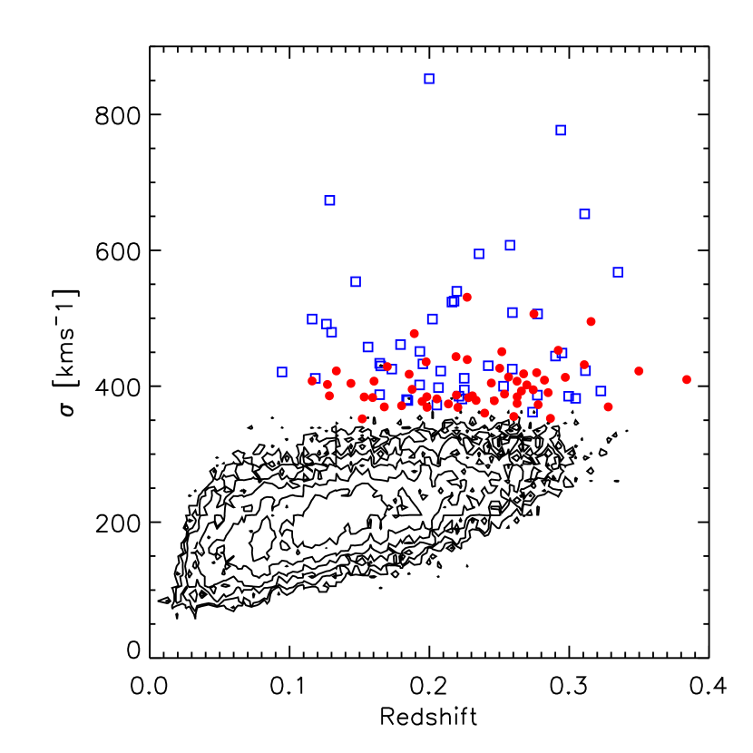
Figure 1.— Velocity dispersions of early-type galaxies as a function of redshift. Contours, spaced in factors of two from the maximum, represent the distribution of objects in the main sample, blue squares show the objects we think are superpositions, and red circles show objects for which the evidence for superposition is weakest.

The contours in Figure 1 show the distribution of velocity dispersions in our sample. (The convention is to report velocity dispersions which have been corrected to an aperture that is 1/8 times the half-light radius (e.g. Jørgensen, Franx & Kjærgaard 1995). We follow this convention, so the aperture corrected velocity dispersions reported below slightly larger than the measured values.) Because luminosity and velocity dispersion are correlated (Bernardi et al. 2003b show that $L\propto\sigma^{4}$) the objects with small velocity dispersions are likely to fall below the magnitude limit of our sample at higher redshifts. This accounts for the weak trend with redshift.

Of the main sample of objects represented by the contours, the spectroscopic pipeline reports that 105 have velocity dispersions $\sigma>350$ km s^-1. These estimates assume that the spectrum really is that of a single object. In Appendix A.1, we argue that the likelihood of a superposition which is sufficiently close that the photometry treats the blend as a single object is about one in every three hundred of the objects selected as early-types, so that some of the most distant luminous objects are likely to be superpositions. Therefore, we have performed our own estimates of the velocity dispersion for all these objects. Our analysis is described in some detail in Appendix A.2, where we conclude that most of the objects with $\sigma\gtrsim 500$ km s^-1 are actually superpositions. The small blue squares in Figure 1 show objects we identified as superpositions, and the small red circles show objects for which the evidence for superposition is less compelling.

Tables 1 and 2 list some of the important measured parameters of these objects. For objects which are not obvious superpositions Table 1 provides the object name, redshift, absolute $r-$band magnitude, restframe model $g-r$ color, $r-$band size, aperture corrected velocity dispersion and associated measurement errors. The magnitudes and sizes we use are those which come from the SDSS pipeline fits of a deVaucoleur’s profile to the surface-brightness distribution. In addition, the Table reports the S/N ratio of the spectrum, and for objects with S/N $\geq 18$, it reports the Mg₂ line-strength (estimates at lower S/N are very unreliable). These values are used in Section 4, which describes the results of an additional test of superposition. An asterix has been placed after the S/N values of all objects for which the evidence for superposition is weakest. These objects show little irregularity in imaging and little asymmetry in the cross-correlation function—they may well be single objects.

Table 2 provides analogous information for the objects which are almost certainly superpositions. For these objects, the measured parameters of the blend are almost certainly not those of the individual components, so we have chosen to not report the measurement errors (which are similar in magnitude to those in Table 1). However, we have included an estimate of the line-of-sight separation (in km s^-1) between the two components, obtained from the analysis described in Appendices A.2 and A.3.

Figure 1 shows fields which are a few arcseconds on a side (for reference, the angular diameter distance corresponding to one arcsecond at $z=0.3$ is $4.4h_{70}^{-1}$kpc), and slightly larger fields, $\sim 1$′ on a side, centered on each object which we did not classify as a superposition. (This larger scale is close to the minimum spacing between SDSS fibers, 55″, so, typically, only the central object in the field will have an SDSS spectrum, even if others satisfied the magnitude limit.) The figure also shows the result of two different techniques for estimating the velocity dispersion, as well as sections of the spectra of these objects, with the best-fitting template spectrum superimposed. In these figures, and these figures only, we show the measured velocity dispersion, before correcting to an aperture of $r_{e}/8$, since it is these measured values which are altered by superposition. Clearly, some of our objects are in relatively crowded fields, whereas others are rather isolated. A similar analysis of the objects classified as superpositions is shown in Figure 2. (The electronic version of this article shows similar figures for all the objects in our sample; only a few representative examples are presented here.)

3. Normal or Anomalous?

We have checked if the objects which are not obvious superpositions are a distinct population. Evidence that they are not substantially different from the bulk of early-type galaxies is presented in Figure 2. In each panel, contours represent the full early-type galaxy sample, blue squares represent the objects we identified as superpositions, and red circles represent objects which could be either singles or doubles. Error bars indicate the uncertainty in the measurements of the velocity dispersions, sizes, masses, and colors (in some cases they are smaller than the dimensions of the symbols; for clarity, and to illustrate the magnitude of the typical color error, we have only shown errors for some of the objects). The solid line in the top left panel shows the Fundamental Plane relation reported by Bernardi et al. (2003c); although this fit is based on old photometric and spectroscopic reductions, it’s slope provides a good description of the new data. Solid lines in the other panels show fits to the other scaling relations derived for the full early-type sample. Following Bernardi et al. (2003b,c), the luminosities and colors have been corrected for evolution (the correction is $0.85z$ to $M_{r}$ and $0.3z$ to $M_{g}-M_{r}$), and the fits correct for the effect of the magnitude limit of the SDSS.

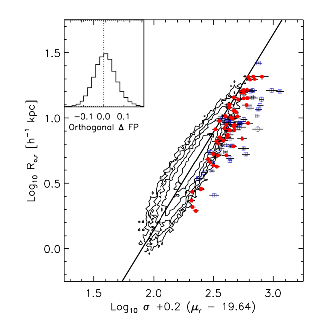
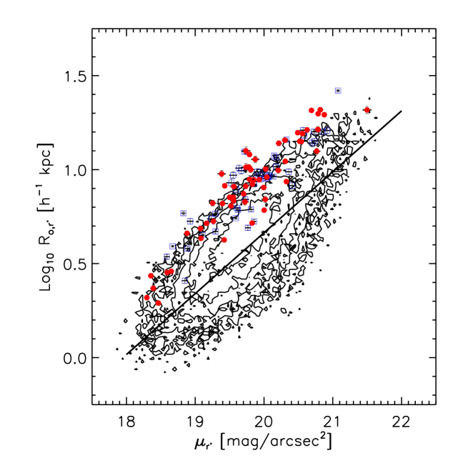
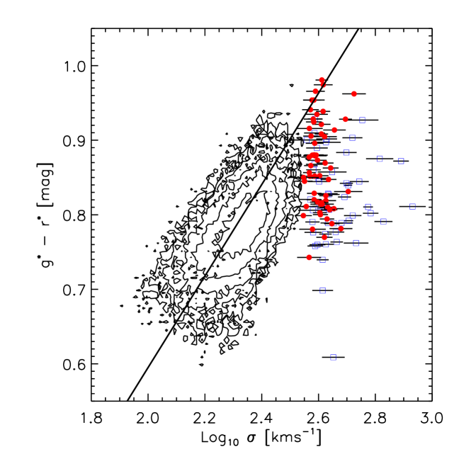
Figure 2.— Location of our sample of objects (red circles) with respect to the Fundamental Plane, the mass-luminosity relation, the size-surface brightness relation, the size-luminosity relation, the color-$\sigma$ and luminosity-$\sigma$ relations. Luminosities and colors have been corrected for evolution (following Bernardi et al. 2003b). Velocity dispersions have been corrected for aperture effects. Contours represent normal early-type galaxies, blue squares represent objects we are quite sure are superpositions, and red circles represent objects which could be either singles or doubles.

The objects with $\sigma>350$ km s^-1 which are not obvious doubles (red circles) clearly are extremes: they outline the high-mass border of the mass versus luminosity relation (top right panel), and they have the smallest sizes and the largest velocity dispersions for their luminosities (middle right and bottom right). However, although they outline the borders of these relations, they are not clear outliers. They also outline the borders of the Fundamental Plane (top left) and the size–surface-brightness (middle left) relations, but they are not outliers. In addition, although they are amongst the reddest objects (bottom left), they are not redder than extrapolation of the color–$\sigma$ relation from smaller $\sigma$ would suggest. In fact, these objects tend to lie slightly blueward of this relation, but again, they are not outliers. These objects appear to simply be the high velocity dispersion tail of the early-type galaxy population. The next section presents more evidence that many of these objects are not superpositions.

In contrast, the objects classified as superpositions (blue squares) are clear outliers from some of the scaling relations. In particular, they are offset towards extremely small sizes from the Fundamental Plane relation (top left). They also tend to be clear outliers from the mass versus luminosity relation, being offset towards very large mass values (top right). However, in the other scaling relations, they are not obviously different from the large-$\sigma$ objects which are not obvious superpositions, although they tend to scatter even more towards the bluer end of the color-$\sigma$ relation. In most cases, the offset from the scaling relations is removed if one assumes that because of the superposition, the correct position of the symbol is approximately given by making the luminosity fainter by a factor of two, decreasing the velocity dispersion by a factor of between 1.4 and 2 as well, but leaving the color unchanged. (The factor of two in luminosity is easily justified, since if the luminosity ratio was extreme, the light from the fainter member of the pair would simply not be noticed. The factor of 1.5 or so in $\sigma$ is less straightforward; it is approximately what we find in our analysis of the superpositions in Appendix A.)

Perhaps the most striking feature of the different panels is that the objects which were not obvious doubles are also not obvious outliers from the scaling relations defined by the main early-type sample (although they do define the borders). In constrast, the objects we classified as doubles are more distant outliers—even though these scaling relations played no role in the determining whether an object was a single or a double. Clearly, identifying outliers from the Fundamental Plane and mass versus luminosity relations is a simple way of searching for superpositions.

Figure 3.— Velocity dispersion correction factor for various indices, calibrated using the models of Bruzual & Charlot (2003). This correction does not depend on metallicity.

4. On rejecting the superposition hypothesis

The previous section argued that doubles were relatively easy to identify, since they were obvious outliers from the scaling relations defined by the bulk of the population. But is there a way to reject the superposition hypothesis? In this section, we argue that this may be possible. The idea is that if superposition tends to increase the estimated velocity dispersion, then it probably also changes the infered absorption line-strengths in the spectrum. For instance, if two identical galaxies have a small line-of-sight separation, and all lines in the spectra of the individual objects have Gaussian profiles, then the spectrum of the superposition will have lines which are broader (hence increasing the infered $\sigma$). Roughly speaking, line-strengths are related to the ratio of the flux in the line-center to the flux in the wings, so the superposition will have a smaller line-strength. Therefore, superpositions may be obvious outliers from any linestrength$-\sigma$ relations defined by the bulk of the population.

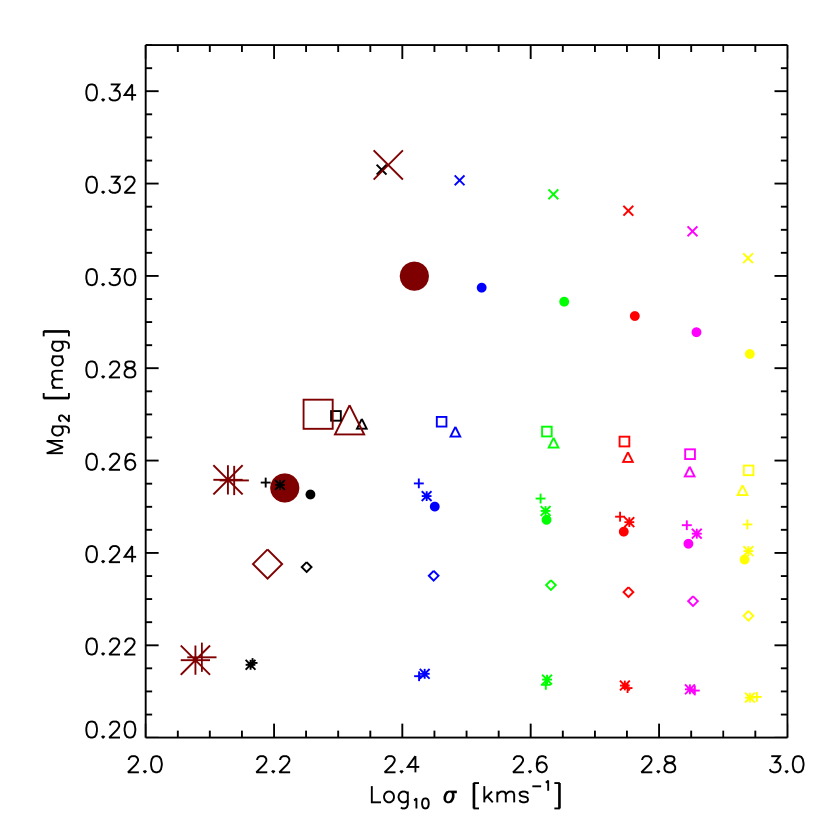
Figure 4.— Effect of superposition on estimated velocity dispersions $\sigma$ and Mg₂ line-strengths; the superposition is assumed to be of otherwise identical objects. Large (brown) symbols show the values of $\sigma$ and Mg₂ for a single component (i.e., line-of-sight separation $\Delta z=0$); small symbols show how the estimated values change as the velocity separation between the two components increases in steps of 200 km s^-1: $\sigma$ increases and Mg₂ decreases with increasing separation.

With this in mind, we have measured various indicators of the chemical compositions of these objects: the Lick indices Mg$b$ and $\langle{\rm Fe}\rangle$ are sensitive to both age and metallicity, their ratio is an indicator of the relative abundances of $\alpha$-elements, $C_{2}4668$ is also sensitive to age and metallicity, and H$\delta_{\rm A}$ and H$\gamma_{\rm F}$ are indicators of more recent star formation (Worthey & Ottaviani 1997). It is conventional to report the measured value after correction for the effects of velocity dispersion and aperture: the correction factors for velocity dispersion are shown in Figure 3. Since $\sigma$ may be large, the corrections may also be large for some of the indices (e.g. the two iron lines Fe5270 and Fe5335). However, the correction for Mg₂ is small; less than ten percent even when $\sigma\sim 600$ km s^-1. For this reason, we will use it in what follows. In addition, the Mg₂ index can be measured accurately also for relatively low S/N spectra.

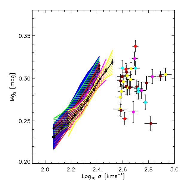
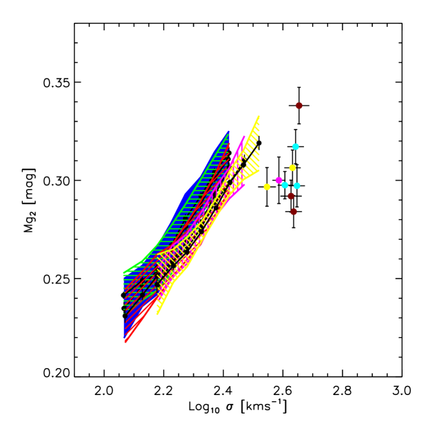
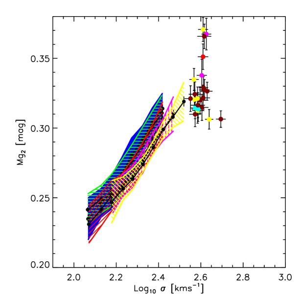
Figure 5.— Comparison of Mg${}_{2}-\sigma$ correlation defined by the bulk of the population (hashed regions), with the locus of points defined by the objects with strong, intermediate, and weak evidence for superposition (top, middle and bottom panels). Superpositions should be located down and to the right of the true relation—this is true of most of the objects in the top panel. By this measure, objects in the bottom panel may well be single massive galaxies.

To study the effect of superposition on $\sigma$ and Mg₂, we have summed two identical spectra (chosen from among the high S/N composite spectra described in the next paragraph), with redshift separations $\Delta z$, and computed the velocity dispersion and Mg₂ strengths using the usual methods. Figure 4 shows the results of this exercise as $c\Delta z$ is varied from 0 to 1200 km s^-1, in steps of 200 km s^-1. Large (brown) symbols show $\sigma$ and line-strength when $\Delta z=0$ (so the values are the same as of the single component), and small symbols show the estimated $\sigma$ and Mg₂ value as the separation between the pair increases. Increasing the separation tends to increase $\sigma$ and decrease Mg₂, as expected.

Our use of identical spectra to illustrate this effect is less unrealistic than one might have thought. This is because the estimated velocity dispersion of the blend depends not only on the velocity dispersion and line-of-sight separation of the components, but also on the flux-ratio of the two components. Hence, the two components should have similar fluxes, and, being at approximately the same redshift, they should have approximately the same luminosities. However, velocity dispersion and luminosity are correlated: in this sample, $L\propto\sigma^{4}$ (Bernardi et al. 2003b). If the individual components both lie on this $\sigma-L$ relation, then if the two values of $\sigma$ differ by more than a factor of $\sim 1.8$, the flux-ratio will be larger than $\sim 10$, and the smaller component is unlikely to have a significant effect. Thus, if we detect superpositions from the spectra, it is likely that the spectra of the two components will have relatively similar velocity dispersions, and hence relatively similar absorption features. This expectation is borne out by the fact that, of the systems which were clear superpositions, the estimated velocity dispersions of the two components tend to be similar (Figures 2). Thus, even in the general case, the estimates of the effect of superposition on the Mg${}_{2}-\sigma$ relation shown in Figure 4 are likely to be qualitatively correct.

To see if the Mg${}_{2}-\sigma$ relation provides a reasonable diagnostic of superposition, we must compare the location of the systems with large $\sigma$ in the Mg${}_{2}-\sigma$ plane, with the region populated by the main sample. To define the Mg${}_{2}-\sigma$ relation associated with the bulk of the early-type population, we used composite spectra constructed as described in Bernardi et al. (2005). Each composite has S/N $\sim 100$ or larger (making the estimate of the line-strength more reliable), and is made by summing the spectra of galaxies with similar magnitudes, sizes, velocity dispersions and redshifts.

The different panels of Figure 5 all show the Mg${}_{2}-\sigma$ relation traced by the main population: black solid lines show the weighted mean of the index strength, hashed regions show the rms scatter around these mean values in the different redshift bins (blue, green, red, magenta and yellow bands show results for $0.04<z<0.07$, $0.07<z<0.09$, $0.09<z<0.12$, $0.12<z<0.15$, and $0.15<z<0.20$; colors of the filled circles in the different panels also indicate these same redshift bins. Cyan and brown symbols represent galaxies at even higher redshifts: $0.2\leq z<0.25$ and $z\geq 0.25$, respectively). Notice that the Mg${}_{2}-\sigma$ relation evolves: at fixed $\sigma$, Mg₂ decreases with increasing $z$. This is consistent with previous work (e.g. Bernardi et al. 2003d). In the top panel, the filled circles with error bars represent those objects classified as superpositions with S/N $\geq 18$ (it is difficult to make reliable estimates at smaller S/N ratios). The previous figure suggests that superpositions should lie down and to the right of the true relation: the filled circles do indeed show such an offset. The filled circles in the middle panel show those objects which are not obvious superpositions, but do still have odd features in their spectra. While the objects which lie below the Mg${}_{2}-\sigma$ relation are probably superpositions, the ones which lie close to the relation may well be single objects. The bottom panel shows a similar analysis applied to the objects for which the evidence for superposition is weakest: neither the images nor the spectra showed compelling evidence for superposition. These objects tend to lie on or slightly above the mean Mg${}_{2}-\sigma$ relation; the results of Figure 4 suggest that they are very unlikely to be superpositions. These objects may well be some of the most massive galaxies in the Universe.

5. Discussion

We searched the SDSS database for a population of objects with anomalously large velocity dispersions, and found $\sim 100$ objects with estimated dispersions in excess of 350 km s^-1. Of these, about half appear to be superpositions (so the reported velocity dispersion is unrealistic); in many cases, the evidence for superposition comes not from the images but from the spectra (Figure 2). These superpositions are rare: analytic and Monte-Carlo analyses in Appendix A suggest that one in every three hundred objects should have a neighbor within one arcsec. Moreover, of alignments closer than one arcsec, not more than ten percent are expected to be from objects in different groups. If the superpositions we see really are in the same halos, then our estimates of the line-of-sight separations imply halo masses of order $5\times 10^{14}h^{-1}M_{\odot}$.

The large-$\sigma$ objects which are not obviously superpositions populate the tails of the scaling relations defined by the bulk of the early-type galaxy population (quantified by Bernardi et al. 2005), but they are not distant outliers from these relations (Figures 2 and 5). Moreover, if only half of these objects turn out to be superpositions, and the other half are indeed single galaxies, then the abundance of singles is not inconsistent with the number expected by extrapolation of the observed abundance of smaller systems (from Sheth et al. 2003).

If these large-$\sigma$ objects are indeed massive galaxies, and the velocity dispersions do reflect virial equilibrium motions, then it might be worth searching for evidence of gravitational lensing around these objects: they would have Einstein radii $4\pi(\sigma/c)^{2}(d_{\rm ls}/d_{\rm os})\sim 2.3\arcsec(d_{\rm ls}/d_{\rm os})/(1/2)$ $(\sigma/400~{}{\rm km~{}s}^{-1})^{2}$. If they host black holes whose masses fall on the same mass-velocity dispersion relation as is seen locally, $M_{\rm BH}/10^{9}M_{\odot}=2\,(\sigma/400~{}{\rm km~{}s}^{-1})^{4}$ (Gebhardt et al. 2000; Ferrarese & Merritt 2000; Tremaine et al. 2002), then the black-holes are enormous indeed. In this case, it will be interesting to see if the light-profile shows any evidence of the black-hole in the center (e.g. Lauer et al. 2002) using HST. Because they are large and luminous, these objects should be relatively easy targets. Therefore, it should also be possible to measure spatially resolved velocity dispersions from ground-based facilities.

The superpositions are interesting in their own right. The abundance of strong gravitational lenses has been used to place limits on the geometry of the Universe (e.g. Mitchell et al. 2004). However, the observed distributions of image multiplicities, separations and flux ratios are difficult to reconcile with single-component lens models. This has led to some interest in the properties of lenses with multiple components (e.g., Rusin & Tegmark 2001; Cohn & Kochanek 2004). Since early-type galaxies are expected to be the dominant lens population, the distribution of pair separations and velocity dispersions in our catalog of superpositions can be used to incorporate realistic lens pairs into models of binary-lenses. This is the subject of work in progress.

And finally, in principle, the number and spatial distribution of close superpositions contains information about the time-scale of mergers. In this regard, it is interesting that a number of the objects in our sample appear to have slightly peculiar morphologies. If this reflects a recent merger, then it is interesting to recall that none of the spectra in our sample show strong emission lines. Therefore, it may be that these objects are the low redshift analogs of the red interacting galaxies seen in the GOODS survey (Somerville et al. 2003). Or perhaps they are fossil groups of the sort discussed by Vikhlinin (1999) and Jones et al. (2003). Follow-up observations of these objects is ongoing.

We thank Karl Gebhardt for encouragement.

Funding for the creation and distribution of the SDSS Archive has been provided by the Alfred P. Sloan Foundation, the Participating Institutions, the National Aeronautics and Space Administration, the National Science Foundation, the U.S. Department of Energy, the Japanese Monbukagakusho, and the Max Planck Society. The SDSS Web site is http://www.sdss.org/.

The SDSS is managed by the Astrophysical Research Consortium (ARC) for the Participating Institutions. The Participating Institutions are The University of Chicago, Fermilab, the Institute for Advanced Study, the Japan Participation Group, The Johns Hopkins University, the Korean Scientist Group, Los Alamos National Laboratory, the Max-Planck-Institute for Astronomy (MPIA), the Max-Planck-Institute for Astrophysics (MPA), New Mexico State University, University of Pittsburgh, Princeton University, the United States Naval Observatory, and the University of Washington.

Table 1Physical parameters and median errors of the objects in our sample which are not obvious superpositions. Estimates of Mg₂ were only made if S/N $\geq 18$. Asterisk in final column denotes objects for which the evidence for superposition is weakest.

name	$z$	$M_{r}$	$e_{M}$	$g-r$	$e_{g-r}$	log${}_{10}R$	$e_{R}$	$\sigma$	$e_{\sigma}$	Mg2	$e_{\rm{Mg}_{2}}$	$S/N$
		[mag]	[mag]	[mag]	[mag]	[kpc]	[kpc]	kms-1	kms-1	[mag]	[mag]
SDSS J094035.8+022950.0	0.15196	$-$22.90	0.02	0.80	0.02	0.93	0.01	352	29	0.297	0.010	18
SDSS J112626.6+003620.7	0.28655	$-$23.66	0.04	0.85	0.06	1.32	0.02	352	53	–	–	12
SDSS J083551.2+392621.7	0.26035	$-$23.96	0.02	0.84	0.02	1.13	0.01	355	29	0.321	0.009	19*
SDSS J013431.5+131436.4	0.23949	$-$23.32	0.03	0.81	0.04	1.00	0.02	360	37	–	–	13*
SDSS J162332.4+450032.0	0.19827	$-$23.23	0.02	0.88	0.02	0.90	0.01	368	28	–	–	16*
SDSS J132808.5+031817.1	0.22034	$-$23.26	0.03	0.74	0.03	1.09	0.02	369	41	–	–	13
SDSS J010803.2+151333.6	0.16773	$-$23.45	0.01	0.86	0.02	1.04	0.01	369	22	0.335	0.008	21*
SDSS J083445.2+355142.0	0.32787	$-$23.91	0.03	0.92	0.05	1.18	0.02	371	52	–	–	13
SDSS J131419.7$-$012726.0	0.18011	$-$24.06	0.01	0.85	0.01	1.20	0.01	371	23	0.320	0.007	24*
SDSS J091944.2+562201.1	0.27775	$-$23.96	0.02	0.94	0.03	1.20	0.01	373	30	0.324	0.009	19*
SDSS J155944.2+005236.8	0.21356	$-$23.65	0.02	0.87	0.03	0.90	0.01	373	22	0.314	0.008	22*
SDSS J135602.4+021044.6	0.26271	$-$24.11	0.02	0.91	0.04	1.30	0.01	374	29	0.310	0.009	19*
SDSS J075923.1+274148.3	0.19477	$-$23.03	0.02	0.95	0.01	0.82	0.01	376	30	–	–	17*
SDSS J141341.4+033104.3	0.24639	$-$23.53	0.03	0.88	0.04	0.99	0.02	379	33	–	–	16*
SDSS J112842.0+043221.7	0.20533	$-$22.99	0.03	0.93	0.04	0.83	0.02	381	34	–	–	14*
SDSS J124134.3+604147.2	0.23336	$-$23.10	0.02	0.78	0.03	0.84	0.01	381	47	–	–	14
SDSS J093124.4+574926.6	0.22792	$-$22.94	0.03	0.92	0.04	0.69	0.02	383	27	–	–	16*
SDSS J103344.2+043143.5	0.15939	$-$22.32	0.02	0.95	0.02	0.72	0.01	383	41	–	–	11
SDSS J221414.3+131703.7	0.15335	$-$22.02	0.03	0.82	0.01	0.37	0.02	384	28	0.321	0.008	20*
SDSS J225331.3+130116.9	0.19812	$-$23.26	0.02	0.83	0.02	0.85	0.01	384	26	0.313	0.009	19*
SDSS J120011.1+680924.8	0.26275	$-$24.07	0.02	0.88	0.03	1.18	0.01	385	34	0.316	0.009	19*
SDSS J154651.5+570736.2	0.12845	$-$22.28	0.02	0.85	0.01	0.62	0.01	385	24	0.300	0.012	22
SDSS J211019.2+095047.1	0.23073	$-$23.85	0.02	0.90	0.03	0.99	0.01	386	32	0.314	0.009	19*
SDSS J160239.1+022110.0	0.21930	$-$22.93	0.03	0.88	0.03	0.73	0.02	386	41	–	–	10
SDSS J154017.3+430024.5	0.25370	$-$23.77	0.02	0.97	0.03	1.14	0.01	388	36	–	–	16*
SDSS J111525.7+024033.9	0.28489	$-$23.52	0.04	0.88	0.04	0.91	0.02	391	44	–	–	13
SDSS J130615.8+600125.2	0.26580	$-$23.16	0.03	0.93	0.05	0.84	0.02	392	44	–	–	12
SDSS J145506.8+615809.7	0.27422	$-$24.45	0.02	0.87	0.02	1.32	0.01	394	36	0.320	0.010	18*
SDSS J235354.1$-$093908.3	0.18764	$-$22.39	0.02	0.82	0.04	0.44	0.02	395	27	–	–	16*
SDSS J082216.5+481519.1	0.12705	$-$21.52	0.02	0.80	0.02	0.29	0.01	402	28	0.338	0.012	19*
SDSS J124609.4+515021.6	0.26965	$-$24.07	0.02	0.85	0.02	1.12	0.01	402	35	0.315	0.009	18*
SDSS J204712.0$-$054336.7	0.14386	$-$22.49	0.02	0.80	0.01	0.78	0.01	404	32	–	–	17
SDSS J085738.8+561121.0	0.24427	$-$23.21	0.04	0.81	0.04	0.82	0.03	404	25	0.298	0.007	21
SDSS J151741.7$-$004217.6	0.11610	$-$21.87	0.02	0.82	0.01	0.32	0.01	407	27	0.351	0.009	24*
SDSS J082646.7+495211.5	0.16037	$-$22.29	0.02	0.91	0.02	0.46	0.01	408	26	0.371	0.009	21*
SDSS J011613.8$-$092625.2	0.26262	$-$23.35	0.02	0.92	0.06	0.88	0.02	408	39	0.322	0.009	18*
SDSS J084257.5+362159.3	0.28227	$-$24.28	0.02	0.98	0.03	1.28	0.01	409	31	0.329	0.008	21*
SDSS J204642.1+000507.7	0.25658	$-$23.42	0.03	0.97	0.06	0.82	0.02	413	35	0.366	0.009	19*
SDSS J171328.4+274336.6	0.29718	$-$24.28	0.02	0.94	0.04	1.08	0.01	413	27	0.327	0.007	22*
SDSS J134126.7+013641.1	0.38403	$-$24.08	0.03	0.81	0.07	0.86	0.02	414	49	–	–	16
SDSS J224248.8+135430.8	0.18549	$-$22.28	0.02	0.77	0.02	0.47	0.01	417	30	–	–	17
SDSS J114747.0+034838.7	0.26737	$-$23.12	0.05	0.90	0.07	0.82	0.03	419	62	–	–	12
SDSS J135533.4+515617.8	0.27669	$-$23.79	0.02	0.87	0.04	1.13	0.01	420	43	–	–	14
SDSS J133724.7+033656.5	0.13343	$-$22.68	0.01	0.83	0.01	0.63	0.01	422	31	0.367	0.011	19*
SDSS J031539.2$-$081014.3	0.34977	$-$24.34	0.04	0.82	0.09	1.06	0.02	423	38	0.292	0.008	22
SDSS J104056.4$-$010358.7	0.25026	$-$24.27	0.02	0.79	0.02	1.30	0.01	426	30	0.326	0.006	25*
SDSS J141922.4+011457.8	0.16984	$-$23.37	0.02	0.81	0.02	0.95	0.01	428	30	0.306	0.009	19
SDSS J133046.1+585049.9	0.31075	$-$23.92	0.03	0.85	0.03	1.03	0.02	432	38	0.284	0.008	20
SDSS J161541.3+471004.3	0.19766	$-$22.99	0.02	0.81	0.00	0.66	0.01	435	21	0.306	0.007	24*
SDSS J132356.8+001049.8	0.22705	$-$23.44	0.02	0.86	0.02	0.95	0.01	439	32	0.317	0.009	20
SDSS J111505.5+051833.6	0.21901	$-$23.01	0.02	0.79	0.04	0.71	0.01	443	31	0.297	0.011	18
SDSS J161615.5+435559.5	0.25178	$-$23.33	0.02	0.81	0.04	0.85	0.01	451	40	0.338	0.009	19
SDSS J232331.4$-$102551.7	0.29211	$-$23.79	0.03	0.91	0.08	0.99	0.02	453	46	–	–	17
SDSS J141102.6+030805.7	0.18917	$-$22.75	0.03	0.78	0.02	0.84	0.02	477	48	–	–	12
SDSS J032834.7+001050.1	0.31557	$-$23.89	0.04	0.93	0.07	1.02	0.02	494	28	0.306	0.006	30*
SDSS J223859.6+004041.4	0.27472	$-$23.47	0.03	0.83	0.04	0.86	0.02	507	66	–	–	13
SDSS J010354.1+144814.1	0.22693	$-$23.25	0.02	0.96	0.06	0.97	0.01	529	58	–	–	16

Table 2Physical parameters of the objects in our sample which are almost certainly superpositions. An estimate of the separation along the line-of-sight is also provided. For these objects, the measured parameters of the blend are almost certainly not those of the individual components, so the measurement errors are not reported.

name	$z$	$M_{r}$	$g-r$	log${}_{10}R$	$\Delta cz$	$\sigma$	Mg2	$S/N$
		[mag]	[mag]	[kpc]	[km s-1]	[km s-1]	[mag]
SDSS J150821.4$-$021637.9	0.27380	$-$23.31	0.90	0.97	900	361	–	12
SDSS J021046.9+143448.4	0.20529	$-$22.91	0.82	0.74	600	371	–	15
SDSS J150128.7+033630.4	0.18459	$-$23.93	0.79	1.18	–	379	0.278	20
SDSS J091545.5+505424.4	0.18364	$-$23.48	0.81	0.97	900	380	0.264	21
SDSS J163005.3+463611.2	0.22330	$-$23.19	0.78	0.90	750	380	–	16
SDSS J095937.6+031001.7	0.30452	$-$23.87	0.86	0.99	750	382	0.297	22
SDSS J022433.2$-$073111.0	0.27716	$-$23.58	0.93	1.03	600	385	0.262	23
SDSS J145710.1+604207.2	0.22112	$-$23.32	0.87	0.95	1200	385	–	16
SDSS J144525.1+591327.5	0.29959	$-$23.65	0.91	1.16	–	386	–	15
SDSS J140836.5+613108.0	0.16440	$-$22.57	0.76	0.58	600	387	0.285	20
SDSS J142437.2+000835.6	0.32261	$-$23.97	0.89	1.01	–	392	0.302	18
SDSS J135331.2+533430.7	0.22495	$-$23.55	0.76	1.00	450	394	0.312	20
SDSS J173820.0+551638.8	0.20645	$-$22.58	0.85	0.51	450	398	–	17
SDSS J152333.3+450335.7	0.25304	$-$23.86	0.84	1.20	–	400	–	14
SDSS J215541.9+123128.6	0.19300	$-$24.62	0.81	1.43	600	401	0.296	21
SDSS J120439.0+601211.2	0.11842	$-$22.73	0.74	0.66	750	411	0.253	30
SDSS J231543.5$-$000511.6	0.22490	$-$22.94	0.70	0.79	299	411	–	15
SDSS J153603.4+003749.3	0.09460	$-$22.69	0.77	0.74	600	420	0.311	29
SDSS J104940.3+050307.1	0.31160	$-$23.87	0.90	0.97	750	422	0.291	19
SDSS J122051.1+533436.2	0.20808	$-$23.19	0.76	0.97	600	423	–	16
SDSS J020556.7+000056.6	0.17308	$-$22.26	0.81	0.73	600	423	–	15
SDSS J142543.5+620500.0	0.25925	$-$23.60	0.90	1.14	450	425	0.307	20
SDSS J141557.6+031821.2	0.16520	$-$23.26	0.79	0.96	600	429	0.303	19
SDSS J075527.6+360749.6	0.24205	$-$22.93	0.83	0.82	750	430	–	16
SDSS J102618.9+492119.2	0.19533	$-$23.08	0.83	0.75	600	433	0.289	18
SDSS J214141.6+011146.9	0.16447	$-$22.67	0.81	0.78	750	433	–	17
SDSS J074224.6+305345.6	0.29015	$-$23.36	0.86	0.97	–	444	–	12
SDSS J021148.2+001639.7	0.29476	$-$23.46	0.61	0.88	450	449	0.289	19
SDSS J114634.4+022147.5	0.19317	$-$22.86	0.79	0.77	600	451	–	17
SDSS J014157.5$-$010626.3	0.15613	$-$23.32	0.78	0.96	750	457	0.299	20
SDSS J133153.5+031750.5	0.17934	$-$23.36	0.76	0.95	750	461	0.311	22
SDSS J153228.9+023916.5	0.13003	$-$21.79	0.79	0.41	570	479	0.261	18
SDSS J104907.2+551314.9	0.12631	$-$23.48	0.82	0.95	900	491	0.323	27
SDSS J000740.4+144506.7	0.11610	$-$22.85	0.84	0.59	750	498	0.337	32
SDSS J152242.7+574009.5	0.20218	$-$24.04	0.88	1.16	1050	498	0.312	20
SDSS J115514.0$-$012041.1	0.27735	$-$23.60	0.84	1.15	750	506	–	12
SDSS J155614.1+484706.1	0.25938	$-$23.45	0.79	0.71	1050	510	0.290	22
SDSS J090321.9+520607.6	0.21608	$-$22.65	0.90	0.66	1050	524	0.288	21
SDSS J150550.3+042909.3	0.21763	$-$23.77	0.80	1.05	1200	526	0.284	20
SDSS J130543.9+674615.6	0.21956	$-$22.91	0.76	0.92	900	541	–	13
SDSS J131616.2+051403.7	0.14727	$-$22.42	0.84	0.72	–	554	0.286	19
SDSS J094436.5+614411.5	0.33489	$-$23.69	0.93	0.96	900	566	–	13
SDSS J080413.1+372737.9	0.23550	$-$23.47	0.81	1.01	900	594	0.272	18
SDSS J162255.0+455514.7	0.25767	$-$23.72	0.80	1.07	1050	607	0.295	22
SDSS J133035.4+590117.3	0.31102	$-$24.00	0.88	1.18	1350	654	0.247	19
SDSS J103836.6+011749.4	0.12871	$-$23.72	0.79	1.20	1200	673	0.302	27
SDSS J080234.9+362100.9	0.29396	$-$24.37	0.87	1.08	1350	778	0.302	30
SDSS J021515.5+005823.7	0.19985	$-$23.59	0.81	0.77	1350	852	0.304	23

Appendix A A. Superpositions

A.1. A.1 Likelihood of superpositions

In the main text we stated that a number of our objects were superpositions, even though the SDSS photometric pipeline classified them as single objects. In this section, we make a number of estimates of the likelihood of having a superposition with image separations of order 1 arcsec: this is a convenient number as it happens to be approximately the size of the typical SDSS seeing disk, and it is slightly smaller than the 1.5 arcsecond radius of an SDSS fiber.

A simple but inaccurate estimate follows from ignoring the fact that galaxies cluster. If the galaxies were Poisson-distributed, then the typical number of galaxies within a small angle $\theta$ would be $\bar{N}=\bar{n}\pi\theta^{2}$, where $\bar{n}$ is the mean density of galaxies on the surface of the sky. For a Poisson distribution, the probability that a region of size $A$ which is centred on a randomly chosen galaxy contains at least one other galaxy is $p(>0|A)=1-{\rm exp}(-\bar{N})$, where $\bar{N}$ denotes the typical number of galaxies in regions of size $A$. We are interested in regions which are typically an arcsecond in radius (recall that the diameter of an SDSS fiber is 3 arcsec); we will argue below that this means $\bar{N}\ll 1$, so $p(>0|A)\approx\bar{N}$. To justify this, we must estimate $\bar{n}$.

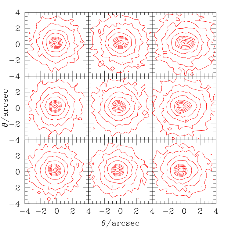
Figure 1.— Simulations of two-component images. Each component is a deVaucoleur profile with half light radius 2″, the effects of seeing are modeled by a symmetric Gaussian with FWHM = 1.5″, and the photon counts are binned in square pixels which are 0.4″on a side. Together, the two components sum to $r=17.5$ mags. Panels from left to right show what happens as the separation between the objects increases from 0.4 to 0.8 to 1.2″, and from top to bottom show brightness ratios of 1, 2.5 and 10 (the brighter component is on the left). Contours show isophotes which are 0.9, 0.8, 0.7, 0.6, 0.5, 0.25, 0.125, 0.0625 and 0.03125 times the maximum. Seeing limits evidence for superposition from the photometry to angular separations $\gtrsim$1″, and this minimum scale increases if the brightnesses of the two components are very different.

In principal, the superposed galaxy could be any morphological type and any intrinsic luminosity, since the magnitude limit only constrains the combined luminosities of the blend. In practice, we would only really notice the superposition if the apparent brightnesses do not differ by more than a factor of ten (e.g. Figure 1). Moreover, if the second object showed emission lines, the blend would probably have been excluded from the sample. Therefore, as a first simple estimate of the $\bar{n}$ we are after we use the total number density of early-types, whatever their luminosity. Since we see $\sim 30,000$ galaxies in $\sim 2200$ sq. deg., there are about $10^{-6}$ galaxies per square arcsec, so the probability of overlap is $\sim(\pi\times 10^{-6})(\theta/{\rm arcsec})^{2}$; we would expect to find one pair separated by less than 1 arcsec for every few hundred thousand galaxies. This is significantly smaller than we think we find, presumably because by ignoring clustering, we have underestimated the number of close pairs.

To approximately account for clustering, suppose that the spatial correlation function is $\xi(z,p)=[r_{0}^{2}/(z^{2}+p^{2})]^{\gamma/2}$, where $z$ and $p$ denote comoving distances along and perpendicular to the line of sight. Provided $\gamma>1$, the number of excess pairs at projected distance $p$ is $w(p)=\int dz\,\xi(z,p)=g(\gamma)\,r_{0}\,(r_{0}/p)^{\gamma-1}$ where $g(\gamma)=\sqrt{\pi}\Gamma[(\gamma-1)/2]/\Gamma[\gamma/2]$. The typical number of extra pairs within projected comoving distance $p$ of a randomly chosen galaxy is

$$\bar{N}_{\rm cl}(<p)=\bar{n}\,2\pi\int{\rm d}p\,pw(p)=\bar{n}\,{2\pi p^{2}\,w(p)\over 3-\gamma}.$$ (A1)

For a sample of galaxies which is similar to our early-type sample, Budavari et al. (2003) find that $\gamma=2$ and $r_{0}=8h^{-1}$Mpc (their reddest, most luminous sample). If we approximate $p\approx(cz/H)\,\theta$, then

$$\bar{N}_{\rm cl}(<\theta|z)\approx 0.0043\left({\bar{n}\,{\rm Mpc}^{3}\over 0.001h^{3}}\right)\left({r_{0}\,h\over 8\,{\rm Mpc}}\right)^{2}\left({z\over 0.22}\right)\left({\theta\over{\rm arcsec}}\right)$$ (A2)

Note that the number of random pairs on these scales, $\sim\pi\times 10^{-6}\,(\theta/{\rm arcsec})^{2}$, is substantially smaller, so can safely be neglected.

Integrating over the range of observed redshifts will only modify this estimate slightly. For instance, the observed redshift distribution is well approximated by $dz\,dN/dz\propto 2\,(dz/z)\,(z/z_{m})^{3}\exp[-(z/z_{m})^{2}]/\Gamma(3/2)$, with $z_{m}=0.11$, so

$$\int dz\,{dN\over dz}\,\bar{N}_{\rm cl}(<\theta|z)={2\over\sqrt{\pi}}\,\bar{N}_{\rm cl}(<\theta|z_{m}).$$ (A3)

Thus, this analysis suggests that about one in every four hundred objects will be a blend. Notice also that, at least on small scales, the number of blends increases as $\theta^{3-\gamma}$; for $\gamma=2$, the number scales linearly with the allowed angular separation between the blends.

This analysis assumes that $\xi$ is a power-law all the way down to vanishingly small scales. If $\xi$ is shallower on small scales, then the predicted number of superpositions is smaller, and scales approximately as $\theta^{3-\gamma_{\rm eff}}$, where $\gamma_{\rm eff}$ is the effective slope on scales of order 10 kpc (recall that 1″ at $z=0.3$ is 4.4 kpc).

To account more carefully for the effects of clustering and the magnitude limit is more complicated. We have chosen to do so by performing Monte-Carlo simulations as follows. Note that this analysis is not intended to be definitive—we only wish to demonstrate how more sophisticated models of the early-type galaxy distribution can yield substantially more information about the likelihood of superposition. Conversely, the fraction of superpositions constrain the various parameters of such Monte-Carlo models.

We start with the Very Large Simulation (VLS; Yoshida, Sheth & Diaferio 2001) of a $\Lambda$CDM cosmology. This simulation followed the evolution of $512^{3}$ particles in a $479h^{-1}$Mpc cube; the particle mass in the simulation is $6.86\times 10^{10}h^{-1}M_{\odot}$, so halos more massive than $\sim 1.3\times 10^{12}h^{-1}M_{\odot}$ are reasonably well represented by the simulation. A catalog of the positions and masses of the dark matter halos in this simulation has been made available by the Virgo consortium (http://www.mpa-garching.mpg.de/Virgo). We model the SDSS early-type galaxy distribution by populating the simulated halos with model galaxies in such a way that the luminosity function, and the luminosity dependence of clustering are approximately reproduced. In particular, Zehavi et al. (2005) studied the clustering of galaxies as a function of luminosity in the SDSS. Although they did not study clustering as a function of morphological type, we use some aspects of their results to guide the construction of our mock catalogs as follows.

We assume that the mean number of early-type galaxies increases with halo mass as $\langle N_{\rm gal}|M_{\rm halo}\rangle=1+M_{\rm halo}/23M_{\rm min}$ provided $M_{\rm halo}>M_{\rm min}$, and it is zero in lower mass haloes. The parameter $M_{\rm min}$ is chosen to match the number density of early-type galaxies reported by Bernardi et al. (2003b): in our case, $M_{\rm min}=1.5\times 10^{12}h^{-1}M_{\odot}$. With this prescription, about twenty percent of the galaxies are in halos which host at least one other galaxy. In all halos more massive than $M_{\rm min}$, we place the first galaxy at the halo centre, then draw a Poisson random number $N_{\rm sat}$ which has mean $M_{\rm halo}/23M_{\rm min}$ (a Poisson distribution for the satellite galaxies is motivated by the work of Kravtsov et al. 2004), and distribute the $N_{\rm sat}$ satellite galaxies around the halo centre so the resulting density run of galaxies resembles an NFW profile (Navarro et al. 1997).

To insure that the mock galaxy sample has the correct distribution of luminosities, we generate the Lognormal distribution which Bernardi et al. (2003b) find describes this early-type sample well. The results of Zehavi et al. (2005) suggest that the central galaxy in a halo is almost always substantially more luminous than the others, and that its luminosity increases monotonically with the mass of its host halo. In contrast, the distribution of satellite galaxy luminosities depends only weakly on parent halo mass. To incorporate such an effect into our mocks, we rank order the luminosities and the host halo masses, assign the brightest luminosity to the galaxy at the centre of the most massive halo, and work our way down the set of luminosities and halos, assigning successively fainter luminosities to central galaxies of host halos with ever lower masses. Once all central galaxies have been assigned luminosities, the fainter luminosities which remain are assigned to satellites without regard to the masses of the parent halos.

We then model the SDSS survey as a cone oriented in a random direction within the box, and compute angular positions, redshifts and apparent magnitudes for each simulated ‘galaxy’. In this way, we can simulate the chance of having a blend which would have been bright enough to satisfy the SDSS magnitude limit.

The simulation box is $L=479h^{-1}$Mpc comoving on a side, which means that observations out to $z\sim 0.16$ are straightforward to model. Since we would like to reach to redshifts of order 0.3, we surround the initial box by copies of itself, each rotated by a random angle, to avoid spurious projection effects. This is not ideal, particularly because the VLS halo catalogs are taken from a single snapshot at $z=0$, so our mock catalogs do not account for evolution along the lightcone. A similar analysis using the Hubble Volume lightcone outputs is only possible for halos more massive than $5\times 10^{13}h^{-1}M_{\odot}$. For these more massive halos, the VLS and Hubble Volume catalogs yield similar results, suggesting that evolution along the lightcone is not an important effect. We also constructed mock catalogs with lightcone effects built-in using the PTHalos algorithm (Scoccimarro & Sheth 2002). These allow us to probe smaller masses; they too suggest that the single snap-shot VLS simulations are sufficiently accurate for our purpose.

In our simulations, about one out of every five hundred objects with apparent magnitudes in the range $14.5\leq m_{r}\leq 17.75$ is a superposition of two galaxies which are separated by less than one arcsec. (If we also impose a cut on the ratio of the apparent brightnesses of the two components, to model the fact that if the smaller component contributes less than ten percent of the light we are unlikely to notice it, then the predicted number of identifiable superpositions falls slightly.) On arcsecond scales, the fraction increases slightly faster than linearly with increasing angular separation. (Thus, our analytic clustering estimate was not far-off.) Of these, only about ten percent come from objects which are in different halos; for the majority of pairs, both galaxies are in the same cluster. The spectra shown in Figure 2 suggest that separations in velocity space are typically between 500 and 1000 km s^-1, although it is difficult to identify superpositions from the spectra alone if the redshift differences are smaller than $\sim$500 km s^-1. If these line-of-sight separations are due to virial motions, then they correspond to virial masses of order $5\times 10^{14}h^{-1}M_{\odot}$, consistent with the simulations (recall that only halos with mass greater than $\sim 4\times 10^{13}h^{-1}M_{\odot}$ contain more than one early-type galaxy, so we expect superpositions from galaxies in substantially more massive halos).

A.2. A.2 Evidence for superpositions

We use a combination of photometric and spectroscopic information to determine if an object is likely to be a superposition, and we then use a combination of two methods for estimating the velocity dispersions of the two components (although the S/N ratios of the spectra are relatively low, so these estimates are crude). If the isophotes of the image are asymmetric we flag the object as a possible blend. Figure 1 illustrates that evidence for superposition from the photometry is limited to angular separations larger than $\sim$1″, and brightness ratios of order 10. Therefore, we also use the cross-correlation method (e.g. Simkin 1974; Tonry & Davis 1979) as a simple diagnostic: we flag the object as a possible blend if the highest peak of the cross-correlation function is asymmetric. We then re-fit for the velocity dispersion, this time allowing for the possibility that the observed spectrum contains light from two sources. Our method is described in the next subsection.

We label as doubles all objects whose spectra are significantly better fit by two components than one; this was true for about half the objects. For the other half, the spectra and the photometry gave ambiguous results (e.g., neither the image nor the cross-correlation peak showed significant asymmetry, or the best two-component fit returned the same template with negligible redshift separation (i.e., smaller than one pixel). Although a substantial fraction of these objects may well be massive single galaxies, follow-up observations are required to produce conclusive evidence against the superposition hypothesis.

The next subsection describes our analysis of the spectra, the results of which are shown in Figures 1 and Figure 2. Note that in many instances, the spectra show more compelling evidence for superposition than do the images. Note also that a significant fraction of superpositions are in fields which are not particularly crowded. (Only a few representative examples are presented here; the electronic version of this article shows similar figures for all the objects in our sample.)

A.3. A.3 Velocity dispersions

The velocity dispersion is usually estimated by starting with a high signal-to-noise template spectrum, and then finding that function which, when convolved with the template, yields the closest match to the observed spectrum. Fourier (Simkin 1974; Sargent et al. 1977; Tonry & Davis 1979) and real-space techniques (Franx, Illingworth & Heckman 1989; Rix & White 1992) have been developed for doing this. The accuracy of the estimated $\sigma$ depends crucially on judicious choice of template; if the template is a poor match to the object of interest (e.g., using a late-type stellar template to fit the spectrum of an early-type galaxy), then all the techniques above will yield a biased answer.

To illustrate, the top pair in each set of panels in Figure 2 show the results of the cross-correlation and the direct-fit methods. In many cases, the cross-correlation function shows two distinct peaks, indicating the spectrum is almost certainly a superposition of two objects. The curves show the result of fitting the sum of two Gaussians to the cross-correlation function. The separation between the peaks is an estimate of the separation in velocity space between the two components, the widths of the two Gaussians yield estimates of the two velocity dispersions, and the relative amplitudes of the normalized Gaussians yield estimates of the relative apparent brightnesses of the components. The separations are almost always less than 1000 km s^-1.

The direct fit method used by the SDSS assumes that the observed spectrum is the convolution of a template spectrum with a single Gaussian. Often, it shows that $\chi^{2}$ of the difference between the observed spectrum and the broadened template has a very well-defined minimum, even though the cross-correlation method clearly shows the presence of two peaks. Evidently, by assuming an incorrect broadening function (a single Gaussian) the direct fitting method can yield misleading results. On the other hand, simulations show that, if either the signal-to-noise ratio is small, or the template is really a poor match to the observed spectrum, then the peak of the cross-correlation function can become asymmetric. In the cases where the two peaks are well-separated, this is not a concern, but there are several other cases in which the separation is small enough that the evidence for two components is less compelling. In such cases, should we interpret a deep and narrow minimum from the direct-fit method as indicating that the object is, in fact, a single? To address such cases, we have modified the direct-fitting method as follows.

The main weakness of the direct fit method was the assumption that the broadening function was a single Gaussian, or, more specifically, that the broadened template is actually a good description of the observed spectrum. Most stellar and globular cluster based templates are built from the spectra of relatively nearby objects. Therefore, there are few available templates which are suitable for matching the spectra of massive early-type galaxies, particularly those which have both super-solar metallicities and $\alpha$-element abundance ratios. This is a particular concern, because chemical abundances are expected to correlate with velocity dispersion, so one might worry that templates constructed from local stellar populations will give increasingly biased answers for the objects of most interest to us—the most massive early-type galaxies.

Recently, Bernardi et al. (2003d) have compiled a large catalog of early-types, from which they constructed composite spectra of high signal-to-noise ratio (S/N$\sim 80$). It is these composite spectra which we use as our templates because, in principle, they already incorporate the effects on the spectrum of changing chemical abundances with increasing velocity dispersion.

We construct a library of composites, shifted by various amounts (between $-0.004\leq\Delta z\leq 0.004$ in steps of $\Delta z=0.0001$) with respect to one another (i.e., the steps are approximately twice the size of a pixel in the SDSS spectrograph). We then find that pair of shifted composites which most closely match (in a $\chi^{2}$ sense) the observed spectrum in (log) wavelength space. Solution of this minimization problem requires inversion of an $m\times m$ matrix where $m$ is the product of the total number of composites and the total number of shifts. In this respect, our method is essentially that of Rix & White (1992), except that, because our template spectra are already broadened, the ‘broadening function’ to be found is the separation between the two composites. We treat the overall normalization of each composite template as a free parameter, so that the fitting procedure also returns the fraction of the total light in each component.

The best-fit spectra returned by this method (smooth red lines) are compared with the observed spectra (noisier black lines) in the sets of three panels shown in Figure 2. Rather than showing the entire wavelength range, we have chosen to highlight the regions around the H and K lines, the $g$ band, and the Mg doublet. The text indicates the velocity dispersions and redshift separations of the two composites, and the fraction $f$ of light contributed by the first composite. For comparison, the estimated velocity dispersion based on fitting a single broadened Gaussian is shown in the upper left hand corner; the associated spectrum is shown in blue (dotted). In most cases, the two-component fit is a significant improvement. It is also instructive to compare the estimated separations yielded by this method with the cruder estimates based on the cross-correlation method (cruder because the cross-correlation method compares a single small $\sigma$ template with the observed galaxy spectrum, rather than a pair of composite spectra).

Appendix B B. Images and spectra of objects with large velocity dispersions

Figure 1 shows images and spectra of objects which are not obvious superpositions. Figure 2 shows the corresponding information for objects which are superpositions. In all cases, top left in each series of panels shows fields approximately $1\arcmin\times 1.5\arcmin$ and $7.6\arcsec\times 10.4\arcsec$ in size centred on the objects (each pixel is 0.4″ on a side). The SDSS spectrograph fibers are each 3″ in diameter, so neighbours more distant than this are unlikely to affect the observed spectrum. The top center and top right panels show the results of the cross-correlation function and the direct-fit estimates of the velocity dispersion. Bottom panels show sections of the spectrum with our best-fitting composite spectra superimposed. In Figure 2 (objects classified as superpositions), the best two-component fit is also shown. Two-component fits are also shown in some cases of Figure 1 where the evidence for two components is reasonable but not compelling.

The electronic version of this article shows similar figures for all the objects in our sample; only a few representative examples are presented here. These examples were chosen to illustrate which features in the images or spectra help determine whether or not the object in question is a superposition. The first three show objects we classified as unlikely to be superpositions, whereas the final three are almost certainly superpositions.

• SDSS J151741.7-004217.6: This object is in a reasonably crowded field, but the surface brightness contours show no clear evidence of irregularities. The spectrum has relatively high S/N, and also shows no convincing evidence of superposition: the cross correlation function is symmetric, the minimum of $\chi^{2}$ for the direct fit method is narrow and well-defined, and a single component fit provides a good description of the various line-profiles.

• SDSS J154017.3+430024.5: This object is in a considerably more crowded field, and the isophotes in the center are slightly irregular. However, the cross-correlation and direct-fit techniques are still relatively symmetric. Notice that the spectrum has slightly lower S/N.

• SDSS J141922.4+011457.8: This object is relatively isolated and the isophotes show no clear evidence of irregularities. While the cross-correlation function is not symmetric, the asymmetry is not strong enough to provide compelling evidence for two components.

• SDSS J014157.5-010626.3: This object is in a crowded field, the isophotes show evidence for two components. The cross-correlation function suggests slight evidence for two components and the minimum of $\chi^{2}$ from the direct fit method is broad and asymmetric. However, two component fits to the various line-profiles are not significantly better than single component fits. Nevertheless, the spectrum is beginning to show rapid oscillations which are not seen in single-component spectra.

• SDSS J162255.0+455514.7: This object is also in a crowded field, and the isophotes, the cross-correlation function and the direct-fitting method all show evidence for two components. Two-component models provide a reasonable description of the oscillations in the spectra.

• SDSS J080234.9+362100.9: This object is in a crowded field, and the spectrum shows clear evidence for two components, even though the isophotes do not. Notice again how the two component model provides a significantly better description of the oscillations in the spectrum.

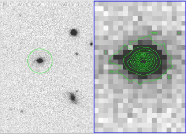
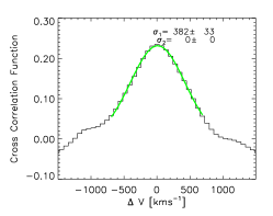
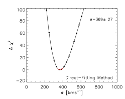
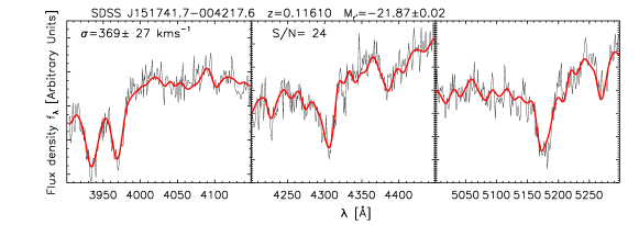
Figure 1.— Photometric and spectroscopic properties of objects with $\sigma>350$ km s^-1 and S/N$>10$ which are not obvious superpositions. Top left in each series of panels shows fields approximately $1\arcmin\times 1.5\arcmin$ and $7.6\arcsec\times 10.4\arcsec$ in size centred on the objects (each pixel is 0.4″ on a side). The SDSS spectrograph fibers are each 3″ in diameter, so neighbours more distant than this are unlikely to affect the observed spectrum. The top center panels show the cross-correlation between a template and the observed spectrum. Double-Gaussian fits to the cross correlation function, shown as two smooth red curves which sum to give the green curve, and yield estimates for the velocity dispersions of the individual components. The value of $\chi^{2}$ around its minimum, computed using a the direct-fit method assuming only a single broadening function, is shown in the top right panel of each series; text shows the estimated velocity dispersion. The bottom panels in each series show the result of using the direct-fit method to determine the pair of composite spectra which best-fit the observed spectrum; red solid lines show the combined spectrum of the best-fitting pair, the parameters of which are given in the left-most panel. For comparison, blue dotted lines show the best-fitting single component spectrum; text at the top of the panel shows the associated estimate of $\sigma$. In some cases the spectrum is best-fitted just by a single component; in these cases only a red solid line, showing the best-fitting single component, is presented. (The values of $\sigma$ reported in this Figure are not aperture corrected.)

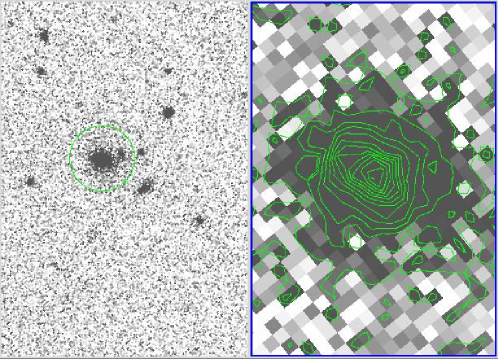
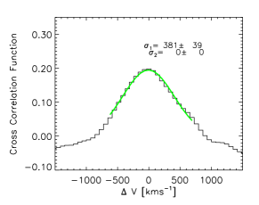
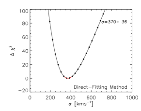
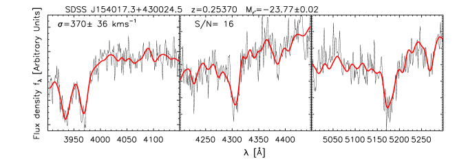
Figure 1.— Continued.

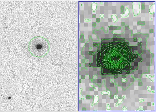
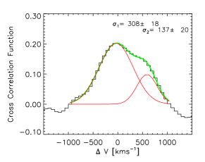
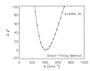
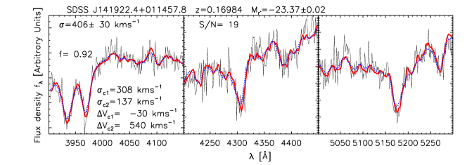
Figure 1.— Continued.

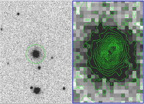
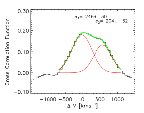
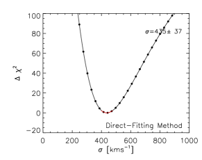
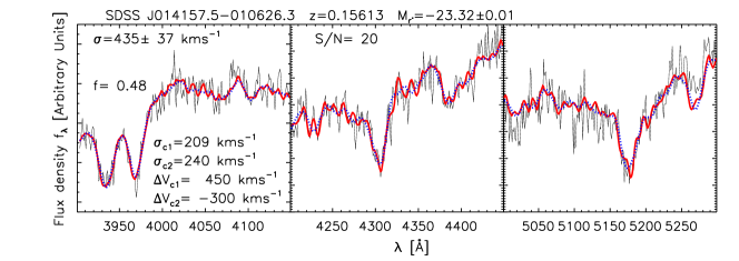
Figure 2.— As in Figure 1 but for objects classified as superpositions.

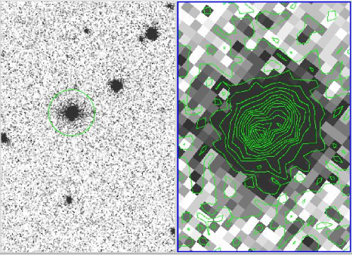
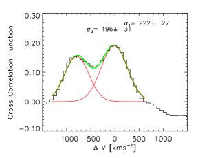
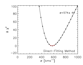
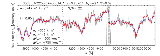
Figure 2.— Continued.

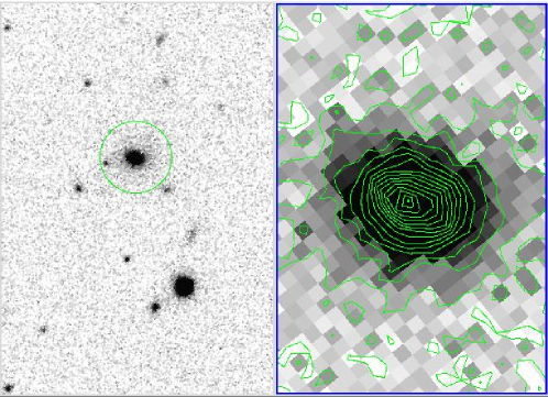
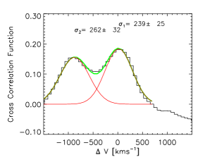
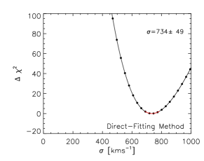
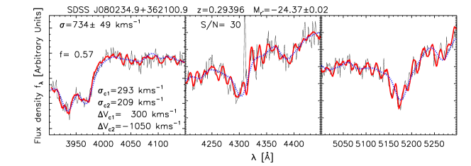
Figure 2.— Continued.

References

- (1) Abazajian, K., et al. 2003, AJ, 126, 2081
- (2) Bernardi, M., Sheth, R. K., Annis, J., et al. 2003a, AJ, 125, 1817
- (3) Bernardi, M., Sheth, R. K., Annis, J., et al. 2003b, AJ, 125, 1849
- (4) Bernardi, M., Sheth, R. K., Annis, J., et al. 2003c, AJ, 125, 1866
- (5) Bernardi, M., Sheth, R. K., Annis, J., et al. 2003d, AJ, 125, 1882
- (6) Bernardi, M., Sheth, R. K., Nichol, R. C. et al. 2005, AJ, 129, 61
- (7) Blanton, M.R., Lupton, R.H., Maley, F.M., Young, N., Zehavi, I., & Loveday, J. 2003, AJ, 125, 2276
- (8) Bruzual, G., & Charlot, S. 2003, MNRAS, 344, 1000
- (9) Budavari, T., Connolly, A. J., Szalay, A. S., et al. 2003, ApJ, 595, 59
- (10) Cohn, J. D., & Kochanek, C. S. 2004, ApJ, 608, 25
- (11) Dressler, A. 1979, ApJ, 231, 659
- (12) Eisenstein, D.J., et al 2001, AJ, 122, 2267
- (13) Ferrarese, L., & Merritt, D. 2000, ApJL, 539, L9
- (14) Franx, M., Illingworth, G. D., & Heckman, T. 1989, ApJ, 344, 613
- (15) Fukugita, M., Ichikawa, T., Gunn, J.E., Doi, M., Shimasaku, K., & Schneider, D.P. 1996, AJ, 111, 1748
- (16) Gebhardt, K., Bender, R., Bower, G., Dressler, A., et al., 2000, ApJ, 539, L13
- (17) Gunn, J.E., Carr, M.A., Rockosi, C.M., Sekiguchi, M., et al. 1998, AJ, 116, 3040
- (18) Hogg, D.W., Schlegel, D.J., Finkbeiner, D.P., & Gunn, J.E. 2001, AJ, 122, 2129
- (19) Jones, L. R., Ponman, T. J., Horton, A., Babul, A., Ebeling, H., & Burke, D. J., 2003, MNRAS, 343, 627
- (20) Jørgensen, I., Franx, M. & Kjærgaard, P. 1995, MNRAS, 276, 1341
- (21) Kravtsov, A. V., Berlind, A. A., Wechsler, R. H., Klypin, A. A., Gottloeber, S., Allgood, B., & Primack, J. R. 2004, ApJ, 609, 35
- (22) Lauer, T. R., Gebhardt, K., Richstone, D. et al. 2002, AJ, 124, 1975
- (23) Lupton, R., Gunn, J. E., Ivezić, Z., Knapp, G. R., Kent, S., & Yasuda, N. 2001, in ASP Conf. Ser. 238, Astronomical Data Analysis Software and Systems X, ed. F. R. Harnden, Jr., F. A. Primini, and H. E. Payne (San Francisco: Astr. Soc. Pac.), p. 269 (astro-ph/0101420)
- (24) Mitchell, J. L., Keeton, C. R., Frieman, J. A., & Sheth, R. K. 2004, ApJ, 622, 81
- (25) Miller, C. J., Nichol, R. C., Reichart, D. et al. 2004, AJ, in press
- (26) Navarro, J. F., Frenk, C. S., & White, S. D. M. 1997, ApJ, 490, 493
- (27) Pier, J.R., Munn, J.A., Hindsley, R.B., Hennessy, G.S., Kent, S.M., Lupton, R.H., & Ivezic, Z. 2003, AJ, 125, 1559
- (28) Porter, A. C., Schneider, D. P., & Hoessel, J. G. 1991, AJ, 101, 1561
- (29) Rix, H.-W., & White, S. D. M. 1992, MNRAS, 254, 389
- (30) Rusin, D., & Tegmark, M. 2001, ApJ, 553, 709
- (31) Sargent, W. L. W., Schechter, P. L., Boksenberg, A., Shortridge, K. 1977, ApJ, 212, 326
- (32) Scoccimarro, R., & Sheth, R. K. 2002, MNRAS, 329, 629
- (33) Sheth, R. K., Bernardi, M., Schechter, P. et al. 2003, ApJ, 594, 225
- (34) Simkin, S. M. 1974, A&A, 31,129
- (35) Smith, J.A., Tucker, D.L., Kent, S.M., et al. 2002, AJ, 123, 2121
- (36) Somerville, R. S., Moustakas, L. A., Mobasher, B., et al. 2004, ApJL, 600, 135
- (37) Stoughton, C., Lupton, R.H., Bernardi, M., et al. 2002, AJ, 123, 485
- (38) Strauss, M.A., Weinberg, D.H., Lupton, R.H. et al. 2002, AJ, 124, 1810
- (39) Tonry, J., & Davis, M. 1979, AJ, 84, 1511
- (40) Tremaine, S., Gebhardt, K., Bender, R., et al. 2002, ApJ, 574, 740
- (41) Vikhlinin, A., McNamara, B. R., Hornstrup, A., Quintana, H., Forman, W., Jones, C., & Way, M., 1999, ApJ, 520, L1
- (42) White, S. D. M., & Rees, M. J. 1978, MNRAS, 183, 341
- (43) White, S. D. M. & Frenk, C. 1991, ApJ, 379, 52
- (44) Worthey, G. & Ottaviani, D. L. 1997, ApJS, 111, 377
- (45) York, D.G., Adelman, J., Anderson, J.E., et al. 2000, AJ, 120, 1579
- (46) Yoshida, N., Sheth, R. K., & Diaferio, A. 2001, MNRAS, 328, 669
- (47) Zehavi I., et al., 2005, ApJ, 621, 22