Swift observations of the X-ray bright GRB 050315

Abstract

This paper discusses Swift observations of the $\gamma$-ray burst GRB 050315 (z=1.949) from $80$ s to $10$ days after the onset of the burst. The X-ray light curve displayed a steep early decay ($t^{-5}$) for $\sim 200$ s and several breaks. However, both the prompt hard X-ray/$\gamma$-ray emission (observed by the BAT) and the first $\sim 300$ s of X-ray emission (observed by the XRT) can be explained by exponential decays, with similar decay constants. Extrapolating the BAT light curve into the XRT band suggests the rapidly decaying, early X-ray emission was simply a continuation of the fading prompt emission; this strong similarity between the prompt $\gamma$-ray and early X-ray emission may be related to the simple temporal and spectral character of this X-ray rich GRB. The prompt (BAT) spectrum was a steep down to $\sim 15$ keV, and appeared to continue through the XRT bandpass, implying a low peak energy, inconsistent with the Amati relation. Following the initial steep decline the X-ray afterglow did not fade for $\sim 1.2\times 10^{4}$ s, after which time it decayed with a temporal index of $\alpha\approx 0.7$, followed by a second break at $\sim 2.5\times 10^{5}$ s to a slope of $\alpha\sim 2$. The apparent ‘plateau’ in the X-ray light curve, after the early rapid decay, makes this one of the most extreme examples of the steep-flat-steep X-ray light curves revealed by Swift. If the second afterglow break is identified with a jet break then the jet opening angle was $\theta_{0}\sim 5$^∘, and implying $E_{\gamma}\mathrel{\hbox{\hbox to0.0pt{\hbox{\lower 4.0pt\hbox{$\sim$}}\hss}\hbox{$>$}}}10^{50}$ erg.

1. Introduction

The Swift $\gamma$-ray burst Explorer (Gehrels et al. 2004) was successfully launched on 2004 November 20 and is now routinely taking observations of Gamma-ray Bursts (GRBs) and their afterglows in the crucial minutes to hours after the burst, delivering insights into the nature of the prompt emission and early afterglow phase. New bursts are detected by the Burst Alert Telescope (BAT; Barthelmy 2004; Barthelmy et al. 2005), a coded-mask imager with a with a $1.4$ sr field-of-view (half-coded) sensitive to $15-350$ keV energies, with imaging capability over the $15-150$ keV range. The spacecraft is able to slew autonomously to the burst position within a few tens of seconds. Once on-target, data are collected with two co-aligned narrow-field instruments: the X-ray Telescope (XRT; Burrows et al. 2004, 2005a) and the Ultraviolet/Optical Telescope (UVOT; Roming et al. 2005).

In this paper, we report on the Swift observations of GRB 050315. The BAT triggered and located on-board GRB 050315 at 2005-March-15 20:59:42 UT (Parsons et al. 2005). The spacecraft automatically slewed to the burst location, and the XRT and UVOT began observations starting $\approx 80$ s after the BAT trigger, one of the earliest XRT observations yet made. The XRT observation continued to detect the source for $\sim 10$ days, providing one of the best-sampled X-ray light curves of a GRB afterglow to date. At the time of writing there are $\sim 20$ Swift bursts with known redshifts, besides GRB 050315, four of these have XRT detections out $\sim 10$ day post-burst: GRB 050319 (Cusumano et al. 2005), GRB050525a (Blustin et al. 2005), GRB 050603 (Nousek et al. 2005) and GRB 050401 (De Pasquale et al. 2005). The spectroscopic redshift $z=1.949$ (Kelson and Berger 2005b) places GRB 050315 below the $z\approx 2.8$ mean redshift for Swift bursts estimated by Jakobsson et al. (2005).

In this paper we present a detailed analysis of the XRT data of GRB 050315 from the first minutes to several days after the burst. The plan for the paper is as follows. Section 2 reviews the basic details of the Swift observations from each instrument. Then section 3 presents a detailed analysis of the XRT images, light curve, and spectrum. Due to the very high initial count rate for the source, and the mode of the XRT camera during the observation, the early data suffered severely from pile-up, this problem is also discussed in section 3, along with a simple ‘workaround’ solution. Section 4 presents a comparison of the XRT and BAT data for the first few hundred seconds after the BAT trigger. Finally, section 5 summarises the main results and gives a brief discussion of some of the implications of this work. For the purpose of calculating luminosities the cosmological parameters were taken to be those of the WMAP standard cosmology, namely $H_{0}=70$ km s^-1 Mpc^-1 with $\Omega_{\rm m}=0.27,\Omega_{\Lambda}=0.73$.

2. Observations and basic data reduction

2.1. BAT observations

The BAT event data were analysed using the standard BAT analysis software (Build 20) as described in Swift BAT Ground Analysis Software Manual (Krimm, Parsons, & Markwardt 2004). Slew data were processed with the corrected ray-tracing procedure for slew data and light-curves and spectra extracted.

Figure 1 shows the BAT light curve which comprises two overlapping FRED-like peaks, and a possible precursor starting $\sim 60$ s before the trigger and continuing up to the main peak. The first peak rose over approximately $10$ s followed by a gradual decline, interrupted by a second peak at $T_{0}+$22 s. The burst duration including precursor was $T_{\rm 90}=96$ s. The BAT light curve from $T_{0}$ was binned such that each bin had a S:N greater than $3$ (i.e., $I/\sigma_{I}>3$) and was fitted with an exponential curve, $\exp(-t/t_{e})$. Ignoring the period $20-30$ s post-trigger, which was dominated by the second, shorter peak, the exponential curve gave a good fit ($\chi^{2}=35.39$ for $32$ degrees of freedom, dof, and a rejection probability of $p=0.69$) with a decay constant of $t_{e}=24\pm 2$ s. The hardness ratio time series, derived from four-band BAT light curves, clearly showed a softening of the burst spectrum with time.

The BAT spectra were extracted from the full time interval over which the burst was detected and also intervals covering the $1$ s peak, $T_{50}$ and $T_{90}$. The spectra were fitted over the $15-150$ keV range using XSPEC v11.3 (Arnaud 1996). In all cases a simple power law provided a good fit, with no evidence for a spectral break within the available bandpass; fitting with sharply breaking power law or a Band function (Band et al. 1993) did not substantially improve the fit ($\Delta\chi^{2}<4$). For the four time intervals the photon indices ($N_{\rm ph}(E)\propto E^{-\Gamma}$) were $\Gamma=2.16\pm 0.07$ (total), $2.3\pm 0.2$ ($1$ s peak), $2.02\pm 0.07$ ($T_{50}$) and $2.13\pm 0.07$ ($T_{90}$). The $1$ s peak flux was $2.2\pm 0.5$ ph cm^-2 s^-1 in the $15-150$ keV band (see also Sakomoto et al. 2005; Krimm et al. 2005) and the total burst fluence was $3.4\pm 0.3\times 10^{-6}$ erg cm^-2 (also $15-150$ keV).

If only a single photon index is measured it is difficult to constrain the bend or peak energy of a GRB spectrum. In order to constrain the bend energy for GRB 050315 a Band function was fitted to the BAT data from the full time interval assuming $\alpha=-1.3$ (the mean from the Amati et al. 2002 sample) but with all other parameters free. The bend energy $E_{0}$ was constrained to lie below $43$ keV (in the observed frame) at the $90$% confidence limit (CL). This corresponds to an upper limit on the peak energy $E_{\rm peak}=E_{0}(2-\alpha)$ of $30$ keV ($90$% CL) or $36$ keV ($99$% CL). Assuming $\alpha=-1.88$ (the steepest from the Amati et al. 2002 sample) gave an upper limit of $E_{\rm peak}<31$ keV ($90$% CL) or $40$ keV ($99$% CL), indicating the limit on $E_{\rm peak}$ is quite robust to the assumed value for $\alpha$.

Figure 1.— BAT light curve of GRB 050315 in $1$ s bins.

2.2. XRT observations

At the time of the BAT trigger the XRT was in Manual State, making pre-planned observations of GRB 050306 in Photon Counting (PC) mode, which meant that after the slew to GRB 050315 the standard set of XRT observations were not implemented and thus the early Image Mode (IM) snapshot, normally taken once the spacecraft has settled, was not taken in this instance. See Hill et al. (2004) and Burrows et al. (2004) for a description of the XRT readout modes. The absence of IM data immediately following the slew prevented an early XRT position determination. Ground analysis of the early PC data identified a new, rapidly fading source at (J2000) RA $=20^{\rm h}25^{\rm m}54^{\rm s}$, Dec $=-42\hbox{${}^{\circ}$}36\arcmin 0.2\arcsec$ (Morris et al. 2005).

There was also $0.9$ ks of exposure taken in Windowed Timing (WT) mode, during orbits when the XRT camera was rapidly switching between PC and WT modes due to high background. For most of these orbits there are not enough source counts for a robust detection and so these data were not used in the subsequent analysis.

The XRT data were processed by the Swift Data Center at NASA/Goddard Space Flight Center (GSFC) to level $1$ data products (calibrated, quality flagged event lists). These were further processed with the processing pipeline xrtpipeline v0.8.8 into level $2$ data products. The CCD operating temperature was between $-54.5$^∘C and $-61.5$^∘C, almost $50$^∘C warmer than the original design temperature, which led to a large number of hot and flickering pixels. These were flagged using the xrthotpix tool during the pipeline processing. High optical background light (e.g. due to the bright Earth limb) dominates XRT spectra at low energies, these events were filtered out in the pipeline processing and subsequently all events with energies $<0.2$ keV were ignored.

The first useful XRT data taken during the first orbit were $4$ frames ($10$ s) during the “settling” phase (when the pointing was within $10$ arcmin but not stable), starting at $T_{0}+73.5$ s. During the first CCD frame the source is spread over the image but it is relatively stable in the later three frames. These frames ($7.5$ s exposure from $76-83.5$ s post-burst) were included in the XRT data analysis. The pointed phase PC observation (once the spacecraft pointing was stable) began in earnest at $T_{0}+86$ s. Following this GRB 050315 was observed during a further $100$ orbits of Swift.

2.3. UVOT observations

In a $100$ s exposure taken approximately $90$ s after the trigger, UVOT detected no new source down to a $5\sigma$ limiting magnitude of $18.5$ in V-band (Rosen et al. 2005).

2.4. Other observations

Ground-based r-band observations with the LDSS instrument on Magellan/Clay detected a new source within the XRT error circle (Kelson and Berger 2005a). A $20$ min spectrum of the afterglow identified Al iii $\lambda\lambda 1854.7,~{}1862.8$ and Si ii $\lambda 1808.0$ absorption lines at a redshift $z=1.949$ (Kelson and Berger 2005b). Using the fluence of $3.4\times 10^{-6}$ erg cm^-2 this implies an isotropic equivalent $\gamma$-ray energy of $E_{\rm iso}=3.3\times 10^{52}$ erg (over $15-150$ keV in the observer frame).

Soderberg and Frail (2005) reported a VLA radio counterpart at 8.5 GHz at the location of the burst. Bersier et al. (2005) reported an I-band magnitude of $20.7$, $0.48$ days after the burst trigger. Cobb and Bailyn (2005), on behalf of the SMARTS consortium, found an R-band decay with a slope of $-0.57$ (over $11.6-35.6$ hr after the burst).

3. XRT analysis

3.1. Pile-up estimation

  

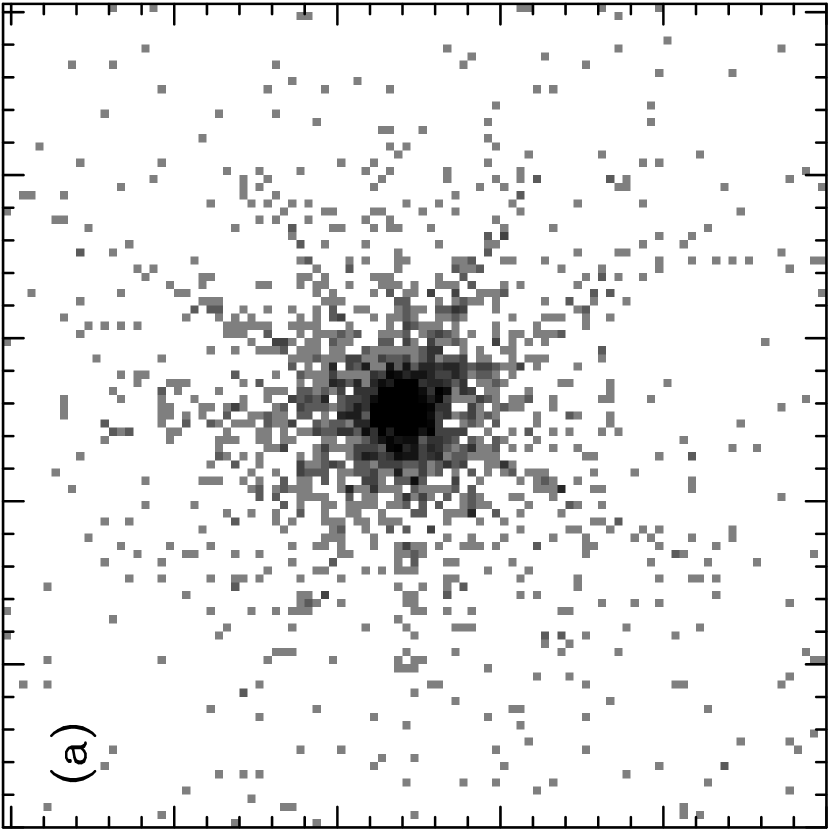
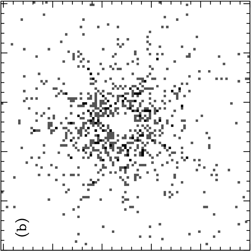
Figure 2.— XRT images of GRB 050315 in the $0.2-5$ keV range shown in detector coordinates. Panel (a) shows the events accumulated from the first $10$ orbits of pointed exposures, the image is $100$ pixels on a side (corresponding to $3.9$ arcmin). Panel (b) shows the image from only the first $60$ s of exposure, when the source was brighter than $>5$ ct s^-1, clearly showing a ‘hole’ in the centre of the image caused by pile-up.

If more than one X-ray photon is collected in a given detector pixel in a single frame, the charges produced by the two separate events are recorded as one. This effect is know as ‘pile-up.’ This is only part of the full story, however. The charge produced by a cosmic X-ray may be spread over one or more pixels (mono-pixel or split-pixel events), the shape of the charge distribution determines the ‘grade’ of the event (or ‘pattern’ in the XMM-Newton nomenclature). Pile-up also occurs when two X-rays are collected in neighbouring pixels in one frame (i.e. the patterns overlap). Such an event might be recorded as one split-pixel event rather than two separate events or it might be rejected entirely as diagonal charge patterns are not produced directly by X-rays. The effects of pile-up are an apparent loss of flux, particularly from the centre of the Point Spread Function (PSF), and a change in the grade distribution and energies of events at high input count rates.

Ballet (1999) presented a very thorough treatment of flux losses as a result of pile-up. Equation 6 of that paper shows how the observed rate of mono-pixel events varies with the true rate of incoming X-rays as a function of the CCD properties and the PSF. In order to examine at what count rates pile-up becomes significant for the XRT in PC mode this function was computed numerically, using different input count rates, assuming the following instrumental parameters. The clean (not piled-up) PSF was assumed to be a King profile (equation B1 of Ballet 1999) with parameters $r_{c}=6.49\arcsec$ and $\beta/2=1.59$, as measured for the XRT at $1.49$ keV from ground calibration tests (Moretti et al. 2004). The probability that an X-ray event produces a CCD event with a charge pattern containing $i$ pixels was $\alpha_{i}=\{0.778,~{}0.195,~{}0.014,~{}0.013\}$ for ($i=1,2,3,4$), as appropriate for the MOS CCD at $1.49$ keV.

The probability that an incident X-ray photon produces a mono-pixel event is thus $\alpha_{1}=0.778$ in the limit of no pile-up. See Ballet (1999) and Mukerjee et al. (2003) for more details. Using these numbers, and the CCD frame time of $\Delta T=2.507$ s, the rate of mono-pixel events, with and without pile-up, was computed as a function of input X-ray count rate. The results are shown in Table 1, where column $1$ shows the total input X-ray count rate ($\Lambda$), column $2$ shows the expected rate of mono-pixel events assuming no pile-up ($=\alpha_{1}\Lambda$), column $3$ shows the expected number of mono-pixel events after pile-up ($M_{1}$), and column $4$ shows the ratio of mono-pixel event count rates with and without pile-up ($\eta=M_{1}/\alpha_{1}\Lambda$). It was evident from this calculation that even at (observed mono-pixel event) count rates as low as $<0.1$ ct s^-1 the losses are $\sim 1$%, and by $1$ ct s^-1 the expected flux loss is $\sim 20$ per cent.

Table 1Effective losses due to pile-up.

Inputa	No pile-upb	Pile-upc	efficiencyd
(ct s-1)	(ct s-1)	(ct s-1)
$1.29\times 10^{-2}$	$1.00\times 10^{-2}$	$9.98\times 10^{-3}$	$0.998$
$1.29\times 10^{-1}$	$1.00\times 10^{-1}$	$9.78\times 10^{-2}$	$0.978$
$3.21\times 10^{-1}$	$2.50\times 10^{-1}$	$2.37\times 10^{-1}$	$0.947$
$6.43\times 10^{-1}$	$5.00\times 10^{-1}$	$4.49\times 10^{-1}$	$0.899$
$1.28$	$1.00$	$8.18\times 10^{-1}$	$0.818$
$3.21$	$2.50$	$1.63$	$0.652$
$6.43$	$5.00$	$2.53$	$0.507$
$1.29\times 10^{1}$	$1.00\times 10^{1}$	$3.81$	$0.380$
$3.21\times 10^{1}$	$2.50\times 10^{1}$	$6.37$	$0.255$
$1.29\times 10^{2}$	$1.00\times 10^{2}$	$1.30\times 10^{1}$	$0.131$

^a Rate of incoming X-rays: $\Lambda$

^b ‘True’ rate of mono-pixel events (excluding pile-up): $\alpha_{1}\Lambda$

^c ‘Observed’ rate of mono-pixel events (including pile-up): $M_{1}$

^d Ratio of observed/true count rates: $\eta=M_{1}/\alpha_{1}\Lambda$

3.2. Image Analysis

Figure 2 shows two images extracted from the first XRT dataset (observation ID $00111063000$, spanning the first $10$ orbits of data) and plotted in detector coordinates. Figure 2a shows the image formed from mono-pixel (grade = 0) events with photon energies in the range $0.2-5$ keV accumulated during the first $10$ orbits. There are virtually no source photons at energies $>5$ keV so only lower energy events were included in the analysis. Only single-pixel events were used as these should be affected least by pile-up. For comparison, Figure 2b shows the image formed from events in the same energy range, also from mono-pixel events, from only the first $60$ s of exposure, when the source was brighter than $>5$ ct s^-1. The centre of the second image is clearly deficient in counts due to pile-up.

Figure 3.— Radial profiles produced by integrating the counts in $2$-pixel wide annuli centred on the source centroid. The three profiles were extracted from times when the source was ‘bright’ ($>5$ ct s^-1), ‘intermediate’ ($1-5$ ct s^-1), and ‘faint’ ($<1$ ct s^-1). The data are shown with crosses, and the histogram shows the model (PSF $+$ background) that provided a good fit to the wings of the PSF (see text for discussion). Clearly when the source was faint the PSF model gave an accurate description of the radial profile, but when the source was brighter there was a substantial loss of counts at small radii.

The effects of pile-up were clearly illustrated by an examination of the X-ray image as a function of observed count rate. A preliminary light curve was accumulated from single-pixel, $0.2-5.0$ keV events extracted from a circle of radius $25$ pixels centred on the brightest pixel in the centre of the image shown in Figure 2a. The time bin size was set to be $25$ s (ten CCD frames). This light curve was used to define three time intervals: (i) ‘bright’ time, when the observed source count rate was $>5$ ct s^-1; (ii) ‘intermediate’ time, when the count rate was $1-5$ ct s^-1; and (iii) ‘faint’ time, when the count rate was below $<1$ ct s^-1. These three time intervals covered $60$ s, $113$ s and $12.15$ ks of exposure, respectively. For each time interval an X-ray image was formed, and a radial profile was calculated by binning the counts in $2$-pixel wide annuli centred on the source (taken to be at the centroid of the faint image).

The three radial profiles were compared to a model comprising an analytical PSF model and a constant background (per pixel) using XSPEC v11.3. Both the PSF and background models were integrated in annuli to compare with the measured radial profiles:

$$M(r_{in},r_{out})=\int_{r_{in}}^{r_{out}}\left[N\left\{1+\left(\frac{r}{r_{c}}\right)^{2}\right\}^{-\beta/2}+B\right]2\pi rdr$$ (1)

where the first term in square brackets represents the King profile PSF, with parameters $r_{c}$ and $\beta$, and the second term the constant background level, $B$. The PSF parameters were taken to be the same as used in section 3.4.

This model, with two free parameters (PSF normalisation, $N$, and background level, $B$) was fitted to the radial profile (counts per annulus), by adjusting the parameters to minimise the $C$-statistic (Cash 1979), which is equivalent to finding the maximum likelihood (ML) parameters from Poisson distributed data. The $C$-statistic was used as the fit statistic, instead of the more common $\chi^{2}$, because only the former gives the ML parameters when there are few counts per bin, as was the case here. The disadvantage of using the $C$-statistic is that is does not directly provide a goodness-of-fit measure, but this can be obtained through Monte Carlo simulations. For each model $10^{4}$ simulated profiles were generated, drawing each datum from the appropriate Poisson distribution, and the number of simulated data with a lower $C$-statistic (i.e. a better fit to the data) was used as a measure of the rejection probability $p$. The analytical PSF model provided a good fit to the faint radial profile, with $p=0.50$, confirming this model is indeed a good description of the source image at faint fluxes. The measured and fitted profiles are shown in Figure 3.

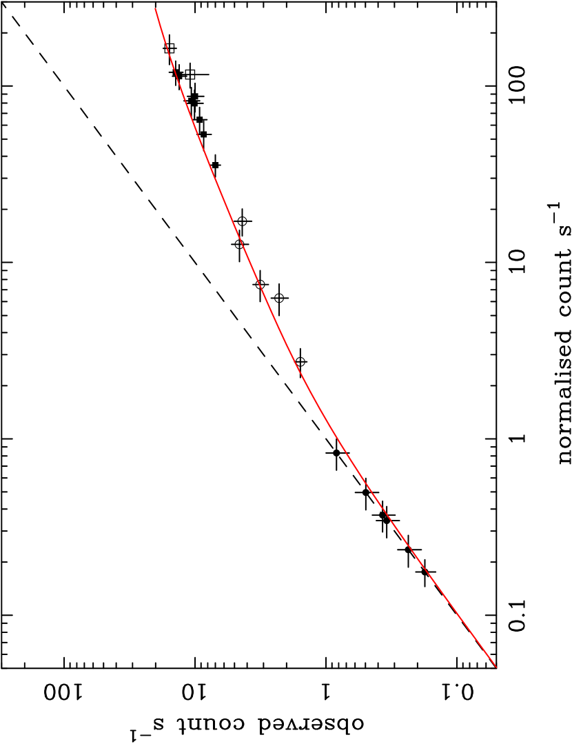
Figure 4.— Count rate losses due to pile-up. The abscissa represents the pile-up corrected count rate (i.e. after excluding the central part of the PSF and re-normalising to correct for the losses), which should be comparable to the true input source count rate. The ordinate represents the observed count rate extracted from a simple circular extraction region (i.e. without taking any account of pile-up). The hollow squares indicate the ‘settling’ data, the filled squares the ‘bright’ data, the hollow circles the ‘intermediate’ data and the filled circles the ‘faint data’ (the latter were not corrected for pile-up). The dashed curve marks the expectation in the limit of no pile-up. The solid curve marks the theoretically predicted relation between mono-pixel event count rates with and without pile-up effects, based on equation 6 of Ballet (1999).

The same model was then fitted to the radial profiles from the intermediate and bright images but gave an unacceptable fit to the data, with $p>0.9999$, in both cases, entirely due to the loss of counts in the centre of the image. Severe pile-up will produce a deficit of events in the central parts of the image, but the wings of the PSF should be relatively unaffected. Beyond some radius from the centre the observed image should be consistent with the PSF model; this radius was estimated by excluding the innermost annuli from the radial profiles until the fit became acceptable ($p<0.90$). In the case of the intermediate image ($1-5$ ct s^-1), excluding the innermost $8$ pixels radius ($19\arcsec$) gave a good fit ($p=0.797$), while for the bright image ($>5$ ct s^-1), the innermost $14$ pixels ($33.0\arcsec$) had to be excluded before the fit became acceptable ($p=0.863$).

As a final check for the effects due to pile-up at different fluxes, the data were divided into finer flux intervals. Radial profiles were extracted from times when the source was brighter than $10$ ct s^-1 and between $0.2-1.0$ ct s^-1. These were fitted with the PSF model as above. For the very brightest data, excluding the central $14$ pixels again provided an acceptable fit to the data ($p=0.635$), whereas excluding only the inner $12$ pixels did not ($p=0.969$). These results indicate that an inner radius cut-off of $14$ pixels (i.e. including only data from $\geq 15$ pixels away) is sufficient to exclude the piled-up region of the source image even at its brightest. Examining the image taken when the source count rate was $0.2-1.0$ ct s^-1, the PSF model gave a good fit down to the innermost pixel, confirming that pile-up is a weak effect at $\mathrel{\hbox{\hbox to0.0pt{\hbox{\lower 4.0pt\hbox{$\sim$}}\hss}\hbox{$<$}}}1$ ct s^-1 ($\mathrel{\hbox{\hbox to0.0pt{\hbox{\lower 4.0pt\hbox{$\sim$}}\hss}\hbox{$<$}}}20$% flux loss, see Table 1).

On the basis of the above analysis, the following ‘workaround’ procedure was used to mitigate the adverse effects of pile-up. Source events were extracted from a circular region of $60\arcsec$ ($25$ pixels) radius, excluding the centre of the region when the source was bright. In particular, for the period until $146$ s after the burst trigger, when the observed source count rate persistently exceeded $5$ ct s^-1, an annulus with inner and outer radii of $15$ and $25$ pixels was used for the extraction region. Data from the period from $146-259$ s, during which the source count rate was $1-5$ ct s^-1, were extracted between radii of $9$ and $25$ pixels. All data taken at later times, when the source flux was below $\sim 1$ ct s^-1 were extracted using a full circular region. Data extracted from annular regions were renormalised to account for the loss of the central part of the PSF. The correction factors, calculated by integrating the King PSF model, were $14.4$ and $5.0$ for the data extracted during bright, intermediate fluxes, respectively.

Figure 5.— Light curve of GRB 050315 in the $0.2-5$ keV band. These data have been corrected for pile-up; the different symbols reflect the different corrections. The symbols have the same meaning as in Fig. 4. Times are in the observed frame (i.e. not corrected for cosmological time dilation).

The overall effect of pile-up can be seen by comparing the light curve extracted from the first orbit of data before and after pile-up correction. Figure 4 shows the relationship between the corrected and uncorrected count rates, which indicates the effect of pile-up as a function of source intensity. Also shown is the theoretical curve derived from equation 6 of Ballet (1999), and discussed in section 3.1, for the relation between mono-pixel event count rates with and without pile-up effects. Clearly the empirical correction of pile-up matches the theoretical expectation based on the known CCD and PSF characteristics.

3.3. Timing Analysis

The $0.2-5$ keV light curve of GRB 050315 was extracted from the full XRT dataset. The first orbit, when the source was at its brightest, was treated separately to avoid pile-up. The data were extracted in $2.507$ s bins (i.e. one CCD frame) and then rebinned such that each time bin contained $\geq 25$ events. (This permits the use of $\chi^{2}$ minimisation as a ML method.) Error bars were calculated using counting statistics. The three different time intervals during which the source was ‘bright,’ ‘intermediate’ and ‘faint’ were extracted using the different regions, to account for different degrees of pile-up, as discussed above. A background light curve was extracted, from an annulus centred on the source with inner and outer radii of $60$ and $120$ pixels ($141-283\arcsec$), respectively, and subtracted from the source light curve. The three light curves from the different brightness intervals were renormalised to account for PSF losses; the resulting pile-up corrected light curve is shown in Figure 5. Also included in this figure are the data taken from the settling phase (see section 2.2), treated for pile-up in the same fashion as the ‘bright’ data.

The other orbits, for which pile-up is not an issue, were extracted in the standard fashion, using a $60\arcsec$ circular source region and the same background region as for the first orbit. These data were binned to produce one bin per orbit, accepting only those orbits containing at least $15$ counts within the source region. The light curve spanning all XRT observations of GRB 050315 is shown in Figure 5.

Table 2Results of XRT light curve fitting.

Orbits	$\alpha$	$t_{\rm br}$ (s)	$\alpha$	$t_{\rm br}$ (s)	$\alpha$
$1$	$1.8\pm 0.9$	$115\pm 12$	$5.2_{-0.4}^{+0.5}$	$308_{-33}^{+38}$	$1.2\pm 0.6$
$2+$	$<0.41$	$1.2_{-0.3}^{+0.5}\times 10^{4}$	$0.71\pm 0.04$	$2.5_{-0.3}^{+1.1}\times 10^{5}$	$2.0_{-0.3}^{+1.7}$
All	$1.9_{-1.0}^{+0.7}$	$118\pm 12$	$5.3_{-0.4}^{+0.5}$
	$0.06_{-0.13}^{+0.08}$	$1.2\pm 0.4\times 10^{4}$	$0.71\pm 0.04$	$2.5_{-0.3}^{+1.1}\times 10^{5}$	$2.0_{-0.3}^{+1.7}$

NOTE: The models fitted to the first orbit ($76-778$ s post burst) and later orbits ($5\times 10^{3}-9\times 10^{5}$ s) were doubly broken power laws, with slopes and break times as stated. The model fitted to all data was the sum of a singly broken power law and a doubly broken power law.

The light curve was parameterised by fitting simple analytical models, comprising connected power laws [e.g. $F(t)\propto(t-T_{0})^{-\alpha}$], using XSPEC to minimise the $\chi^{2}$ fit statistic. Initially, the first orbit ($76-778$ s post burst) and later orbits ($5\times 10^{3}-9\times 10^{5}$ s) were treated separately, before fitting the entire light curve. Through this section, and the rest of the paper, uncertainties on fitted parameters correspond to $\Delta\chi^{2}=2.706$ (i.e. a nominal $90$% confidence region), unless stated otherwise.

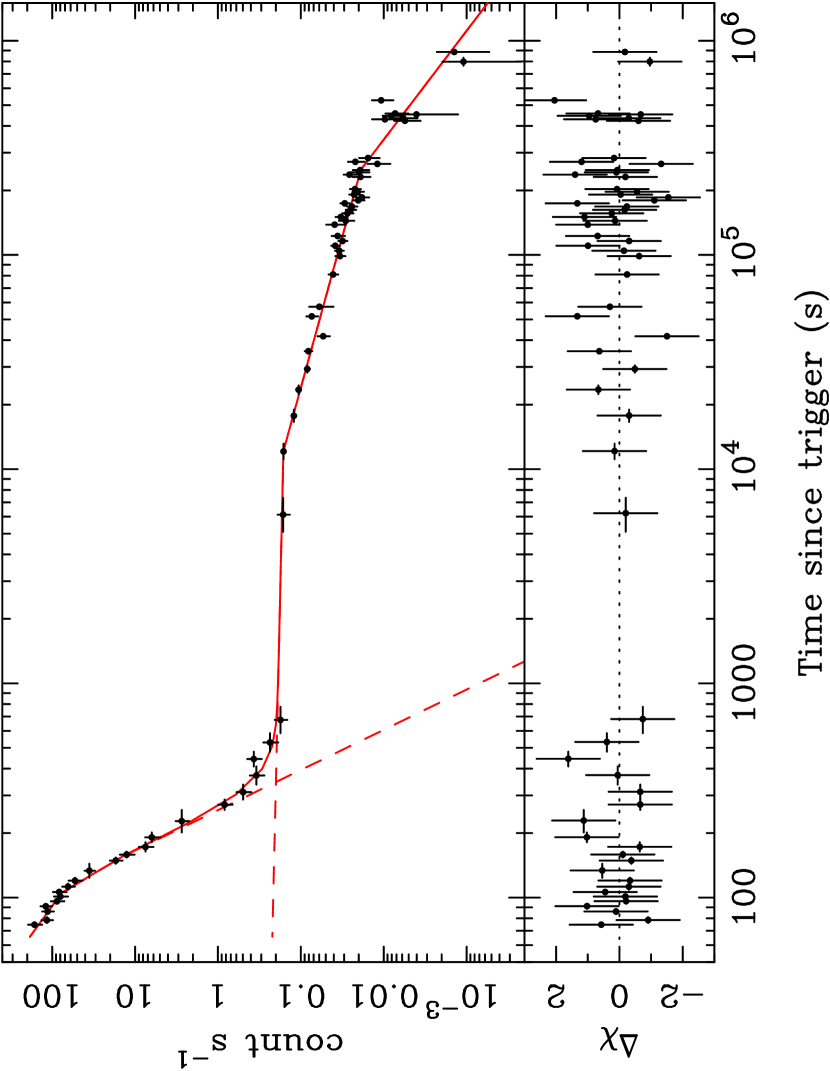
Figure 6.— Light curve of GRB 050315 in the $0.2-5$ keV band, as in Fig. 5, also showing the best-fitting model comprising a singly broken power law and a double broken power law, which dominate at early and late times, respectively (see Table 2). The lower panel shows the $(data-model)/\sigma$ residuals.

A power law with no breaks or just one break did not fit the first orbit data (rejection probability $p>0.9999$), whereas a doubly broken power law gave a very good fit ($\chi^{2}=6.90$ with $15$ dof and $p=0.04$). (Even after discounting the $2$ time bins from the ‘settling’ data the improvement between singly-broken and doubly-broken power law is significant at $99.4$% confidence using an $F$-test.) The light curve for the first $700$ s is strongly curved on a $\log[F_{\rm X}]-\log[t-T_{0}]$ plot (Figure 5), progressing through flat then steep then flat phases. The best-fitting parameters for the doubly-broken power law model are given in the first row of Table 2. The initial steepening of the decay during the first $\approx 200$ s is reminiscent of an exponential decay, as observed in the prompt BAT light curve (section 2.1). This possibility is discussed further below.

The later orbit light curve was also inconsistent with a power law ($p>0.9999$) but a singly broken power law provided a good fit ($\chi^{2}=38.86$ with $39$ dof and $p=0.52$). However, including a second break improved the fit substantially ($\chi^{2}=28.63$ with $37$ dof and $p=0.16$). This improvement is significant at $99.6$% confidence, using the $F$-test. A smooth bend from one power law index to another gave a much worse fit that two sharp breaks. The late-time data therefore also show two break times (as given in the second row of Table 2). Thus the complete XRT light curve for GRB 050315 shows at least 4 breaks if interpreted as a series of connected power laws. In fact, the complete light curve is well fitted by the sum of two components, a singly broken power law dominating before $\sim T_{0}+300$ s and a doubly broken power law dominating afterwards ($\chi^{2}=38.77$ for $54$ dof; $p=0.06$). The best-fitting parameters for this model are shown in Table 2 (rows $3$ and $4$) and the model is shown in Figure 6.

The only way to reconcile the early (flat-steep) part of the light curve with a single (unbroken) power law is by allowing the start time to be $165\pm 11$ s prior to the BAT trigger, which lies well before the precursor in the BAT light curve (see Figure 1), in which case the early decay slope is $\alpha=8.9_{-1.5}^{+0.1}$. This model gave an acceptable fit but not as good as the the model with a break at $T_{0}+120$ s ($\chi^{2}=54.46$ for $55$ dof; $p=0.47$).

Fitting the steep, early light curve with an exponential decay (plus the doubly broken power law component to fit the later time data) also gave a good fit, with $t_{e}=35\pm 2$ s, although not as good as the broken power law ($\chi^{2}=47.76$ for $56$ dof, $p=0.23$). Extrapolating the exponential (prompt) plus broken power law (afterglow) model between $10^{-2}-10^{7}$ s the total luminosity in the late-time broken power law component is $\sim 32$% of that in the ‘prompt’ exponentially decaying component (assuming no spectral evolution).

3.4. Spectral Analysis

XRT spectra were extracted from mono-pixel events collected from source and background regions and grouped such that the source spectrum contained at least $20$ counts per bin. (Fitting the raw, un-grouped data using the $C$-statistic did not alter the main results.) Five spectra were extracted from the following time intervals. From the first pointing there were three intervals: ‘bright,’ ‘intermediate’ and ‘faint’ as discussed above. One spectrum was extracted from the second pointing, which lasted from $0.69-2.4\times 10^{5}$ s post-burst (with an exposure time of $40.5$ ks). This is referred to as the ‘mid’ spectrum and lies on the $\alpha\approx 0.7$ part of the decay light curve. The fifth spectrum was extracted from the fourth pointing, which lasted from $2.7-5.3\times 10^{5}$ s post-burst (with an exposure time of $18.7$ ks). This is referred to as the ‘late’ spectrum and lies on the $\alpha\approx 2.0$ part of the decay light curve. (The third, fifth and later pointings only provided $<100$ source counts and so were not used in the spectral analysis). The data were corrected for pile-up by extracting source counts from annuli with radii $15-25$ and $9-25$ (inclusive) pixels during the ‘bright’ and ‘intermediate’ time intervals, as for the light curve, and using an appropriate ancillary response file to correct for the PSF losses.

Figure 7.— XRT spectra of GRB 050315. From the top down these correspond to the following time intervals: $86-146$ s (‘bright’), $146-259$ s (‘intermediate’), $259$ s to $57.39$ ks (‘faint’), $0.69-2.4\times 10^{5}$ s (‘mid’) and $2.7-5.3\times 10^{5}$ s (‘late’). The data are shown with crosses and the best-fitting absorbed power law model in each case (see Table 3) is shown as a histogram

These spectra were fitted with absorbed power law models. The Galactic column in the direction of GRB 050315 is $N_{\rm H}=4.3\times 10^{20}$ cm^-2 (Dickey & Lockman 1990), and this was kept fixed, using the TBabs model of Wilms, Allen & McCray (2001). A second neutral absorber in the GRB frame (i.e. $z=1.949$) was included to model any intrinsic absorption. The five XRT spectra are shown in Figure 7. In all cases a power law with excess absorption provided a good fit to the data. The results for the XRT spectral fitting are shown in Table 3, along with the results of fitting the BAT spectra. There is evidence that the spectrum softened between the ‘bright’ spectrum (i.e. $<T_{0}+146$ s) and the ‘faint’ spectra (i.e. $>T_{0}+259$ s), but the absorption columns remain consistent within the errors. This is illustrated by Figure 8 which shows the $\Delta\chi^{2}$ contours for the slope and column derived from the ‘bright’ and ‘faint’ data.

Table 3Results of BAT and XRT spectral fitting.

Data	Time ($+T_{0}$ s)	$\Gamma$	$N_{\rm H}$	$\chi^{2}$	dof	$p$
BAT peak	$25.6-26.6$	$2.3\pm 0.2$		$51.79$	$56$	$0.37$
BAT $T_{50}$	$0.0-24.7$	$2.02\pm 0.07$		$56.11$	$56$	$0.53$
BAT $T_{90}$	$-48-48$	$2.13\pm 0.07$		$51.43$	$56$	$0.35$
BAT total	$-56-69$	$2.16\pm 0.07$		$55.34$	$56$	$0.50$
XRT bright	$76-146$	$2.5\pm 0.4$	$1.2\pm 0.7$	$21.01$	$14$	$0.90$
XRT inter	$146-259$	$2.9_{-0.8}^{+1.0}$	$<2.1$	$2.07$	$5$	$0.16$
XRT faint	$259-5.7\times 10^{4}$	$1.73\pm 0.11$	$0.5\pm 0.2$	$57.76$	$51$	$0.76$
XRT mid	$0.69-2.4\times 10^{5}$	$1.79\pm 0.13$	$0.8\pm 0.3$	$48.98$	$50$	$0.49$
XRT late	$2.7-5.3\times 10^{5}$	$1.7_{-0.3}^{+0.5}$	$<1.0$	$5.0$	$8$	$0.24$
BAT+XRT		$2.18\pm 0.07$	$0.6\pm 0.4$	$79.65$	$71$	$0.76$

NOTE: $N_{\rm H}$ is in units of $10^{22}$ cm^-2 at $z=1.949$.

Figure 8.— Confidence contours for spectral model parameters (excess absorption column and photon index) as fitted to the ‘bright’ ($86-146$ s) and ‘faint’ ($259$ s to $57.39$ ks) XRT data. The lines shown are the $\Delta\chi^{2}=2.30$, $4.61$ and $9.21$ contours (nominal $68.3$, $90$ and $99$% confidence bounds). The photon index clearly decreased between ‘bright’ and ‘faint’ spectra. (The contours for the ‘mid’ and ‘later’ data are not shown but do overlap with those for the ‘faint’ data.)

4. BAT-XRT comparison

The early (‘bright’) XRT spectrum (section 3.4) showed a power law slope not dissimilar to that of the BAT spectrum (section 2.1). As a test of whether the early X-ray emission was connected to the prompt $\gamma$-ray emission, the BAT and early XRT spectra were fitted simultaneously. Figure 9 shows the XRT spectrum from the ‘bright’ data ($\approx 86-146$ s post-trigger) and the BAT spectrum (extracted from the full time interval) fitted with the same absorbed power law model, but with different normalisations between the two spectra (which allows for the temporal decay between the times of the BAT and early XRT observations). A single absorbed power law gave a good fit to the combined data (see Table 3), consistent with the hypothesis that the early X-ray emission and prompt hard X-ray/$\gamma$-ray emission were produced by the same emission spectrum.

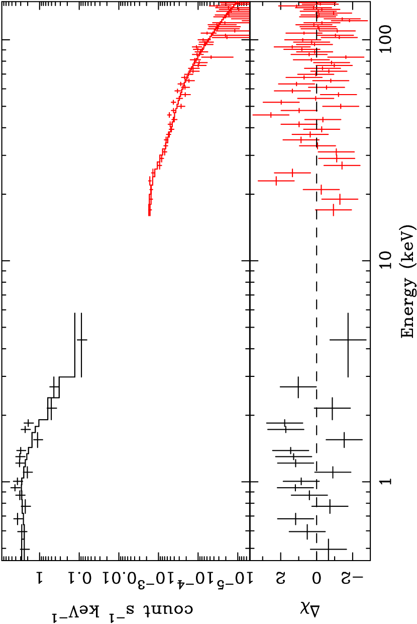
Figure 9.— Spectra from the BAT (on the right) from $T_{0}-56$ s to $T_{0}+69$ s and ‘bright’ XRT data (on the left) from $T_{0}+76$ s to $T_{0}+146$ s, fitted simultaneously with a single absorbed power law ($\Gamma=2.15\pm 0.07$).

The spectral fits to the BAT and XRT data were used to calculate the conversion between observed count rate and unabsorbed $0.2-10.0$ keV flux for both BAT and XRT. The extrapolation of the BAT spectrum into the XRT bandpass should be reasonably accurate since, as shown above, the prompt spectrum does extend, unbroken, into the XRT bandpass. These factors were then used to plot the XRT and BAT light curves in flux units, for comparison with one another. The error on the BAT flux resulting from the uncertainty in the spectral model was propagated into the $0.2-10.0$ keV band and added in quadrature with the statistical error. The result is shown in Figure 10. From this figure it is clear that the tail end of the prompt emission seen by the BAT lies very close to the early XRT data, strongly supporting the idea that the early X-ray emission is an extension of the fading prompt emission. The combined BAT-XRT light curve is dominated by an approximately exponential decay in flux. (The agreement between BAT and XRT light curves does not depend on whether absorbed or unabsorbed fluxes are plotted.)

5. Discussion

5.1. Summary of results

The following are the main results of the XRT and BAT temporal and spectral analyses of the Swift observations of GRB 050315.

• The BAT light curve showed two FRED-like peaks. The main peak fell away exponentially with a decay constant of $\approx 24\pm 2$ s in the observer’s frame ($t_{e}=8\pm 1$ s in the source frame). See Figure 1.

• After correcting for pile-up, the XRT light curve starting at $T_{0}+76$ s showed a very rapid decline (as steep as $\alpha\mathrel{\hbox{\hbox to0.0pt{\hbox{\lower 4.0pt\hbox{$\sim$}}\hss}\hbox{$>$}}}5$) until $\approx T_{0}+300$ s. The e-folding time during this period was $35\pm 2$ s in the observer’s frame ($12\pm 1$ s in the source frame). See Figures 5 and 6.

• Despite modest spectral evolution in the BAT data, the BAT and early ($\mathrel{\hbox{\hbox to0.0pt{\hbox{\lower 4.0pt\hbox{$\sim$}}\hss}\hbox{$<$}}}T_{0}+150$ s) XRT spectra were both consistent with steep power laws ($\Gamma\approx 2.2$). See Figure 9.

• Extrapolating the BAT light curve into the XRT energy band (using the best-fitting XRT+BAT spectral model) showed the early X-ray data to be consistent with the tail end of the exponentially decaying prompt emission. See Figure 10.

• The XRT spectra show significant excess absorption in the rest frame of GRB 050315 ($N_{\rm H}\sim 10^{22}$ cm^-2) with significant spectral hardening between early ($\mathrel{\hbox{\hbox to0.0pt{\hbox{\lower 4.0pt\hbox{$\sim$}}\hss}\hbox{$<$}}}T_{0}+150$ s) and later ($\mathrel{\hbox{\hbox to0.0pt{\hbox{\lower 4.0pt\hbox{$\sim$}}\hss}\hbox{$>$}}}T_{0}+250$ s) times. See Figures 7 and 8.

• After $T_{0}+300$ s the X-ray flux decays only very slowly but shows further temporal breaks at $1.2\pm 0.4\times 10^{4}$ s ($4.1\pm 1\times 10^{3}$ s source frame) to a slope of $\alpha\approx 0.7$, and again at $2.5_{-0.3}^{+1.1}\times 10^{5}$ s ( $8_{-1}^{+3}\times 10^{4}$ s source frame) to a steeper slope of $2.0_{-0.3}^{+1.7}$. See Figures 5 and 6.

5.2. Prompt hard X-ray/$\gamma$-rays from GRB 050315

GRB 050315 shows a relatively soft (steep) spectrum in both the BAT and early XRT data ($\Gamma\approx 2.2$). This has at least two interesting implications. The first is that GRB 050315 may be classified as an ‘X-ray rich’ GRB or an ‘X-ray flash’ (XRF). These classifications are often made using the softness ratio $SR=\log[S_{\rm X}(2-30~{}{\rm keV})/S_{\gamma}(30-400~{}{\rm keV})]$ (Lamb et al. 2004; Sakamoto et al. 2004), with $-0.5<SR<0$ for an X-ray rich burst and $SR>0$ for an XRF. The joint BAT-XRT spectral fit (section 4) gave $SR=0.2$, suggesting that GRB 050315 may be better classified as an XRF.

The second implication of the soft spectrum is that the energy at which the emission peaks (the peak in $EF_{E}$ space) is below the observed BAT energy range. This does not match the expectations of the $E_{\rm iso}-E_{\rm peak}$ relation discovered by Amati et al. (2002). These authors showed that the peak energy and isotropic energy were correlated for a small sample of GRBs with known redshifts detected by BeppoSAX. Ghirlanda, Ghisellini & Firmani (2005) found the same relation in BATSE data. Using the $E_{\rm peak}-E_{\rm iso}$ relation from Ghirlanda et al. (2005; their equation 1) the predicted peak energy for GRB 050315 is $E_{\rm peak}\sim 163$ keV in the source frame, or $\sim 55$ keV in the observed frame, yet the observed BAT spectrum was an unbroken power law with $\Gamma\approx 2.2$ down to $\sim 15$ keV, suggesting a much lower $E_{\rm peak}$. As shown in section 2.1 the peak energy (in the observer’s frame) was constrained to $E_{\rm peak}\mathrel{\hbox{\hbox to0.0pt{\hbox{\lower 4.0pt\hbox{$\sim$}}\hss}\hbox{$<$}}}30$ keV ($90$% CL) which is at odds with the prediction of the Amati relation. Furthermore, the estimated $E_{\rm iso}$ is really a lower limit since it was calculated over only $15-150$ keV, meaning the predicted $E_{\rm peak}$ is a lower limit. If the true $E_{\rm iso}$ is higher, the predicted $E_{\rm peak}$ is also higher and discrepancy with the Amati relation becomes even more severe.

5.3. Prompt-afterglow transition in X-rays

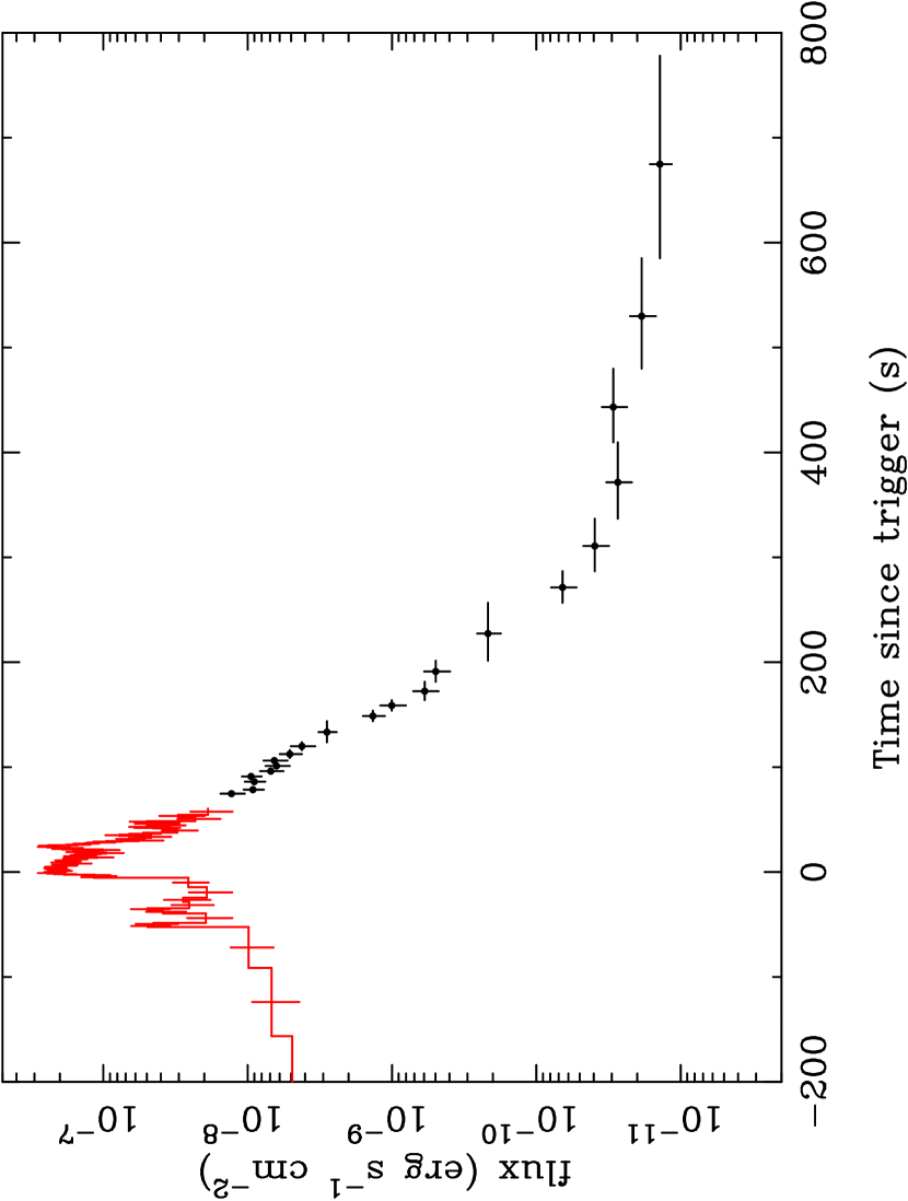
Figure 10.— Light curves from the BAT (histogram) and first orbit of XRT data (crosses) plotted in units of (unabsorbed) flux in the $0.2-10.0$ keV band. The hard X-ray BAT light curve was extrapolated into the XRT energy band using the spectral fit discussed in section 4.

The similarity of the spectral slopes from the early XRT data and the prompt BAT observation (Figure 9) raises the interesting possibility that the prompt hard X-rays and early soft X-rays do not come from distinct components (‘burst’ and ‘afterglow’) but are actually different parts of the same spectrum. The early soft X-rays may simply be the lower energy emission from the same component as the prompt hard X-ray/$\gamma$-ray emission that triggered the BAT. That the predicted soft X-ray flux from the BAT data matches the observed flux at the start of the XRT observation (Figure 10) strongly supports this idea; furthermore, both the prompt hard X-rays and early soft X-rays decay in an approximately exponentially fashion with similar e-folding timescales. Small differences in fluxes and decay timescales between the two bands are perhaps not surprising given that the spectrum of the prompt emission does evolve slightly (gets softer) with time. For example, if the X-ray flux is given by $F(t)\propto E^{-\beta(t)}\exp(-t/t_{e})$, where $\beta=\Gamma-1$, and $\beta(t)$ increases slightly with time, the softer X-rays would decay slightly slower, as observed.

If the X-ray emission before $\sim T_{0}+300$ s ($100$ s in the source frame) is dominated by the decay of the prompt burst spectrum, the subsequent emission may be identified with the more standard X-ray afterglow (Costa et al. 1997) which must have begun as the prompt emission decayed. The change in the X-ray spectrum after $\sim T_{0}+300$ s (see Figure 8) supports the idea that these two time intervals should be considered as distinct phases. In the following discussion the emission before and after $\sim T_{0}+300$ s will be referred to as ‘prompt’ and ‘afterglow,’ respectively. In the standard relativistic fireball models (e.g. van Paradijs, Kouveliotou & Wijers 2000; Mészáros 2002; Piran 2005) the prompt emission is caused by internal shocks within the expanding fireball, and the afterglow is the result of the external shocks, as the relativistic matter collides with circum-burst material. The X-ray to $\gamma$-ray emission observed before $T_{0}+300$ s, with a spectral slope $\Gamma\approx 2.2$, is therefore identified with internal shocks and the emission observed afterwards, with a spectral slope $\Gamma\approx 1.8$, is identified with the external shocks.

Some other Swift bursts do not show such a strong connection between the BAT and XRT data, e.g. GRB 050219a (Tagliaferri et al. 2005). But the results for GRB 050315 are not completely without precedent. Tagliaferri et al. (2005) also reported the Swift observations of GRB 050126, with a simple FRED-like burst profile. When extrapolated into the XRT energy range, the predicted flux at the end of the BAT light curve is of the same order as the observed flux in the early (from $\sim T_{0}+100$ s) XRT light curve. However, in this case, the prompt BAT spectrum was considerably harder than the early XRT spectrum. More convincing was GRB 050319 (Cusumano et al. 2005; Barthelmy et al. 2005) for which the spectra from the prompt BAT and early XRT data were consistent, and the X-ray light curve was consistent with a single rapid decay from prompt emission, until overtaken by a more slowly fading X-ray afterglow at $\sim T_{0}+400$ s, which showed a harder X-ray spectrum. GRB 050117 (Hill et al. 2005) also showed reasonable agreement between the predicted X-ray flux from the BAT and the earliest X-ray flux measured by the XRT, despite the complex burst profile.

Several other Swift XRT observations of GRBs have revealed very rapid X-ray decays in the first few hundred s after the bursts (Hill et al. 2005; Tagliaferri et al. 2005). These may also be caused by the fading prompt source, perhaps off-axis emission (Kumar & Panaitescu 2000), in which case the mis-matches between BAT and XRT light curves require explanation. It is conceivable this is due to dramatic spectral evolution. After the first few $10^{2}$ s the X-ray emission is dominated by the afterglow which stayed relatively constant before decaying as a broken power law.

5.4. The X-ray ‘plateau’ phase

From $\approx 300$ s until $\approx 1.2\times 10^{4}$ s ($100-4\times 10^{3}$ s in the source frame) the X-ray afterglow emission was almost perfectly constant ($\alpha_{0}=0.06_{-0.13}^{+0.08}$; using the convention that $F(\nu,t)\propto t^{-\alpha}\nu^{-\beta}$, where $\beta=\Gamma-1$), beyond which it broke to a power law decay with a slope of $\alpha_{1}=0.7$. Such a flat afterglow light curve is unusual and has not been seen in other Swift bursts to date although several other bursts have shown less extreme steep-flat-steep light curves (e.g. Chincarini et al. 2005; Hill et al. 2005). It must be said however that the sampling during this period is rather sparse and it remains possible, though perhaps unlikely, that an X-ray re-brightening episode, such as observed in GRB 050406 and GRB 050502b (Burrows et al. 2005b), could have occurred during the gaps in the light curve, masking an underlying shallow decay.

The indices of the temporal decay and energy spectrum of the afterglow, $\alpha$ and $\beta$, respectively are governed by the power law index of the energy distribution of the electrons in the flow, $p$. The X-ray spectrum during the plateau phase (‘faint’ and ‘mid’ spectra; Table 3) shows an energy index of $\beta\sim 0.7$. This rules out the X-ray band lying on the $\beta=-1/3$ part of the synchrotron spectrum, below the emission frequency of lowest Lorentz factor electrons in the shock, $\nu_{m}$, and the synchrotron cooling frequency, $\nu_{c}$ (e.g. Sari, Piran & Narayan 1998). However, this spectral index is close to the $\beta\sim 0.5$ expected if the X-ray band lies above $\nu_{c}$ but below $\nu_{m}$. In this case the flux is expected to decay with $\alpha=1/4$, which is steeper than the observed platau phase ($\alpha\approx 0$), but a flatter decay could occur if inverse-Compton scattering makes a significant contribution to electron cooling, this might be expected for the first few hours of a typical burst. After $\nu_{m}$ moves below the X-ray band (which occurs as $\nu_{m}\propto t^{-3/2}$), the expected decay steepens to $\alpha=(3p-2)/4$, thus a slope of $\alpha\approx 0.7$ predicts $p\approx 1.6$. Such a low $p$ value is unusual, but not totally without precedent (e.g., GRB 010222; Masetti et al. 2001). Thus the break from $\alpha\approx 0$ to $0.7$, marking the end of the plateau phase, could be due to $\nu_{m}$ moving below the X-ray band (in the standard forward shock model it is difficult to have $\nu_{m}$ much above the XRT band after $300$ s).

Alternatively the plateau phase of the light curve may be a consequence of ‘refreshed’ shocks, i.e. energy is pumped into the shock as it occurs. There are two simple scenarios that will result in refreshed shocks. The first is that there is a distribution of Lorentz factors in the jet such that slower material is continuously catching-up with faster ejecta as it decelerates in the shock (e.g. Rees & Mészáros 1998; Sari & Mészáros 2000). The second scenario occurs when the central engine stays active for a prolonged period, and continuously injects energy into the jet at a decreasing rate (e.g. Zhang & Mészáros 2001). After the energy injection ends (at $\sim 12$ ks) the flux would be expected to decay as a power law with an index $\alpha=3(p-1)/4$ provided that $\nu_{c}$ was above the XRT band. Using $p=1+2\beta\approx 2.4$ gives $\alpha\approx 1.1$ for a uniform density ISM, and steeper still for a medium consisting of the progenitor wind, inconsistent with the observations ($\alpha\approx 0.7$). If, on the other hand, $\nu_{c}$ was below the XRT band then $p=2\beta\approx 1.4$ and the flux decline is given by $\alpha=-(3p-2)/4=0.55$ which is closer to the observed decline. This solution also requires $p<2$.

5.5. Late-time X-ray break

The X-ray afterglow shows a second break at $2.5\times 10^{5}$ s ($8.4\times 10^{4}$ s in the source frame) to a much steeper decline, with $\alpha_{2}=2.0_{-0.3}^{+1.7}$. This might readily be identified with a ‘jet break,’ corresponding to the time when the beaming angle of the relativistic flow ($\theta_{\rm beam}\sim\gamma^{-1}$) becomes wider than its geometrical opening angle ($\theta_{0}$), after which the emission decays much faster (Sari, Piran & Halpern 1999; Rhoads 1999). Using equation 1 of Frail et al. (2001) the observed break timescale and $E_{\rm iso}$, yield a jet opening angle of $\theta_{0}\sim 5$^∘, similar to the values derived for other bursts (Frail et al. 2001; Ghirlanda et al. 2005). The predicted ‘true’ energy released in $\gamma$-rays, corrected for the small jet opening angle, is $E_{\gamma}=(1-\cos\theta_{0})E_{\rm iso}\mathrel{\hbox{\hbox to0.0pt{\hbox{\lower 4.0pt\hbox{$\sim$}}\hss}\hbox{$>$}}}1.2\times 10^{50}$ erg, somewhat below the mean energy found by Frail et al. (2001) or Bloom et al. (2003) . Of course, since the prompt spectrum from the BAT only covers the $15-150$ keV range then the total (bolometric) $E_{\gamma}$ is probably a factor of a few larger, closer to the typical values.

If the X-rays are synchrotron emission above the cooling frequency, $\nu_{c}$ then the spectrum is expected to be $\beta=p/2$ (see Sari et al. 1999; Zhang & Mészáros 2004), which gives $p\approx 1.6$, matching the estimate above (section 5.4) based on the temporal decay after the plateau. In this situation the predicted temporal slope after the jet break is $\alpha=p\approx 1.6$ which compares reasonably with the observed value of $2.0_{-0.3}^{+1.7}$. The jet break should be achromatic and therefore the spectrum should remain unchanged across the jet break. Indeed, within the errors the spectral shapes are consistent before and after this break (the ‘mid’ and ‘late’ spectra of Table 3).

References

- (1) Amati L., et al. 2002, A&A, 390, 81
- (2) Arnaud K., 1996, in Jacoby G., Barnes J., eds, Astronomical Data Analysis Software and Systems, ASP Conf. Series Vol. 101, p17
- (3) Ballet J., 1999, A&AS, 135, 371
- (4) Band D., et al. , 1993 ApJ 413, 281.
- (5) Barthelmy S. D., 2004 SPIE 5165, 175
- (6) Barthelmy S. D., et al. 2005, Sp. Sc. Rev. in press (astro-ph/0507410)
- (7) Barthelmy S. D., et al. 2005, ApJ, submitted
- (8) Bersier D., et al. , 2005, GCN3103
- (9) Bloom J. S., Frail D. A., Kulkarni S. R., 2003, ApJ, 594, 674
- (10) Blustin A. J., et al. , 2005, ApJ, in press (astro-ph/0507515)
- (11) Burrows D. N. et al. . 2004, SPIE, 5165, 201
- (12) Burrows D. N. et al. . 2005a, Sp. Sc. Rev. in press (astro-ph/0508071)
- (13) Burrows D. N. et al. . 2005b, Science, submitted
- (14) Cash W., 1979, ApJ, 288, 939
- (15) Chincarini G., et al. 2005, ApJ, submitted (astro-ph/0506453)
- (16) Cobb B. E., Bailyn C. D., 2005, GCN3104
- (17) Costa E., et al. 1997, Nature 387, 783.
- (18) Cusumano G., et al. 2005, ApJ, in press (astro-ph/0509689)
- (19) De Pasquale M., et al. 2005, MNRAS, submitted (astro-ph/0510566)
- (20) Dickey J. M., Lockman F. J., 1990, ARA&A, 28, 215
- (21) Frail D. A., et al. 2001, ApJ, 565, L55
- (22) Gehrels N., et al. 2004, ApJ 611, 1005.
- (23) Ghirlanda G., Ghisellini G., Firmani C., 2005, MNRAS, 361, L10
- (24) Hill J. E. et al. 2004, SPIE, 5165, 217
- (25) Hill J. E., et al. 2005, ApJ, in press (astro-ph/0510008)
- (26) Jakobsson P., et al. , 2005, A&A, submitted (astro-ph/0509888)
- (27) Kelson D., Berger E., 2005a, GCN3100
- (28) Kelson D., Berger E., 2005b, GCN3101
- (29) Krimm H., Parsons A., Markwardt C., 2004, “BAT Ground Analysis Software Manual,” available from http://heasarc.gsfc.nasa.gov/docs/swift/analysis/
- (30) Krimm H., et al. 2005, GCN3105
- (31) Kumar P., Panaitescu A., 2001, ApJ, 541, L51
- (32) Lamb D. Q., et al. 2004, New Ast. Rev., 48, 423
- (33) Masetti N., et al. 2001, A&A, 374, 382
- (34) Moretti A., et al. 2004, SPIE, 5165, 232
- (35) Morris D. C., et al. 2005, GCN3097
- (36) Mukerjee K., Abbey A. F., Osborne J. P., Beardmore A. P., 2003, University of Leicester Technical Report XRT-LUX-CAL-100
- (37) Nousek J. A., et al. 2005, ApJ, submitted (astro-ph/0508332)
- (38) Parsons A. et al. 2005, GCN3094
- (39) Piran T., 2005, Rev. Mod. Phys., 76, 1143 (astro-ph/0405503)
- (40) Rees M. J., Mészáros P., 1998, ApJ, 496, L1
- (41) Rhoads J. E., 1999, ApJ, 525, 737
- (42) Roming P. W. A., et al. , 2005, Sp. Sc. Rev. in press.
- (43) Rosen S. et al. 2005, GCN3095
- (44) Sakomoto T., et al. 2004, ApJ, 602, 875
- (45) Sakomoto T., et al. 2005, GCN3099
- (46) Sari R., Piran T., Halpern J. P., 1999, ApJ, 519, L17
- (47) Sari R., Mészáros P., 2000, ApJ, 535, L33
- (48) Soderberg A. M., Frail D. A., 2005, GCN3102
- (49) Tagliaferri G., et al. 2005, Nature, in press (astro-ph/0506355)
- (50) van Paradijs J., Kouveliotou C., Wijers R. A. M. J., 2000, ARA&A, 38, 379
- (51) Wilms J., Allen A., McCray R., 2000, ApJ, 542, 914
- (52) Zhang B., Mészáros P., 2001, ApJ, 552, L35
- (53) Zhang B., Mészáros P., 2004, Int. J. Mod. Phys., 19, 2385