Is there a relationship between the mass of a SMBH and the kinetic energy of its host elliptical galaxy?

Abstract

We use a restricted sample of elliptical galaxies, whose kinematical parameters inside the semimajor axis were calculated correcting the effect of the integration of the light along the line of sight, in order to analyze a possible relationship between the mass of a Supermassive Black Hole (SMBH) and the kinetic energy of random motions in the host galaxy. We find $M_{BH}\propto(M_{G}\sigma^{2})^{\alpha}$ with $0.87\leq\alpha\leq 1$ depending on the different fitting methods and samples used. This result could be interpreted as a new fundamental relationship or as a new way to explain the old $M_{BH}-\sigma$ law. In fact, the relations of the velocity dispersion both with the mass of the SMBH ($M_{BH}\propto\sigma^{4.12}$) and with the mass of the host galaxy ($M_{G}\propto\sigma^{2.16}$) induce us to infer an almost direct proportionality: $M_{BH}\propto M_{G}\sigma^{2}$. A similar relationship is found for the total kinetic energy involving the rotation velocity too.

1 Introduction

The discovery in the nucleus of an increasing number of galaxies of SMBHs and the estimation of their masses with several methods have allowed the beginning of statistical analyses that try to show the influence of a SMBH on the properties of the host galaxy. In particular, several relationships were proposed between the mass of a central SMBH and the velocity dispersion [1], [2], [3], the bulge luminosity or mass [4][5] or the dark matter halo [6], of the corresponding galaxy. Among them, the relationship with the smallest scatter is $M_{BH}\propto\sigma^{\alpha}$ where $3.75<\alpha<5.3$. The different values of $\alpha$, found by several authors using different samples and different fitting methods, are well discussed in the paper of Tremaine et al. [3] that obtain

$$LogM_{BH}=(4.02\pm 0.32)Log(\sigma/200)+(8.13\pm 0.06)$$

where (and also afterwards in the rest of our paper) $M_{BH}$ is expressed in solar masses, $\sigma$ in $Km/s$ and logarithms are base 10.

While the astronomers believe in these relationships, in such a way that they use them for example to predict the value of the mass of a SMBH in a galaxy of a distant cluster [7], from the theoretical point of view there are many possible interpretations about the physical meaning and the origin of these relations [8] [9]. In this paper we verify the existence of a relationship between the rest energy of the SMBH and the kinetic energy of random motions inside the semimajor axis of the host elliptical galaxy $M_{BH}c^{2}\propto(M_{G}\sigma^{2})^{\beta}$. This could be a new fundamental relation or it can be used (in a simple way if $\beta\simeq 1$) to interpret and explain the $M_{BH}\propto\sigma^{\alpha}$ law (where, for example, $\alpha\simeq 4$ as in eq. (1), but, in principle, we could also find a different value), through a hidden dependence of the mass of the galaxy on the velocity dispersion. In that case a relation $M_{G}\propto\sigma^{\frac{\alpha}{\beta}-2}$ holds. Finally we consider the role of the rotation velocity in a relationship between the rest energy of the SMBH and the total kinetic energy. The paper is organized as follows: in sect. 2 we describe the sample of galaxies chosen for the statistical analysis and the model used to obtain the kinematical data, in sect. 3 the results of the fitting procedure are given and in sect. 4 the conclusions are drawn.

2 The sample

As suggested by Gebhardt et al. [2], a particular care has to be devoted, in the choice of the sample, to find suitable kinematical parameters that must be referred not only to the central regions but for example to the effective radius, in order to have a higher signal to noise ratio and to be less sensitive to the direct influence of the gravitational field of the central SMBH. In our case, we want to consider not only the velocity dispersions but also the masses of the host galaxies. There are several methods to compute the masses of galaxies, for example using in different ways the Virial Theorem or starting from the Jeans equation or better with self consistent models and recently using also data on globular clusters, planetary nebulae and the temperature and density distribution of the thermal X-ray gas. In the past, one of us (A.F.) used two of these methods. When the mass of the whole galaxy was to be considered, the Virial Theorem was used in its scalar form $2T+U=0$ and, knowing the rotation velocity and velocity dispersion, the corresponding Virial Mass was derived [10]. On the contrary, if only the part of the galaxy inside a radius $R_{e}$ is studied, the system is not really isolated and the effect of the matter at a radius $r>R_{e}$ has to be considered as an unknown external pressure [11]. This term and the rotation velocity are often neglected in the case of elliptical galaxies. In order to overcome this problem, Busarello et al.[12] preferred to compute the masses of a sample of 62 elliptical galaxies inside the effective semimajor axis $A_{e}$ (related to the effective radius $R_{e}$ by the formula

$$\frac{R_{e}}{A_{e}}=1-\frac{\epsilon}{2}$$

where $\epsilon$ is the ellipticity), starting from the Jeans equation describing the equilibrium of a spheroidally symmetric system having eccentricity $e$ and an isotropic velocity dispersion tensor:

$$\frac{1}{\rho(r)}\frac{d}{dr}[\rho(r)\sigma^{2}(r)]-\frac{v^{2}(r)}{r}=-\frac{4\pi G(1-e^{2})^{1/2}}{r}\int^{r}_{o}\frac{dx\ x^{2}\rho(x)}{(r^{2}-x^{2}e^{2})^{1/2}}\ \ ,$$

where $r$ is the radius in the equatorial ($z=0$) plane, $\rho(r)$ is the (unknown) spatial density, $\sigma(r)$ and $v(r)$ are the one–dimensional velocity dispersion and rotation velocity respectively, and $G$ is the constant of gravity [13].

The solution of Eq. (3) can be written in the form $\rho(r)=\rho_{0}\times l(r)$, where $l(r)$ is the luminosity density. Busarello et al.[14] (hereafter BLF) assumed that the luminosity distribution corresponds to the spatial deprojection of the $r^{1/4}$ law. A simple analytical approximation for the deprojection of the $r^{1/4}$ law has been derived by Mellier and Mathez [15]:

$$l(r)=r^{-\beta}exp(-br^{1/4})$$

where $\beta=0.855$ and $b=7.669$. Substituting this solution together with $V(r)$ and $\sigma(r)$ in the equation (3) an expression of $\rho_{0}$ as a function of $r$ can be obtained. Computing the value of $\rho_{0}$ for each object in the sample at 10 different radii, the residuals with respect to its mean value $<\rho_{0}>$ turn out to be very small (and will be used to estimate the error $\Delta M$), and show no systematic trend with the radius, thus supporting the hypothesis that $\rho_{0}=constant$ at least in the inner regions $(r<A_{e})$ [12]. So, the final result for the mass density is $\rho(r)=<\rho_{0}>r^{-\beta}exp(-br^{1/4})$. Sometime it happens that two ways to estimate the same quantity give different results; actually, in our case we observe that this method to compute masses can lead to values that differ even $30\%$ from masses obtained using the Virial Theorem.

We decide to adopt along this paper all the kinematical parameters computed by Busarello et al. and published for $\sigma$ and $V$ of 54 elliptical galaxies in BLF and for the mass and the specific angular momentum in [16]. These results have the advantage to be treated with the same method and the same fitting procedure; furthermore they are all referred to the effective semimajor axis, as we required, and are corrected for one projection effect. The observable quantities are actually affected by two types of projection effects: the inclination of the rotation axis with respect to the line of sight and the integration of the light along the line of sight. Busarello et al. [14] [17] applied in fact a method to correct the second effect, deprojecting the rotation velocity curves and the velocity dispersion profiles. They start from a very simple model assuming that an elliptical galaxy

1. has a spheroidal symmetry,

2. follows the de Vaucouleurs $r^{1/4}$ law whose spatial deprojection was given by the approximated analytical expression (4),

3. the rotation axis is perpendicular to the line of sight,

4. the rotation velocity has cylindrical symmetry and

5. the velocity dispersion is isotropic and has spherical symmetry.

The method has been explained in details in BLF where also the sources of kinematical data (except for N3379 [18] and IC1459 [19]) and the values of the parameters used in the calculations are listed. It allows to compute, starting from a fit of the experimental data, the deprojected $V(r)$ and $\sigma(r)$ to be inserted in the equation (3) in order to obtain the masses. From those two analytic functions it is easy to obtain also the specific kinetic energies due to rotation and random motions respectively and some others kinematical parameters such as specific angular momentum, spin etc.

In this paper we consider as the reference sample, the intersection between the set of elliptical galaxies studied by Busarello et al. [12] [14] [16] and the set of SMBH masses in Table 1 in the paper of Tremaine et al. [3]. The masses and the kinematical parameters of the resulting 14 galaxies are listed in table 1 where $V$ is the luminosity weighted mean rotation velocity inside $A_{e}$ (related to the rotational kinetic energy by $T_{V}=MV^{2}/2$) and

$$\sigma^{2}\equiv<\sigma^{2}_{yy}>=\frac{\int\sigma^{2}_{yy}(r)\rho d^{3}x}{\int\rho d^{3}x}=\frac{2T_{\sigma}}{3M}$$

is the luminosity weighted mean of the line of sight component, of the velocity dispersion tensor, assuming that the mass-to-light ratio is constant inside $A_{e}$ and that the tensor is isotropic ($T_{\sigma}$ is the corresponding kinetic energy).

We do not insert in our statistics the galaxy N221 because it has a mass two orders of magnitude less than all the others and probably a different dynamical behavior and its velocity dispersion is less than $70Km/sec$ so it belongs to the set of galaxies that even with modern observations can be neglected for problems of instrumental resolution [20]. Finally our sample is restricted to only 13 elliptical galaxies and, even if it seems small and derived from old data (but the sample of [1] is smaller and the kinematical data are as old as ours) and from a procedure ”extremely sensitive to errors or incompleteness in the data”[21], its values of $\sigma$ give results in full agreement with the relationship (1).

3 The results

As a first test we plot the data in the $(Log(\sigma/200),LogM_{BH})$ plane and the line in Fig. 1 is obtained by using a standard least-squares fitting and assuming, just like [2], ”that errors in dispersion measurements are zero and that errors in $LogM_{BH}$ are the same for each galaxy”. The best-fit line is

$$LogM_{BH}=(4.12\pm 0.84)Log(\sigma/200)+(8.35\pm 0.13)$$

that confirms the eq. (1) obtained by Tremaine et al.[3].

The linear correlation coefficient is $r=0.827$. Furthermore we can calculate the unknown constant error in $LogM_{BH}$ using the formula:

$$\epsilon_{y}^{2}=\frac{1}{N-2}\sum_{i=1}^{N}(y_{i}-\alpha-\beta x_{i})^{2}$$

for a relation of the form $y=\alpha+\beta x$, and we obtain $\epsilon_{y}=0.46$. If we compute the average of the experimental errors in $LogM_{BH}$ (table 1 in [3]), we obtain $<\epsilon_{y}>=0.19$, so either there is an underestimation of the experimental errors (due for example to our hypothesis that neglects errors on $\sigma$), or the intrinsic dispersion of the relation is larger than the measurement errors.

Now our aim is to study the dependence of the mass of the galaxy inside the effective semimajor axis, on the corresponding velocity dispersion. From the dependence of the mass-to-light ratios on the luminosity $M/L\propto L^{0.25}$ and from the Faber - Jackson relation $L\propto\sigma^{4}$, Ferrarese and Merritt [1] infer $M\propto\sigma^{5}$ for early type galaxies. On the other side, Busarello et al. [24] starting from the data derived in BLF (the same used in this paper) for a sample of 40 galaxies showed that ”no real correlation holds between $M/L$ and $L$” when the masses are computed through the Jeans equation. Then, following the reasoning of Burkert and Silk [9], we could expect from the application of the Virial theorem $(M_{G}\propto R_{e}\sigma^{2})$ and from the results of the Fundamental Plane of elliptical galaxies $(R_{e}\propto\sigma^{2})$ that $M_{G}\propto\sigma^{4}$, but the best-fit of our data gives:

$$LogM_{G}=(2.16\pm 0.71)Log(\sigma/200)+(10.98\pm 0.11)$$

This relationship, even if it has a large scatter and a poor correlation $(r=0.678)$, induces to think that

$$M_{BH}\propto M_{G}\sigma^{2}\propto\sigma^{4.16}$$

in agreement with the previous fit (6).

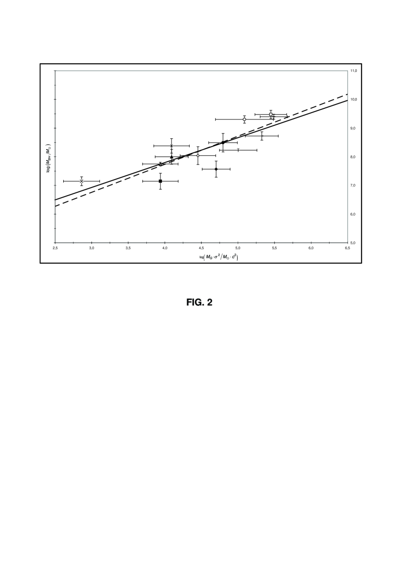
Figure 2: SMBH mass versus $M_{G}\sigma^{2}/c^{2}$ of the host elliptical galaxy. The solid line is the best linear fit (10) with the least squares method, the dashed line is the best fit (12) with the Akritas - Bershadi method [23]. The error bars for $M_{BH}$ are from [3], for $M_{G}$ are in table 1 and for $\sigma$ are calculated from the upper limit on the relative error of $20\%$ estimated from BLF.

In order to check this hypothesis, we show in Fig. 2 the best-fit of the relation

$$Log(M_{BH})=(0.87\pm 0.17)Log\frac{M_{G}\sigma^{2}}{c^{2}}+(4.33\pm 0.80)$$

with a correlation coefficient $r=0.833$ even better (of course with our data) than the famous relation (6).

We have also tried to consider the role of the total kinetic energy adding the contribution due to the rotation velocity and we obtain:

$$Log(M_{BH})=(0.88\pm 0.18)Log\frac{M_{G}(3\sigma^{2}+V^{2})}{c^{2}}+(3.80\pm 0.92)$$

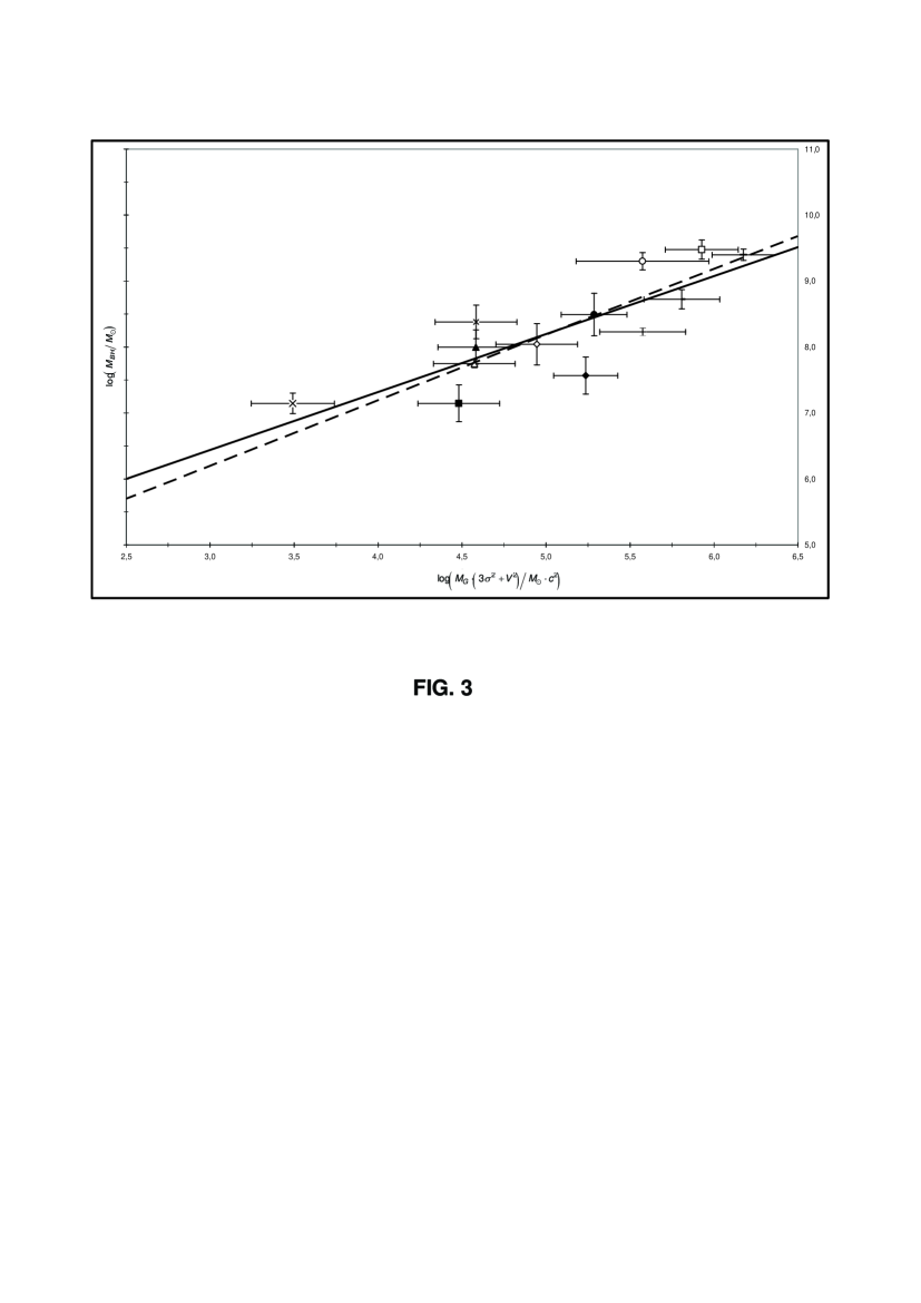
Figure 3: SMBH mass versus $M_{G}(3\sigma^{2}+V^{2})/c^{2}$ of the host elliptical galaxy. The solid line is the best linear fit (11) with the least squares method, the dashed line is the best fit (13) with the Akritas - Bershadi method [23]. The error bars for $M_{BH}$ are from [3], for $M_{G}$ are in table 1 and for $\sigma$ and $V$ are calculated from the upper limit on the relative error of $20\%$ estimated from BLF.

with a correlation coefficient $r=0.829$ and the fit is interesting too (Fig. 3). It is remarkable that the slope of the relation (11) is the same as the relation (10) and that the intercept changes in the way we expect. Furthermore, we can calculate the unknown constant error in $LogM_{BH}$ using (7) and we obtain again $\epsilon_{y}=0.46$ for both the relations (10) and (11) confirming that the procedure leads to a value 2.4 times greater than the average experimental error. So we must check what happens if we use a fit weighted by the experimental errors and take into account also the errors on the independent variable.

As for our kinematical data it is not available the estimate of the error on $\sigma$ for each galaxy, we have considered until now the optimistic assumption of a negligible error. Now it is time to check if something changes in the relation (10), considering the worst scenario of a relative error $20\%$ on $\sigma$ as we can estimate from the discussion on the possible sources of error (anisotropy, triaxiality, fitting procedure, inclination, etc.) contained in BLF. To this aim we use the effective variance method suggested by Orear [22] that with an iterative procedure minimize the $\chi^{2}$ given by the formula

$$\chi^{2}=\sum_{i=1}^{N}\frac{(y_{i}-\alpha-\beta x_{i})^{2}}{(\Delta y_{i})^{2}+\beta^{2}(\Delta x_{i})^{2}}$$

for a relation of the form $y=\alpha+\beta x$. The corresponding results are listed in Appendix A and show no change in the slope of the relationships found until now, the only advantage being a decrease of the difference between the residuals and the corresponding experimental errors. On the contrary, slightly different slopes are obtained starting from the Akritas and Bershadi [23] statistical method (used also in [1]) with the corresponding $68\%$ confidence interval:

$$Log(M_{BH})=(0.98\pm 0.09)Log\frac{M_{G}\sigma^{2}}{c^{2}}+(3.8\pm 0.4)$$

with a reduced $\chi^{2}$ (see Appendix A) $\chi^{2}_{r}=1.9$.

This fit is shown in fig. 2 with a dashed line and involves $M_{BH}c^{2}\propto M_{G}\sigma^{2}$ and could be considered as interesting as the famous relation (1) is.

The same check for the relation (11) gives

$$Log(M_{BH})=(0.995\pm 0.082)Log\frac{M_{G}(3\sigma^{2}+V^{2})}{c^{2}}+(3.21\pm 0.42)$$

(dashed line in fig. 3) with $\chi^{2}_{r}=1.8$.

Even better results can be obtained using a reduced sample (hereafter SAMPLE B) of galaxies if we eliminate the two ellipticals with the largest residuals N821 and N4697. The relationships obtained applying the fitting procedure to the remaining 11 galaxies are listed in Appendix B. The satisfying results are the increase of all correlation coefficients, the decrease of all the values of $\chi^{2}_{r}$ and the slopes of the two relationships that involve the kinetic energies that are closer to the unity. While a coefficient less than one is more difficult to be interpreted, it would be more interesting from the theoretical point of view, the meaningful possibility of a direct proportionality between the mass of a SMBH and the kinetic energy of random motions of the host galaxy. Moreover, if our results are confirmed, the relation between $M_{BH}$ and $M_{G}$ will be non linear [6] [25].

The standard scenario of a Black Hole life predicts that a part of the total mass of a SMBH is due to the accretion process and a part of this last mass can be converted in radiation and ejected again in the region surrounding the Hole. From our results it seems that a part of the rest energy of the Black Hole is in this way strictly related to the kinetic energy of random motions of the stars of the host galaxy even in a region far from the Hole.

4 Conclusions

From our sample of data we derive the suggestion to consider a relationship between the masses of SMBHs and the Kinetic Energy of random motions, or even the total kinetic energy, in elliptical galaxies. Only a deeper analysis with the sophisticated machinery today available and with new data [26], could discriminate if our interpretation can work and if it is generally valid or it holds only for a restricted sample of galaxies (for example the ellipticals with the mass in a small range of values). Given the assumptions of the model, it is clear that triaxiality, anisotropy of the velocity field, inclination, deviations from the $r^{1/4}$ law, are all sources of possible errors that could affect the derived kinematical parameters. In BLF some of these errors were discussed in detail and their total influence on the final results was estimated in no more than $20\%$. However the underestimation of one of the above effects, the restricted sample and even the way to compute the masses we used, can lead to draw wrong conclusions. On the other side we think that it would be surely worse to neglect a priori the suggestion that comes to us by the relationships from (10) to (13) and above all from (10B) to (13B). So we have now arguments to ask again the question contained in the title: is there a relationship between the mass of SMBH and the kinetic energy in its host elliptical galaxy?

Appendix A

The formula used in this paper to estimate all the maximal errors in the functions F of the parameters $(a,b,c,....)$ shown in table 1, is

$$\Delta F(a,b,c)=\left|\frac{\partial F}{\partial a}\right|\Delta a+\left|\frac{\partial F}{\partial b}\right|\Delta b+\left|\frac{\partial F}{\partial c}\right|\Delta c$$

but our results do not change if we use for example the formula of Ferrarese and Merritt [1] (cited also by Tremaine et al. [3]) to estimate the error bar in $LogM_{BH}$ that is

$$\Delta LogM_{BH}=\frac{LogM_{BH(upper)}-LogM_{BH(lower)}}{2}$$

In order to compare our results with the ones obtained by [1], we have used in (12) and (13) the same fitting method [23] and the reduced $\chi^{2}$ given by the formula:

$$\chi^{2}_{r}=\frac{1}{N-1}\sum_{i=1}^{N}\frac{(y_{i}-\alpha-\beta x_{i})^{2}}{(\Delta y_{i})^{2}+\beta^{2}(\Delta x_{i})^{2}}$$

for a relation of the form $y=\alpha+\beta x$. On the other side, the results obtained using the iterative procedure [22] (the errors $\Delta x_{i}$ are ignored in the first step) are the following:

$$LogM_{BH}=(4.10\pm 0.73)Log(\sigma/200)+(8.41\pm 0.12)$$

with $\chi^{2}_{r}=1.1$;

$$LogM_{G}=(2.15\pm 0.38)Log(\sigma/200)+(10.97\pm 0.06)$$

with $\chi^{2}_{r}=3.0$;

$$Log(M_{BH})=(0.88\pm 0.06)Log\frac{M_{G}\sigma^{2}}{c^{2}}+(4.30\pm 0.46)$$

with $\chi^{2}_{r}=2.2$;

$$Log(M_{BH})=(0.89\pm 0.07)Log\frac{M_{G}(3\sigma^{2}+V^{2})}{c^{2}}+(3.77\pm 0.52)$$

with $\chi^{2}_{r}=2.1$.

Appendix B

We neglect the two ellipticals with the largest residuals: N821 and N4697. The relationships contained in the main part of the paper are reanalyzed using the remaining 11 galaxies forming the so called SAMPLE B. The results obtained using the iterative procedure [22] are the following:

$$LogM_{BH}=(4.06\pm 0.73)Log(\sigma/200)+(8.46\pm 0.13)$$

with a linear correlation coefficient $r=0.846$ and $\chi^{2}_{r}=0.9$;

$$LogM_{G}=(2.26\pm 0.52)Log(\sigma/200)+(10.90\pm 0.09)$$

with $r=0.755$ and $\chi^{2}_{r}=1.6$;

$$Log(M_{BH})=(0.92\pm 0.07)Log\frac{M_{G}\sigma^{2}}{c^{2}}+(4.25\pm 0.49)$$

with $r=0.907$ and $\chi^{2}_{r}=0.9$;

$$Log(M_{BH})=(0.92\pm 0.07)Log\frac{M_{G}(3\sigma^{2}+V^{2})}{c^{2}}+(3.70\pm 0.55)$$

with a $r=0.907$ and $\chi^{2}_{r}=0.9$.

The results obtained using the Akritas and Bershadi method [23] are the following:

$$Log(M_{BH})=(1.03\pm 0.08)Log\frac{M_{G}\sigma^{2}}{c^{2}}+(3.71\pm 0.38)$$

with $\chi^{2}_{r}=1.06$;

$$Log(M_{BH})=(1.06\pm 0.08)Log\frac{M_{G}(3\sigma^{2}+V^{2})}{c^{2}}+(3.02\pm 0.39)$$

with $\chi^{2}_{r}=1.01$.

Figure 1: SMBH mass versus luminosity weighted, line of sight velocity dispersion of the host elliptical galaxy. The solid line is the best linear fit with the least squares method (6). The error bars for $M_{BH}$ are from [3] and for $\sigma$ are calculated from the upper limit on the relative error of $20\%$ estimated from BLF.

References

- [1] L. Ferrarese and D. Merritt, ApJ. 539, L9 (2000).
- [2] K. Gebhardt et al., ApJ. Lett. 539, 13 (2000).
- [3] S. Tremaine et al., ApJ. 574, 740 (2002).
- [4] J. Kormendy and D. Richstone ARA & A33, 581 (1995); D. Richstone et al. Nature 395 A14 (1998); R. P. van der Marel in Galaxy interactions at Low and High Redshift Proc. IAU Symposium 186 eds. D. B. Sanders and J. Barnes (Kluwer Academic Publishers, 2000).
- [5] J. Magorrian et al., Astron. J. 115, 2285 (1998); D.Merritt and L. Ferrarese, in The Central kpc of Starbursts and AGN APS Conference Series, vol. 249 eds. J.H. Knapen, J.E. Beckman, I. Shlosman and T.J. Mahoney, (San Francisco: Astronomical Society of the Pacific, 2001) p.335; A. Marconi et al. in Galaxies and their Constituents at the Highest Angular Resolutions, Proc. IAU Symposium 205, ed. R.T.Schilizzi (2001) p. 58.
- [6] L. Ferrarese, ApJ. 578, 90 (2002).
- [7] B.R. McNamara et al., Nature 433, 45 (2005)
- [8] see for example M.G. Haehnelt and G. Kauffmann MNRAS 318, L35 (2000); F.C.Adams, D.S. Graff and D.O. Richstone ApJ. 551, L31 (2000); V. I. Dokuchaev and Yu. N. Eroshenko, arXiv:astro-ph/0209324.
- [9] A. Burkert and J. Silk, ApJ. 554, L151 (2001).
- [10] G. Busarello, G. Longo and A. Feoli, Nuovo Cimento B 105, 1069 (1990).
- [11] S. Chandrasekhar 1969, Ellipsoidal Figures of Equilibrium, (Yale University Press: New Haven and London, 1969).
- [12] G.Busarello and G.Longo in Morphological and Physical Classification of Galaxies eds. G.Longo et al. (Kluwer Academic Publishers, 1992) p.423; G. Busarello, G. Longo and A. Feoli, ”Angular momenta, mass-to-light ratios and formation of elliptical galaxies” Preprint 1994.
- [13] J. Binney and S. Tremaine, Galactic dynamics, (Princeton University Press: Princeton, New Jersey, Third printing 1994) p. 209 and references therein.
- [14] G. Busarello, G. Longo and A. Feoli, Astron. and Astrophys. 262, 52 (1992) (BLF).
- [15] Y. Mellier and G. Mathez, 1987, Astron. and Astrophys., 175, 1 (1987)
- [16] A. Curir, F. De Felice, G. Busarello and G. Longo, Astrophys. Lett. and Commun.28, 323 (1993).
- [17] see also F. Bertola and M. Capaccioli, ApJ 200, 439 (1975); J. Binney and S. Tremaine, Galactic dynamics, (Princeton University Press: Princeton, New Jersey, Third printing 1994) p. 205.
- [18] M. Franx, G. Illingworth and T. Heckman ApJ 344, 613 (1989).
- [19] M. Franx and G. Illingworth ApJ. Lett. 327, L55 (1988).
- [20] T.M. Heckman et al., ApJ., 613 109 (2004).
- [21] D.Merritt, Structure, Dynamics and Chemical Evolution of Elliptical Galaxies eds. I.J. Danziger, W.W. Zeilinger and K. Kjär (ESO, Munich, 1993) p.257.
- [22] J. Orear, Am. J. Phys. 50 912 (1982).
- [23] M.G. Akritas and M. A. Bershadi, ApJ. 470 706 (1996).
- [24] G. Busarello, M.Capaccioli, S.Capozziello, G.Longo and E.Puddu, Astron. and Astrophys., 320 415 (1997).
- [25] A. Laor, ApJ, 553 L677 (2001).
- [26] see for example: N. Haering and H. Rix ApJ Lett. 604 L89 (2004) and, for early type galaxies, J. Pinkney et al., ApJ 596 903 (2003).