The Bright Ages Survey. I. Imaging Data

Abstract

This is the first paper in a series presenting and analyzing data for a K-selected sample of galaxies collected in order to identify and study galaxies at moderate to high redshift in rest-wavelength optical light. The sample contains 842 objects over 6 separate fields covering 75.6 arcmin² down to K=20-20.5. We combine the K-band with UBVRIzJH multi-band imaging, reaching depths of R$\sim$26. Two of the fields studied also have deep HST WFPC2 imaging, totaling more than 60 hours in the F300W, F450W, F606W, and F814W filters. Using artificial galaxy modeling and extraction we measure 85% completeness limits down to K=19.5-20, depending on the field examined. The derived K-band number counts are in good agreement with previous studies. We find a density for Extremely Red Objects (EROs; R-K$>$5) of 1.55$\pm$0.16 arcmin^-2 for K$<$19.7, dominated by the 1714+5015 field (centered on 53w002), with an ERO number density more than 3 times that of the other sample fields. If we exclude the counts for 1714+5015, our density is 0.95+/- 0.14 arcmin. Both ERO densities are consistent with previous measurements due to the significant known cosmic variance of these red sources. Keck spectroscopic redshifts were obtained for 18 of the EROs, all but one of which are emission galaxies. None of the EROs in the 1714+5015 field for which we obtained spectroscopic redshifts are associated with the known $z$=2.39 over-density, although there are three different galaxy redshift pairs ($z$=0.90, $z$=1.03, $z$=1.22).

1 Introduction

Great advances in mapping the high redshift universe have been made, largely through optically selected surveys, such as the Canada France High Redshift Survey(Lilly et al., 1996), Hubble Medium Deep Survey (Ostrander et al., 1998; Ratnatunga et al., 1999), and the Deep Extragalactic Evolutionary Probe (Coil et al., 2004; Madgwick et al., 2003) out to $z\approx 1$, and surveys of Lyman break-selected galaxies beyond z=2 (Madau et al., 1996; Steidel et al., 1999, 2004; Adelberger et al., 2005). Luminosity density and star formation rate increase with redshift, reaching a maximum approximately at redshift 1 – 2.5, what could be labeled as “the Bright Ages”. Star formation density then remains relatively flat out through z=4, with evidence building for a drop out to z=6 (Giavalisco et al., 2004; Bunker et al., 2004; Bouwens et al., 2004a) and beyond (Bouwens et al., 2004b).

One problem with optically-selected high-redshift surveys is that they are biased against the discovery of red galaxies and fall especially short in the search for old and/or reddened star forming galaxies at $z>1.5$. A red galaxy must be an order of magnitude brighter in the rest wavelength optical than a blue galaxy to be included in typical optical high redshift surveys (e.g., Francis, Woodgate, & Danks, 1997). A new generation of deep near-infrared selected surveys were undertaken with the aim of addressing this shortcoming. The Las Campanas Infrared Survey (McCarthy et al., 2001), K20 Survey (Cimatti et al., 2002a), FIRES (Franx et al., 2000), and GOODS (Giavalisco et al., 2004) are sensitive to rest-wavelength optical light even at high redshift, mitigating the problems of reddening and sensitivity to passively evolving populations at high redshift.

Surveys that base their selection on near infrared data are capable of finding substantial numbers of red galaxies at high-redshift (Labbé et al., 2003; Abraham et al., 2004; Fontana et al., 2004), including both dusty starbursts and evolved stellar populations. There is mounting evidence that dust plays a significant role at high redshifts (Rowan-Robinson et al., 1997; Smail et al., 2002; Elbaz et al., 2002), causing high extinction in the rest ultraviolet; as a consequence many of these galaxies drop from optical surveys. Ultraviolet flux is not a reliable star formation indicator, requiring highly uncertain corrections (i.e., Calzetti, 1997; Dickinson, 1997; Tresse & Maddox, 1998) and saturating at the highest luminosities ($\sim$10¹⁰ L_☉; Martin et al., 2005). Rest-frame ultraviolet is also typically dominated by recent starbursts, which can be only a small percentage of the total galactic mass (i.e.,. Shapley et al., 2005).

The commissioning of new telescopes and spectrographs has made the study of infrared-selected samples a very active field. Our survey was constructed so as to take advantage of archival HST imagery reaching to nearly the depth of the Hubble Deep Field, as well as fields containing quasars and clustered CIV absorbers with redshifts placing them in the target $z\sim 2$ bright ages interval. Progress has been dramatic in this subject area, and in recent years we have seen results from the K20 project (Mignoli et al., 2005) with its survey area of $\sim 52$ arcmin²) and the GOODS survey (Giavalisco et al., 2004) of $\sim 300$ arcmin².

Our survey has distinct characteristics: we have multicolor data in six widely separated fields, five of which have evidence of clustering (either CIV absorption system or emission line galaxies) at $z\sim 2.5$. Thanks to our photometric and spectroscopic redshifts, these dispersed fields are studied over a wide slice of redshift space and their physical separation makes our overall results less sensitive to cosmic variance while giving an idea of how important clustering is to contributing to cosmic variance. Further, our field size is well matched to followup with the Keck LRIS spectrograph (Oke et al., 1995) which has recently been upgraded to achieve high sensitivity down to the atmospheric cutoff, a feature of special advantage in measuring Ly alpha emission line redshifts in the $z>2$ Bright Ages. Consequently, our sample enjoys a relatively large number of such galaxies with spectroscopic redshift measurements relative to most such studies; the spectroscopy is discussed in Paper II.

This is the first in a series of papers, which describes the target field selection, creation of K-selected sample, multi-band imaging, photometry, and a discussion of extremely red objects (EROs). Paper II discusses the spectroscopy, determination and testing of photometric redshifts, and the subsequent analysis of luminosity functions, dust extinctions, and star formation density. The assumed cosmology is an $\Omega_{M}$=0.3, $\Omega_{\Lambda}$=0.7 universe with H_o=70 km s^-1 Mpc^-1.

2 Target Fields

Our choice of target fields is based on the presence of already known high redshift sources, particularly where multiple detections at a similar redshift point towards a possible over density or proto-cluster.

The correlation between associated galaxies and high redshift radio galaxies and QSOs has been long known and established from $1<z<5$. Many QSO metal absorption line systems are clustered on comoving scales of $<100h^{-1}Mpc$ or less (Jakobsen et al., 1986; Sargent & Steidel, 1987; Quashnock & Stein, 1999). Malkan, Teplitz, & McLean (1996) demonstrate that targeting such metal absorption-line “clusters” yields the discovery of star-forming galaxies in emission. Further work (Teplitz, Malkan, & McLean, 1998; Mannucci et al., 1998; Meyer, Thompson, & Mannucci, 2003), has continued to discover high-redshift galaxies using this sort of search method. There is also a correlation between CIV absorbers and Lyman Break Galaxies (Adelberger et al., 2003), which presently make up the majority of known high-redshift galaxies. Overdensities of Extremely Red Objects (EROs) are found near radio galaxies (Cimatti et al., 2000) and QSOs (Wold et al., 2003). Recently, a cluster of H-alpha emitters was found in association with a $z=2.16$ massive radio galaxy (Kurk et al., 2004); beyond redshift 4, Lyman alpha emitters are found to be associated with QSOs (e.g. Venemans et al. (2004); Miley et al. (2004)).

Two of our fields are selected from Quashnock, Vanden Berk, & York (1996), who searched their database of heavy-element absorbers to identify nine “superclusters” of multiple CIV absorption systems. The QSO 0149+336 shows four absorbers around a redshift of $z$=2.16, while the QSO 2359+068 has two groups of six absorbers around the redshifts of $z$=2.83 and $z$=2.87. We chose the field near QSO 0953+549 because of multiple known emission candidates at $z$=2.5 (Malkan, Teplitz, & McLean, 1996; Teplitz, Malkan, & McLean, 1998). Similarly, the 1714+5015 field contains a possible $z$=2.39 protocluster of galaxies found in WFPC2 4100Å narrow band imaging (Pascarelle et al., 1996). Finally, in an effort to sample possible over-densities throughout the whole redshift range of $z$=1–3, we include the target field 0741+652, which contains three emission line objects found by the NICMOS parallel grism survey at redshifts $z$=1.33, 1.61, & 1.86 (McCarthy et al., 1999).

One field, 1107+7239, has no known high redshift sources, but has been included because of its deep WFPC2 and NICMOS data, providing a combination of depth, photometric accuracy, and morphological information essentially impossible to obtain from the ground. Between the 1107+7239 and 1714+5015 fields, we have more than 100 hours of Hubble Space Telescope archival imagery; these fields are each roughly half the exposure time of the original Hubble Deep Field. The field locations, references, redshifts, and type of possible over-density are listed in Table 1.

3 Optical Imaging Data

Our optical imaging is obtained from three sources: the UCO/Lick Observatory Shane 3-m Prime Focus Camera, the Keck Observatory Low Resolution Imaging Spectrometer (LRIS), and the Hubble Space Telescope Wide Field/Planetary Camera (WFPC2). A journal of observations, listing all targets, dates, and observation times is given in Table 2.

Optical imaging using the UCO/Lick Observatory Shane 3-m Prime Focus Camera (PFCam) was taken over 14 nights from December 1998 to May 2002. We took deep B, V, R, and I images of 5 of our 6 target fields, only skipping 0953+549 because of Keck LRIS data already in hand. For the September run in 1999, a “Spinrad” R filter was substituted for the more standard Kron-Cousins R, but that data were used only for cross-checking absolute calibration and is not included in the final sample. The PFCam detector is a SITe 2048$\times$2048 thinned CCD with 24-micron (0.296$\arcsec$) pixels, giving a field of view of 9.8$\times$9.8 arcminutes.

The W.M. Keck Observatory Low Resolution Imaging Spectrometer (LRIS; Oke et al., 1995) instrument has two detectors. The red side, or LRIS-R, consists of a backside-illuminated Tek 2048$\times$2048 CCD detector with an imaging scale of 0.215 arcsec/pixel and a field of view of 6$\times$7.3 arcmin. All LRIS observations before June 2002 and all V, R, I, and $z^{\prime}$ filter observations used LRIS-R. The blue side, or LRIS-B, consists of two 2048$\times$4086 Marconi CCDs with extremely high sensitivity in the blue (Q.E. $\sim$90% at 4000Å) with an imaging scale of 0.135 arcsec/pixel. While matched to the red side, the LRIS-B field of view is actually slightly larger at 6$\times$8 arcminutes, but does contain a 13.5 arcsecond gap through its center from an internal bar that is blocking light. It is sensitive over the wavelength range 3100-6000 Angstroms. All U filter observations and 2003 B filter observations were made with LRIS-B. The majority of the observations were made using the 560 dichroic, which splits the light between the two detectors at 5600Å, although the September 2002 run used the 4600Å dichroic and the August 2003 run used the 6800Å dichroic.

Flat fields were produced from combinations of bias-subtracted twilight sky flats and images taken throughout the night. For I and $z^{\prime}$ images, twilight flats could not be used because of the large spectral change in sky at those wavelengths at twilight, so flats came from images alone. Calibration was done by measuring multiple Landolt standard stars in a single field at air masses similar to the observations. For the $z^{\prime}$ filter, standard star magnitudes are calculated using the formula of Smith et al. (2002):

$$z^{\prime}=V-0.841(V-R)-1.65(R-I)+0.51$$ (1)

This produces an AB magnitude which can then be converted to a Vega magnitude using the formula $z^{\prime}$(Vega) = $z^{\prime}$(AB) - 0.54.

As a consistency check, we compare the derived zero points for fields and filters in which both LRIS and PFCam data were taken by comparing multiple (20+) moderately bright stars or compact objects between the two. In the ten combinations of fields and filters where this occurred, the difference is never more than 0.14 magnitudes and generally (7 of 10) 0.1 magnitudes or less. Considering the effects of different seeing and object size (there are generally few bright, unsaturated stars), the two sets of derived zero points appear entirely consistent. As a final check of the absolute calibration of our photometry, we compare our data to the online Sloan Digital Sky Survey Data Release 1 (SDSS DR1) catalog. One of our fields, 0953+549 partially overlaps with the DR1. Although their magnitudes had to be converted from $u^{\prime}g^{\prime}r^{\prime}i^{\prime}$ to UBVRI using Smith et al. (2002), we again find consistency to within 10% for all filters.

The Keck LRIS seeing ranges from 0.7-1.4 arcseconds, with the bulk around 0.9-1.0$\arcsec$, while the Lick PFCam seeing ranges from 1.1-2.0 arcseconds, with typical values around 1.3-1.6$\arcsec$. Because seeing varies widely, a single aperture magnitude limit would be misleading. Instead the magnitude limit is a 5-$\sigma$ detection within an aperture 1.3 $\times$ FWHM, a size found to produce a superior signal-to-noise ratio for a typical compact, faint detection. Not surprisingly, the Keck LRIS magnitude limits are significantly deeper, providing roughly a 2 magnitude advantage across all filters they share in common, with LRIS limits of B$\sim$27, V$\sim$27, R$\sim$26, and I$\sim$25 compared to PFCam limits of B$\sim$25, V$\sim$25, R$\sim$24, and I$\sim$23.5. Also, in 40 minutes on LRIS the images reach depths of $\sim$26 in U and $\sim$25 in $z^{\prime}$ (Vega). All magnitude limit and seeing information, on a field by field basis, is available in Table 3.

3.1 WFPC2 Data

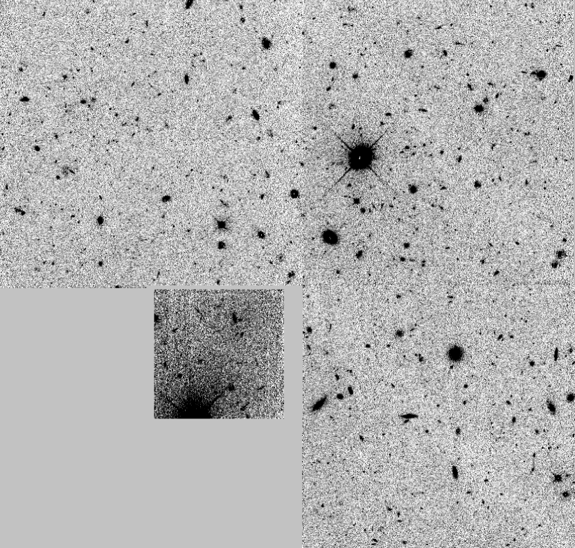
Figure 1: Greyscale F606W image of the 1107+7239 field.

Two of our target fields contain deep pointings using the Hubble Space Telescope Wide Field/Planetary Camera (WFPC2). The 1714+5015 field, also referred to as the Hercules Deep Field, is centered on the $z=2.39$ radio galaxy 53w002 and represents some of the first ultra-deep imaging with the refurbished WFPC2, taken under the GO programs 5308 and 5985 (PI: R. Windhorst) in May 1994 and June 1995. The deep narrow-band imaging in this field revealed 18 associated galaxies appearing to be at nearly the same redshift, thought to be protogalactic clumps that might eventually merge (Pascarelle et al., 1996). The second field, 1107+7239, was observed in April 1998 by R. Edelson and M. Malkan in parallel with a Seyfert galaxy monitoring campaign (NGC 3516; GO program 7355), producing adjacent deep NICMOS and WFPC2 fields over 43 orbits taken within HST’s continuous viewing zone. We present the 1107+7239 WFPC2 image in Figure 1.

The WFPC2 detector consists of four separate CCDs, the three wide field cameras (WFC1,2,3) with a 0.1 arcsecond pixel scale and the planetary camera (PC) with a 0.05 arcsecond pixel scale, which together make the distinctive chevron shape. One major drawback of the WFC chips is that while they have greater sensitivity than the PC chip, they undersample the image, resulting in a loss of resolution. To regain some of that resolution we used variable-pixel linear reconstruction, known more commonly as drizzling (See DITHER/DRIZZLE web page at www.stsci.edu and Fruchter & Hook (2002)).

We drizzled all four 1107+7234 images: F300W, F450W, F606W, and the F814W filters. All the 1107+7234 data are composed of multiple pointings, ranging from 7-12, each with a small rotation in the telescope around the primary NGC 3516 STIS target, with many fractional pixel shifts. All drizzling was done with the IRAF/STSDAS dither package and in an identical manner. We aligned the images by producing a cross-correlation for the WFC chips with the greatest number of bright objects and then used those offsets to calculate the position of the other three chips. This was especially useful for the F410M PC chip image and the 1107+7234 F300W PC, WFC1, and WFC3 images, which did not have enough signal on an individual image for cross-correlation. We drizzled the images from each of the detectors onto a single large image with a pixel scale of 0.05 arcseconds for the 1714+5015 field and 0.04 arcseconds for 1107+7234, the difference being the higher inherent resolution of the F300W data. The only other difference between the reductions for the two fields was the necessity to correct for rotation while calculating the offsets of the 1107+7234 data.

The F606W and F814W images from the 1714+5015 field were generated using only two pointings (and only one pointing in the case of the single F606W offset field) and are therefore not suitable for drizzling. Instead the final images were produced using standard tools in the IRAF/STSDAS, removing cosmic rays, bad pixels (from data quality file), and warm pixels (hot pixels recorded by Space Telescope after every decontamination) from the already pipelined images before combining into a final image. In a few cases bad pixels overlapped, leaving a few bad spots in the final image, but generally the final image quality was excellent. We then created both drizzled and non-drizzled versions of the F450W and F410M images from their four separate pointings. The drizzled versions were matched to each other, while the non-drizzled images were matched to F606W and F814W.

Observations of the 1714+5015 field include 16 hours of integration in F450W, 5.7 hours in F606W, and 5.7 hours in F814W. This can be compared to 33.5 hours, 30.3 hours, and 34.3 hours in the same filters for the Hubble Deep Field (Williams et al., 1996). We ran SExtractor V.2.0.19 (Bertin & Arnouts, 1996) on a combined image produced from a weighted average of the three wide filter images (F450W, F606W, & F814W), selecting objects with 5 connected pixels of 1.5-$\sigma$ each, except for the planetary camera (PC) chip where 9 connected pixels were required. Magnitudes were determined using a 0.5$\arcsec$ aperture, producing 5-$\sigma$ detections limits of 28.5, 28.4, and 27.1 for the F450W, F606W, and F814W filters respectively. Added to this are a second F606W field (a 2 hour integration) immediately south of the prime field and 18 hours of imaging in the narrow-band filter, F410M.

Observations of the 1107+7239 field include 9 hours in F450W, 3.9 hours in F606W, 3.9 hours in F814W, and 24.3 hours in F300W (which is almost 2/3 of the Hubble Deep Field integration in that crucial filter). For this field we required 11 connected pixels of 1.5-$\sigma$ each, as the 1107+7234 image was drizzled, requiring more connected pixels to avoid spurious detections. Magnitudes were also determined with a 0.5 arcsecond aperture, producing 5-$\sigma$ detection limits of 26.1, 27.9, 27.8, and 27.0 for the F300W, F606W, and F814W filters respectively.

4 Near-Infrared Data

The bulk of the infrared observations were done with the UCLA Gemini Twin-Arrays Infrared Camera (McLean et al., 1993) on the UCO/Lick Observatory Shane 3-m telescope. Using a dichroic beam-splitter, this infrared camera images in two filters simultaneously with two separate detectors. The short wavelength camera operates from 1-2.4 $\mu$m using a Rockwell NICMOS3 HgCdTe array, while the long wavelength side operates from 2-5 $\mu$m with its SBRC InSb array. Both detectors are 256$\times$256 pixels in size, with a scale of 0.68 arcseconds per pixel, for a field of view nearly three arcminutes on a side. For all observations, either the J or H filter was used on the short wavelength side, while simultaneously imaging in the K’ filter ($\lambda_{c}$= 2.1235, $\Delta$ $\lambda$ / $\lambda$ = 0.16). We carried out all observations over 13 nights from December 1998 to March 2002, using 9-point dithers and multiple co-adds.

Additional observations of the 0953+549 field were made from June 3-4, 2001, at the Kitt Peak National Observatory (KPNO) Mayall 4-meter telescope with the NOAO Simultaneous Quad Infrared Imaging Device (SQIID; Ellis et al., 1992). Using a series of dichroics and flat mirrors, the SQIID instrument separates the incoming beam into four separate wavelength channels: J, H, K, and L’. Each channel illuminates a separate 512$\times$512 quadrant of a 1024$\times$1024 ALADDIN InSb infrared array, allowing simultaneous observations in all four filters. The sky background at L’, however, is simply too high to allow measurement of the high-redshift objects in this study. While at the f/15 focus of the 4-m, the SQIID pixel scale is 0.39$\arcsec$ per pixel, with an un-vignetted field of view of 2.9$\times$3.0 arcminutes in each channel.

For infrared imaging of the 1714+5015 field we used the MDM/Ohio State Array Infrared Camera (MOSAIC Pogge et al., 1998), which is also referred to as TIFKAM or ONIS (Ohio State/NOAO Imaging Spectrograph), at the MDM Hiltner 2.4-m telescope. The MOSAIC used a 512$\times$1024 InSb array with a pixel scale of 0.30$\arcsec$ per pixel at the f/7 focus of the 2.4-m, providing a field of view of approximately 5.12$\times$2.56 arcminutes. The observations were made on seventeen nights between May 12, 1998 and July 1, 1999. We used three different filters: J_Barr ($\lambda_{c}$=1.267$\mu$m, FWHM=0.271$\mu$m), H_Barr ($\lambda_{c}$=1.672$\mu$m, FWHM=0.274$\mu$m), and K_Barr ($\lambda_{c}$=2.224$\mu$m, FWHM=0.394$\mu$m). Total integration times for the three filters were 6.18, 5.23, and 16.03 hours, respectively. The observations are divided into two pointings, an east field and a west field, each roughly one arcminute apart. This gives a central region in the final image, approximately 1.8$\arcmin$ $\times$ 5$\arcmin$ with twice the integration time of the outer regions. Combining both low and high signal-to-noise ratio regions gives an area of 16.2 arcmin² down to K=20.5 or better.

Images were flat-fielded using a median of all data from each night, while sky frames were created from medians of the data taken immediately before and after. This process, similar, if more critical, to that done to the optical PFCAM data, can also lead to faint, negative images near bright objects in the final image. After sky subtraction and flat-fielding, stars on each frame are examined to determine the relative signal-to-noise ratio and seeing, which were used to produce weights for averaging, and the general photometric quality of the data. Particularly bad frames (bad sky subtraction, a bias or dark fluctuation, tracking loss, cloud passing overhead, planes passing overhead, etc.) were removed. Finally, the images were masked for known bad pixels, shifted to align bright objects on each frame, and averaged together.

Calibration was done by observing faint UKIRT and Persson et al. (1998) infrared standards throughout the night at air masses similar to the observations. The K’ calibration is interpolated from the J, H, and K standard magnitudes, but it is only 0.01-0.04 magnitudes different than assuming K magnitudes apply. As a final check of our calibrations, we compared the photometry of our brightest objects against the 2 Micron All Sky Survey (2MASS) photometry maintained by the NASA/IPAC Infrared Science Archive (http://irsa.ipac.caltech.edu). The 2MASS photometric catalog has 10-$\sigma$ point source detections down to at least J=15.8, H=15.1, and K_s=14.3 and contains sources extracted with a signal-to-noise ratio greater than 7 in any one band or signal to noise ratio greater than 5 in any two bands. Objects of this brightness are easily detected in our images, typically 3-4 objects per 3$\times$3 arcminute image. Roughly 35% of the UCLA Gemini fields (J,H, & K’ considered separately), required minor zero point adjustments, roughly 10-15%. The MOSAIC 1714+5015 images, a combination of data across eight nights, required more significant final corrections to the zero points: 0.32, 0.14, and 0.23 magnitudes in the J, H, and K filters respectively. These reductions show that some non-photometric nights were erroneously considered to be photometric at the time of the observations.

Due to unusually high background at time of observation, the SQIID data are slightly shallower than those taken with the UCLA Gemini camera, but with marginally better seeing: $\sim$1.6$\arcsec$. UCLA Gemini seeing is typically 1.8-2.0$\arcsec$, degrading to 2.5$\arcsec$ in a few instances. We combined the 0953+0549 images from the two instruments, weighted by signal-to-noise ratio and seeing, producing a final image with seeing and signal-to-noise ratio superior to the original UCLA Gemini image. The two K filters are not identical: standard K vs. K’. However, the estimated likely K’ differences from interpolated star magnitudes are on the order of 1-4%, so final averaged photometry calibration errors, where the two input images were similarly weighted, should be roughly half of that. This is small compared to most of the photometric errors used, and is deemed acceptable for the signal gain.

Table 4 contains a summary of magnitude depths, image sizes, and seeing for all fields and partial fields. Again, because seeing varies (1-2$\arcsec$), the magnitude limit is a 5-$\sigma$ detection within an aperture 1.3 $\times$ the FWHM. These are not total magnitudes, estimation of which will be covered in more detail below.

In total, we imaged 10 partial near-infrared fields at six different target locations, covering 75.6 arcmin² down to a total K’ magnitude of 20 and 36.3 arcmin² down to K’=20.5 or fainter.

5 Photometry, Completeness, and Infrared Number Counts

We extract 842 K-selected objects from the K and K’ images using the SExtractor V.2.0.19 package (Bertin & Arnouts, 1996), which finds and extracts objects after convolving the field with a Gaussian matching the measured FWHM and subtracting off the remaining background. typical requirement is 9 connected pixels all above 2-$\sigma$. We change this criteria slightly from field to field to ensure selection of objects well below the 5-$\sigma$ aperture limits.

For photometry, SExtractor extracts both a BEST magnitude and an aperture magnitude corresponding to 1.3$\times$FWHM. The BEST magnitude is either a Kron elliptical aperture (Kron, 1980) or isophotal magnitude for blended/crowded objects. The object detection list for each field is then taken and cleaned of spurious bad pixel or noise features, objects clipped by the edges of the image, and bright stars. The stars are determined using the SExtractor CLASS_STAR output parameter and comparison to the actual image. As a final cut, any detection that has an aperture magnitude greater (i.e., dimmer) than the 5-$\sigma$ limits quoted in Table 4 is removed. A distribution of all K-selected objects is shown in Figure 2. Just from examining the turn-over in counts, we can get a rough idea that the typical data is complete to $\sim$19.5, while the deepest data are complete to $\sim$20. For a more rigorous examination of completeness, we examine the extraction of artificial galaxies.

5.1 Creating Artificial Galaxies To Test Completeness and Photometry Extraction

To check completeness and the accuracy of using the SExtractor BEST magnitudes, we create artificial galaxies using the IRAF program MKOBJECTS, available in the noao.artdata package. The program allows selection of ellipticity, half-light radius, profile type, and position angle. From quantitative morphological examination of galaxies in the Hubble Deep Field (Marleu & Simard, 1998), we have detailed distributions of both half-light and eccentricity in the F814W filter down to 26th magnitude (AB). As a simple model, we can break both these distributions into two groups. Looking at half-light radius, 75% have a small r_hl with the distribution peaking around 0.25$\arcsec$ while 25% have a larger r_hl roughly centered at 0.5$\arcsec$. For eccentricity, 75% have a small $e$ around 0.25 while 25% have larger $e\sim$ 0.55. Assuming no correlation between r_hl and $e$, this simple model presents a distribution of galaxies that is 56% small with low eccentricity, 19% small with high eccentricity, 19% large with small eccentricity, and 6% large with large eccentricity. While deep HST imaging finds some differences in morphology between galaxies imaged at 0.8$\mu$m and the near-infrared, such as fewer irregulars, generally both wavelengths show a similar distribution of morphologies (Teplitz et al., 1998). We therefore apply the F814W models to our K’ data, as the relatively minor morphology differences are unlikely to have a significant effect on these sort of simplified distributions.

We create four model galaxies to represent this simplified galaxy distribution: [r${}_{hl},$e$]$ = [0.25,0.25], [0.25,0.55], [0.5,0.25], & [0.5, 0.55]. We choose an exponential disk for the galaxy profile type, as evidence shows that deep galaxy counts are better fit by disk than by bulge models (Marleu & Simard, 1998). However, as roughly 25% of sources at these near-infrared depths are ellipticals (Cassata et al., 2005), we also examine a de Vaucouleurs profile to check how that might change the results. Having created the models, we convolve them with a Moffat point spread function derived from examining stars from the image fields, and scale their fluxes to a series of magnitudes from 18-21 in 0.25 magnitude intervals. Then each model galaxy is placed into the images repeatedly at random locations, and extracted using SExtractor with the exact same parameters and cuts used to extract the final K-selected object lists. This is done for every target field, as there are large field-to-field variations in depth and seeing.

Because of the random placement of the model galaxies, 100% recovery (and therefore completeness), is not possible, even for galaxies a magnitude or two above the limits of the image. There are enough bright and/or large objects to hide 5-15% of the fainter input galaxies in most images. Therefore, to find the magnitude limits at which completeness drops purely because of signal-to-noise ratio effects, one needs to look for an abrupt drop in the recovery rate, where, for example, completeness will drop 20-30% between 0.25 magnitude width bins. With this in mind, we record where completeness drops below 85% for each field. This should roughly correspond to the magnitude depth for 100% completeness, if one had hand-placed all the model galaxies in empty parts of the image. Four of the fields, 1107+7239, 1714+5015 Center, 0149+336 Prime, and 0741+652, show 85% completeness or better down to K=20 and 50% completeness or better down to 20.25. The rest are all 85% complete down to 19.5 or better. Completeness limits are summarized in Table 4. Use of the de Vaucouleurs profile model galaxy produces completeness limits ranging from 0-0.5 magnitudes brighter.

We also examine the accuracy of the BEST magnitudes for this data. We plot the median difference in magnitude between the input exponential disk model magnitude and its extracted BEST magnitude versus the input magnitude in Figure 3. This includes all fields but excludes any data from magnitude bins with less than 55% completeness. The standard deviation of this difference from field to field is represented by the error bars. For all magnitude bins this median difference is less than 0.05 magnitudes and within one standard deviation of zero. We also check the de Vaucouleurs profile, which produces a BEST magnitude which consistently underestimates the total flux of the input magnitude by about 0.15 magnitudes. However, as we expect most galaxies to be better fit by exponential disk profiles, the BEST magnitudes are an accurate measurement of total flux.

5.2 Near-infrared Number Counts

To produce K-band number counts, we combine all the data down to the 85% completeness limit in each field, except for the four deepest fields, where we use data down to the 50% completeness limits. Figure 4 shows the final K number counts for all fields, with and without completeness corrections, plotted with several other deep K number counts from previous studies (McLeod et al., 1995; Minezaki et al., 1998; Saracco et al., 1999; Maihara et al., 2001). The number counts are entirely consistent, generally agreeing well within the error bars, with the exception of the bright end, which is high, and a single bin at 17.25 magnitudes, which is low. Neither are more than 2-$\sigma$ off from the rest. The data also do not support the low number density values at the bright magnitudes from Saracco et al. (1999), which consistently lie below the other studies as well as this one.

6 Combining Near-infrared and Optical Photometry

All other images taken with different filters are matched to the K-band image. To accommodate different pixel scales, the lower resolution images are magnified to match the higher resolution images. Since most of the infrared data is taken at a pixel scale of 0.68$\arcsec$/pixel, this sometimes led to large magnifications, particularly when matched to the LRIS-B 0.134$\arcsec$ or WFPC2 0.1$\arcsec$ pixel scale. In the case of 1107+7239, the WFPC2 data were re-sampled to match a coarser pixel scale (0.298$\arcsec$/pixel), as the drizzled 0.04$\arcsec$/pixel scale would have been too unwieldy. The data are registered to the K-band image by measuring 20-40 objects in common and fitting a second order polynomial to determine the needed transformation between pixel values and sky coordinates.

To match photometry and produce accurate colors, all images are blurred to the same seeing FWHM by convolving the images with a Gaussian. While a Gaussian convolution is not a perfect representation of the seeing, we choose it as a better solution for measuring accurate colors than the adoption of different sized apertures, which cannot entirely account for significant color gradients. Deviations of the Gaussian-convolved images from those effected only by atmospheric seeing are undetectable for small FWHM changes. This does not continue to be true, however, for more extreme convolutions (see WFPC2 matching below).

Typically we blur the data to match the J image, although in a few cases (0953+549 & 0741+652) the final K image has the worst seeing. One J image data from the southern 2359+068 field has grossly substandard seeing (3.4$\arcsec$) and is only included as no other J band data are available. It has been completely removed from the normal matching process, and seeing is matched to the K image instead.

Once all data are registered, magnified, and blurred, we run SExtractor on the original non-blurred K image as described above and use those object detections to extract the photometry from each of the blurred images using an aperture magnitude corresponding to 1.3$\times$FWHM of the final, blurred image. The final magnitudes for each object in each filter are then defined as the K image BEST magnitude plus the difference between the blurred K image aperture magnitude and the blurred aperture magnitude for each filter:

$$N_{final}=K_{original}(BEST)-[K_{Blurred}(Aperture)-N_{Blurred}(Aperture)]$$ (2)

where N is the magnitude in the filter being examined.

One exception to the above procedure is the addition of WFPC2 data to ground-based infrared and optical bands, as we did not wish to blur the WFPC2 images from a FWHM of roughly 0.1$\arcsec$ to 2$\arcsec$. To measure the total WFPC2 magnitudes, we extract the BEST magnitude for all the unblurred F814W objects detected at greater than 5-$\sigma$ in a 0.8$\arcsec$ aperture and apply that same 0.8$\arcsec$ aperture to each of the remaining WFPC2 filters (F606W, F450W, and also F300W for 1107+7239), determining the total fluxes from the aperture differences from F814W. In the rare instance of multiple sources within an arcsecond of each other, we combine their WFPC2 fluxes into a single magnitude, as they would be indistinguishable at the resolution of the infrared data. This method provides accurate colors except in the extreme case of a strong intrinsic galaxy color gradient.

As a final step before producing colors or photometric redshifts, a correction for galactic extinction is made. This uses the galactic extinctions of Schlegel, Finkbeiner, & Davis (1998) as given by the NASA/IPAC Extragalactic Database (NED). While the extinctions at K are essentially negligible (0.002-0.029), this is not the case with the other wavelength extreme, U band, for which extinction can be as high as 0.435 magnitudes. A list of galactic extinction E(B-V) is included in Table 1. We produced color-color diagrams of this final combined photometric data set, which show good agreement with expected stellar tracks (see Paper II for further discussion).

7 Extremely Red Objects

Extremely Red Objects (EROs), first found in early deep K-band imaging (Elston et al., 1988), are sources much brighter in the near-infrared than in the optical. EROs are generally defined as having R-K $>$ 5, although other overlapping criteria (e.g., R-H$>$4, I-K$>$3.5, I₇₇₅-K$>$3.92) have also been used (Firth et al., 2002; Daddi et al., 2003; Roche et al., 2003). These ERO colors are consistent with either an old, passively-evolving stellar population or significantly dust-extincted star formation at moderate to high redshift. The density and nature of these objects has been used to infer either significant quantities of early massive galaxy formation or substantial hidden star formation (Cimatti et al., 2002b; Miyazaki et al., 2003). Complicating matters further, EROs are strongly clustered on the sky, producing a large cosmological variance from field to field. This variance can easily range from factors of 3-6 in surface density for even large near-infrared fields of view (25 arcmin²; Daddi et al., 2000).

We examine this effect by identifying EROs within 5 of our 6 near-infrared fields. We exclude 0149+336 from this analysis because of its relatively shallow optical (Lick only) imagery. The remaining sample contains 481 objects down to a K magnitude of 19.7, covering 61 square arcminutes. We plot R-K versus K in Figure 6. For most fields the filter plotted is actually K’, which will have a negligible impact on the R-K color, unless a break were to fall within the K filter (z$\sim$4 for the 4000Å break). All fields use the same R filter from the Keck LRIS.

We find 95 EROs (R-K $>$ 5; K $<$ 19.7) in our sample for a density of 1.55$\pm$ 0.16 arcmin^-2. This compares well with the density of $1.60\pm 0.09$ found by Georgakakis, A. et al. (2005), adopting $I-K>4$ and $K<20$ in the Phoenix Deep field. The density changes significantly across the five fields, ranging from 0.67-3.3 arcmin^-2, with the largest deviation being the 1714+5015 field which contains slightly more than half (52) of all candidates in only 25% of the observed area. Excluding 1714+5015 produces a density of 0.95$\pm$ 0.14 arcmin^-2. A fluctuation of 5 between fields is within the range of predicted density fluctuations. The 1714+5015 field K-band number counts show no large disparities, within the errors, from the K-band number counts of all the combined fields. The 1714+5015 counts do seem to be slightly higher from K=18.25-19.5, but this is of marginal significance. There is no significant spatial clustering visible within the 3$\times$5 arcminute near-infrared 1714+5015 field image, nor within the other smaller fields with lower ERO density. If we place the magnitude cut-off at K=19.2 to allow easier comparison with previous studies, we measure a density of 1.10$\pm$ 0.13 arcmin^-2. This agrees reasonably well with most previous studies (Daddi et al., 2000; Cimatti et al., 2002b; Firth et al., 2002) that find densities of 0.5-1 EROs arcmin^-2, where our result is slightly high because of the single extreme 1714+5015 field.

A high density of red objects has been previously noted within the 1714+5015 field, with Im et al. (2004) reporting a population of Hyper-EROs (HEROs), objects with J-K $>$ 2.7 believed to be at redshifts of $z>2$ (Im et al., 2002). However, these objects are in general not the EROs we report here, as the HERO population are mostly much fainter (K$>$20.5; Im, M. 2005, private communication). Our study is not sensitive to anything but the brightest HEROs, as much deeper J-band data are required to confirm such extreme near-infrared colors. We further investigate the possibility that the 1714+5015 EROs might be at very high redshift by performing a B-z versus z-K color-color (BzK) analysis, which is capable of selecting both star-forming and passive galaxies at $z>1.4$ (Daddi et al., 2004). We find only 30% of the 1714+5015 ERO sample is above $z=1.4$, evenly distributed between star-forming and old galaxies, which indicates the majority of the EROs are not associated with the known $z$=2.4 over-density (Pascarelle et al., 1996).

We examined the morphologies of those EROs that lay within the 1714+5015 WFPC2 F814W images (12 total). Because they are very faint at optical wavelengths we did not attempt to extract any morphological parameters, as meaningful results require signal-to-noise ratios of 50-100 (ex., Conselice, 2003). The majority (10 of 12) are extremely compact, which we subjectively split into 6 disk-like, 3 spheroid-like, and 3 so compact as to be essentially point-like (although they are resolved). Of the remaining two EROs, one is clearly an elliptical, while the other is an extended disk with arm-like features.

Spectroscopic redshifts were obtained for 18 of the 95 EROs (See Paper II for spectroscopy details), which ranged from z=0.53-2.55 with most lying in the z=0.7-1.2 range. None are obvious AGNs or stars. All but one were identified from emission lines, making them almost all dusty starbursts. This is almost certainly a strong selection effect, as emission spectra are more easily identifiable than absorption spectra, particularly for the reddest objects in our sample. We failed to obtain spectroscopic redshifts for an additional 24 K$<$19.7 EROs, indicating as much as 60% of the ERO sample could be passively evolving. Previous studies have indicate a ratio of passively evolving to dusty star-forming EROs close to 1 (i.e., Cimatti et al., 2002b; Miyazaki et al., 2003). No significant redshift clustering is seen in the ten redshifts measured for the 1714+5015 field to explain the ERO over-density, although there are three different pairs of galaxies at the same redshift (z=0.90,z=1.03,z=1.22), possibly indicating a chance alignment of smaller over-densities.

8 Summary

This paper presents data from the Hubble Space Telescope, three ground observatories, five different telescopes, seven different instruments, eight different fields, and fourteen different wavelength filters, covering the ultraviolet through near-infrared. The combined set of optical and near-infrared photometry, roughly 75 arcmin² down to K=20-20.5, consists of six different fields throughout the sky, greatly reducing the vulnerability to cosmic variance.

From these target fields we extract 842 K-selected sources, producing number counts consistent with previous near-infrared samples. After producing optical through near-infrared colors, we measure an ERO density of 1.55$\pm$ 0.16 arcmin^-2, higher than most previous studies, but within the known variance of near-infrared fields of the size examined. Roughly half of the detected EROs lie within the 1714+5015 field, a field already known to contain an over-density of red galaxies. Spectroscopic confirmations indicate the explanation for the high ERO density in 1714+5015 may not be a single cluster, but a chance alignment of red galaxies at multiple redshifts.

Most major studies of the high-redshift universe have been done in the rest-wavelength ultraviolet, potentially missing a significant redder high-redshift population. Our K-band selected sample allows examination of these redder galaxies out to the Bright Ages ($z$=1-2.5). In Paper II we will discuss the follow-up spectroscopy and detection of a significant number of galaxies at high redshift, allowing the determination of reliable photometric redshifts for study of the evolution of luminosity functions, dust extinction, and star formation density.

We acknowledge assistance from the team that obtained the parallel HST observations of the 1107+7239 field, including the Principal Investigator (R. Edelson), and A. Koratkar for the scheduling and R. Fruchter for a preliminary reduction of some of the data. We would also like to thank Myungshin Im for his valuable input. We am grateful for the work of Ian McLean and the entire UCLA Gemini Twin-Arrays Infrared Camera team, without which this project would not have been possible. We wish to also acknowledge the use of TIFKAM, which was funded by the Ohio State University, the MDM consortium, MIT, and NSF grant AST-9605012. NOAO and USNO paid for the development of the ALADDIN arrays and contributed the array currently in use in TIFKAM. The assistance of the staffs of the Lick, Kitt Peak, and Keck observatories was invaluable. Finally, We would like to acknowledge financial support from a grant for HST program AR-9543.

Table 1: Target Fields

Target Field	RA	Dec	Gal. Ext.	z	Type	Ref.
	(J2000)	(J2000)	E(B-V)
0149+336	01h52m34.6s	+33∘50$\arcmin$33$\arcsec$	0.041	2.16	absorption	A
0741+652	07h41m45.4s	+65∘15$\arcmin$36$\arcsec$	0.033	1.33,1.61,1.86	emission	B
0953+549	09h57m14.7s	+54∘40$\arcmin$18$\arcsec$	0.007	2.50	emission	C
1107+7239	11h06m50.0s	+72∘39$\arcmin$00$\arcsec$	0.043	n/a	deep field	D
1714+5015	17h14m14.7s	+50∘15$\arcmin$30$\arcsec$	0.022	2.39	emission	E
2359+068	00h01m40.6s	+07∘09$\arcmin$54$\arcsec$	0.058	2.83,2.87	absorption	A

References. — A) Quashnock, Vanden Berk, & York (1996) B) McCarthy et al. (1999) C) Teplitz, Malkan, & McLean (1998) D) Deep NICMOS and WFPC2 fields taken in parallel with a STIS observation program of NGC 3516 by Rick Edelson. E) Pascarelle et al. (1996)

Table 2: Journal of Observations

Target Field	Filter	Int. Time	Telescope	Observation Dates
		(Seconds)
0149+336	B	9000	Lick 3m	Oct 2 2000
	V	9000	Lick 3m	Oct 1 2000
	R	6600	Lick 3m	Oct 2,3 2000
	I	7200	Lick 3m	Oct 1,3 2000
	J	18360	Lick 3m	Nov 16,17 2000; Jan 31 2002
	K’	19152	Lick 3m	Nov 16,17 2000; Jan 31 2002
0741+652	U	2400	Keck	Jan 5 2003
	V	1800	Lick 3m	Dec 18 1998
	R	1300	Keck	Jan 5 2003
	I	5400	Lick 3m	Dec 18 1998; Jan 19 2002
	z’	1060	Keck	Jan 5 2003
	J	13320	Lick 3m	Jan 1 1999; Jan 31 2002
	H	6960	Lick 3m	Jan 30 2002
	K’	20306	Lick 3m	Jan 1 1999; Jan 30,31 2002
0953+549	U	2600	Keck	June 11 2002
	B	1800	Keck	Jan 5 1997
	V	2000	Keck	Dec 24 1995
	R	1200	Keck	June 11 2002
	I	3200	Keck	Dec 23 1995; June 11 2002
	J	35280	Lick 3m	Mar 19,21+Nov 16,17 2000
	J	5640	Kpno 4m	June 3,4 2001
	H	5340	Kpno 4m	June 3,4 2001
	K’	35060	Lick 3m	Mar 19,21+Nov 16,17 2000
	K	5460	Kpno 4m	June 3,4 2001
1107+7239	B	1680	Keck	Mar 25 2003
	V	9000	Lick 3m	Dec 17 1998
	R	1500	Keck	Mar 25 2003
	I	7200	Lick 3m	Dec 18 1998
	J	12800	Lick 3m	Jan 1, Mar 1 1999
	H	11988	Lick 3m	Jan 1, Mar 1 1999
	K’	24336	Lick 3m	Jan 1, Mar 1 1999
1714+5015	U	6650	Keck	Sept 13,14 2002; Feb 25 2003
	B	1200	Keck	Feb 25 2003
	V	2200	Keck	Sept 13,14 2002
	R	1200	Keck	Sept 14 2002
	I	1400	Keck	Feb 25 2003
	z’	2250	Keck	Feb 25 2003
	J	22260	MDM 2.4m	May 16,17,19,23,26 1998; June 19+July 1 1999
	H	18840	MDM 2.4m	May 23,26+Oct 8,9,11 1998; July 1 1999
	K’	57720	MDM 2.4m	May 12,14,15,23,24,26 1998; June 18,20 1999
2358+068	U	2650	Keck	Aug 28 2003
	B	9000	Lick 3m	Sept 3 1999
	V	9000	Lick 3m	Sept 7 1999
	R	1000	Keck	Aug. 28 2003
	I	1000	Keck	Aug. 28 2003
	z’	1450	Keck	Aug 29 2003
	J	13320	Lick 3m	Sept 17 1999; Nov 17 2000
	K	13176	Lick 3m	Sept 17 1999; Nov 17 2000

Table 3: Ground-based Optical Field Depths and Seeing

Optical	U 5$\sigma$	B 5$\sigma$	V 5$\sigma$	R 5$\sigma$	I 5$\sigma$	z 5$\sigma$	U ($\arcsec$)	B ($\arcsec$)	V ($\arcsec$)	R ($\arcsec$)	I ($\arcsec$)	z ($\arcsec$)
Field	Lim.	Lim.	Lim.	Lim.	Lim.	Lim.	Seeing	Seeing	Seeing	Seeing	Seeing	Seeing
0149+336	n/a	25.1	25.1	24.1	23.3	n/a	n/a	1.5	1.3	1.3	1.2	n/a
0741+652	26.1	n/a	23.5	26.0	23.6	23.6	1.4	n/a	1.3	1.3	1.3	1.3
0953+549	25.8	27.1	27.3	26.2	25.0	n/a	1.1	1.1	0.8	1.0	0.9	n/a
1107+7239	n/a	26.9	24.4	25.8	23.7	n/a	n/a	1.1	1.7	1.2	1.1	n/a
1714+5015	26.2	26.9	26.4	25.8	25.5	25.0	0.9	0.9	0.9	0.9	0.8	0.7
2359+068	25.8	24.8	24.6	26.0	25.2	24.5	0.9	1.6	1.6	0.9	0.8	0.7

Table 4: Infrared Field Depths, Sizes, and Seeing

Infrared	J 5-$\sigma$	H 5-$\sigma$	K’ 5-$\sigma$	Size	J ($\arcsec$)	H ($\arcsec$)	K’($\arcsec$)	K 85%	Observa-
Field	Limit	Limit	Limit	(arcmin2)	Seeing	Seeing	Seeing	Complete	tory
0149+336 Prime	22.04	n/a	20.88	7.6	2.1	n/a	1.9	20.0	Lick 3m
0149+336 West	21.64	n/a	20.30	6.4	1.9	n/a	1.9	19.5	Lick 3m
0741+652	22.69	21.63	20.97	7.1	1.6	1.7	1.8	20.0	Lick 3m
0953+549 North	22.31	20.94	20.35	8.1	1.9	1.4	2.4	19.5	Lick 3m
0953+549 South	21.70	20.47	20.34	7.5	1.9	1.3	1.8	19.5	Lick 3m
1107+7239	21.67	20.73	20.74	7.7	2.4	1.9	2.0	20.0	Lick 3m
1714+5015 Cent.	22.16	20.94	20.89	8.8	1.2	1.2	1.1	20.0	MDM 2.4m
1714+5015 Sides	21.85	20.52	20.52	7.4	1.2	1.2	1.1	19.5	MDM 2.4m
2359+068 North	21.67	n/a	20.27	7.4	2.2	n/a	2.0	19.75	Lick 3m
2359+068 South	21.16	n/a	20.46	7.6	3.4	n/a	2.0	19.75	Lick 3m

Figure 2: A histogram of all K-selected objects (including objects later classified as stars) from the 6 fields comprising the 75.6 sq. arcmin of this survey.

Figure 3: A distribution of the difference between the extracted BEST magnitude used by SExtractor and the input magnitude of the artificial galaxies created using the exponential disk model, given as a function of the model input magnitude. This plot shows that the BEST magnitude is accurate down to almost 50% completeness, where the average field tested reaches K=20.25.

Figure 4: K-band number counts for our infrared fields. Solid diamonds are our counts, not corrected for completeness; the solid rectangles are the corrected counts. Notice that completeness corrections are significant only for K$>$20 mag. For comparison, K number counts from previous studies are also displayed: the open triangles are from McLeod et al. (1995), the X’s are from Minezaki et al. (1998), the asterisks are from Saracco et al. (1999), and the open squares come from Maihara et al. (2001).

Figure 5: R-K color plotted against K magnitude for all objects with K$>$19.7, excluding field 0149+336 due to the relative shallowness of its optical data. The R-K$>$5 ERO demarcation is drawn as a dashed horizontal line. Lower limits in R-K are indicated with upward pointing arrows. Sources with spectroscopic redshifts are plotted as solid upside down triangles, AGN are plotted as solid squares, and one star (remaining after an initial color cut to remove stars) is plotted as an asterisk.

References

- Abraham et al. (2004) Abraham, R. G., et al. 2004, AJ, 127, 2455
- Adelberger et al. (2005) Adelberger, K. L., Steidel, C. C., Pettini, M., Shapley, A. E., Reddy, N. A., & Erb, D. K. 2005, ApJ, 619, 697
- Adelberger et al. (2003) Adelberger, K. L., Steidel, C. C., Shapley, A. E., & Pettini, M. 2003, ApJ, 584, 45
- Bergeron & Boisse (1991) Bergeron, J. & Boisse, P. 1991, A& A, 243, 344-366
- Bertin & Arnouts (1996) Bertin, E. & Arnouts, S. 1996, A&AS, 117, 393
- Bouwens et al. (2004a) Bouwens, R. J., et al. 2004a, ApJL, 606, L25
- Bouwens et al. (2004b) Bouwens, R. J., et al. 2004b, ApJL, 616, L79
- Bunker et al. (2004) Bunker, A. J., Stanway, E. R., Ellis, R. S., & McMahon, R. G. 2004, MNRAS, 355, 374
- Calzetti (1997) Calzetti, D. 1997, Proceedings of the Conference “The Ultraviolet Universe at Low and High Redshift”
- Cassata et al. (2005) Cassata, P., et al. 2005, MNRAS, 357, 903
- Coil et al. (2004) Coil, A. L., et al. 2004, ApJ, 609, 525
- Cimatti et al. (2000) Cimatti, A., Villani, D., Pozzetti, L., & di Serego Alighieri, S. 2000, MNRAS, 318, 453
- Cimatti et al. (2002a) Cimatti, A., et al. 2002a, A&A, 392, 395
- Cimatti et al. (2002b) Cimatti, A., et al. 2002b, A&A, 381, L68
- Conselice (2003) Conselice, C. J. 2003, ApJS, 147, 1
- Daddi et al. (2004) Daddi, E., Cimatti, A., Renzini, A., Fontana, A., Mignoli, M., Pozzetti, L., Tozzi, P., & Zamorani, G. 2004, ApJ, 617, 746
- Daddi et al. (2003) Daddi, E., et al. 2003, ApJ, 588, 50
- Daddi et al. (2000) Daddi, E., Cimatti, A., Pozzetti, L., Hoekstra, H., Röttgering, H. J. A., Renzini, A., Zamorani, G., & Mannucci, F. 2000, A&A, 361, 535
- Dickinson (1997) Dickinson, M. 1997, STSci May 1997 Symposium “The Hubble Deep Field,” eds. M. Livio, S.M. Fall and P. Madau
- Elbaz et al. (2002) Elbaz, D., Cesarsky, C. J., Chanial, P., Aussel, H., Franceschini, A., Fadda, D., & Chary, R. R. 2002, A&A, 384, 848
- Ellis et al. (1992) Ellis, T. et al. 1992, Proc. SPIE, 1765, 94
- Elston et al. (1988) Elston, R., Rieke, G. H., & Rieke, M. J. 1988, ApJL, 331, L77
- Firth et al. (2002) Firth, A. E., et al. 2002, MNRAS, 332, 617
- Fontana et al. (2004) Fontana, A., et al. 2004, A&A, 424, 23
- Francis, Woodgate, & Danks (1997) Francis, P.J., Woodgate, B.E., & Danks, A.C. 1997, ApJ, 482, L25
- Franx et al. (2000) Franx, M., et al. 2000, The Messenger, 99, 20
- Fruchter & Hook (2002) Fruchter, A. S. & Hook, R. N. 2002, PASP, 114, 144
- Giavalisco et al. (2004) Giavalisco, M., et al. 2004, ApJL, 600, L103
- Georgakakis, A. et al. (2005) Georgakakis, A., Afonso, J., Hopkins, A. M., Sullivan, M., Mobasher, B., & Cram, L. E. 2005, ApJ, 620, 584
- Glazebrook et al. (1994) Glazebrook, K., Peacock, J. A., Collins, C. A., & Miller, L. 1994, MNRAS, 266, 65
- Im et al. (2004) Im, M., et al. 2004, BAAS, 204, #82.06
- Im et al. (2002) Im, M., Yamada, T., Tanaka, I., & Kajisawa, M. 2002, ApJL, 578, L19
- Jakobsen et al. (1986) Jakobsen, P., Perryman, M. A. C., di Serego Alighieri, S., Ulrich, M. H., & Macchetto, F. 1986, ApJL, 303, L27
- Kron (1980) Kron, R.G. 1980, ApJS, 43, 305
- Kurk et al. (2004) Kurk, J. D., Pentericci, L., Röttgering, H. J. A., & Miley, G. K. 2004, A&A, 428, 793
- Labbé et al. (2003) Labbé, I., et al. 2003, AJ, 125, 1107
- Lilly et al. (1996) Lilly, S. J., Le Fevre, O., Hammer, F., & Crampton, D. 1996, ApJL, 460, L1
- Madau et al. (1996) Madau, P., Ferguson, H. C., Dickinson, M. E., Giavalisco, M., Steidel, C. C., Fruchter, A. 1996, MNRAS, 283, 1388
- Madgwick et al. (2003) Madgwick, D. S., et al. 2003, ApJ, 599, 997
- Maihara et al. (2001) Maihara, T. et al. 2001, PASJ, 53, 25
- Malkan, Teplitz, & McLean (1996) Malkan, Teplitz, & McLean 1996, ApJL, 468, 9
- Mannucci et al. (1998) Mannucci, F., Thompson, D., Beckwith, S. V. W., & Williger, G. M. 1998, ApJL, 501, L11
- Marleu & Simard (1998) Marleau, F. R. & Simard, L. 1998, ApJ, 507, 585
- Martin et al. (2005) Martin, D. C. et al. 2005, ApJL, 619, L59
- McCarthy et al. (2001) McCarthy, P. J., et al. 2001, ApJL, 560, L131
- McCarthy et al. (1999) McCarthy, P. J., et al. 1999, ApJ, 520, 548
- McLean et al. (1993) McLean, I. S. et al. 1993, Proc. S.P.I.E., 1946, 513
- McLeod et al. (1995) McLeod, B. A., Bernstein, G. M., Rieke, M. J., Tollestrup, E. V., & Fazio, G. G. 1995, ApJS, 96, 117
- Meyer, Thompson, & Mannucci (2003) Meyer, R., Thompson, D., & Mannucci, F. 2003, ApJ, 585, 73
- Mignoli et al. (2005) Mignoli, M., et al. 2005, A&A, 437, 883
- Miley et al. (2004) Miley, G. K., et al. 2004, Nature, 427, 47
- Minezaki et al. (1998) Minezaki, T., Kobayashi, Y., Yoshii, Y., & Peterson, B. A. 1998, ApJ, 494, 111
- Miyazaki et al. (2003) Miyazaki, M., et al. 2003, PASJ, 55, 1079
- Nagamine et al. (2005) Nagamine, K., Cen, R., Hernquist, L., Ostriker, J. P., & Springel, V. 2005, ApJ, 618, 23
- Oke et al. (1995) Oke, J. B., et al. 1995, PASP, 107, 375
- Ostrander et al. (1998) Ostrander, E. J., Nichol, R. C., Ratnatunga, K. U., & Griffiths, R. E. 1998, AJ, 116, 2644
- Pascarelle et al. (1996) Pascarelle, S. M., Windhorst, R. A., Keel, W. C., & Odewahn, S. C. 1996, Nature, 383, 45
- Persson et al. (1998) Persson, S. E., Murphy, D. C., Krzeminski, W., Roth, M., and Rieke, M. J. 1998, AJ, 116, 2475
- Pogge et al. (1998) Pogge, R. W. et al. 1998, Proc. SPIE, 3354, 414
- Quashnock & Stein (1999) Quashnock, J. M. & Stein, M. L. 1999, ApJ, 515, 506
- Quashnock, Vanden Berk, & York (1996) Quashnock, J. M., Vanden Berk, D. E., & York, D. G. 1996, ApJL, 472, L69
- Ratnatunga et al. (1999) Ratnatunga, K. U., Griffiths, R. E., & Ostrander, E. J. 1999, AJ, 118, 86
- Roche et al. (2003) Roche, N. D., Dunlop, J., & Almaini, O. 2003, MNRAS, 346, 803
- Rowan-Robinson et al. (1997) Rowan-Robinson, M., et al. 1997, MNRAS, 289, 490
- Saracco et al. (1999) Saracco, P., D’Odorico, S., Moorwood, A., Buzzoni, A., Cuby, J.-G., & Lidman, C. 1999, A&A, 349, 751
- Sargent & Steidel (1987) Sargent, W. L. W.; Steidel, C. C. 1987, ApJ, 322, 142
- Schlegel, Finkbeiner, & Davis (1998) Schlegel, D. J., Finkbeiner, D. P., Davis, M. 1998, ApJ, 500, 525
- Shapley et al. (2005) Shapley, A. E., Steidel, C. C., Erb, D. K., Reddy, N. A., Adelberger, K. L., Pettini, M., Barmby, P., & Huang, J. 2005, ApJ, 626, 698
- Smail et al. (2002) Smail, I., Ivison, R. J., Blain, A. W., & Kneib, J.-P. 2002, MNRAS, 331, 495
- Smith et al. (2002) Smith, J. A., et al. 2002, AJ, 123, 2121-2144
- Somerville et al. (2004) Somerville, R. S., et al. 2004, ApJL, 600, L135
- Steidel et al. (2004) Steidel, C. C., Shapley, A. E., Pettini, M., Adelberger, K. L., Erb, D. K., Reddy, N. A., & Hunt, M. P. 2004, ApJ, 604, 534
- Steidel et al. (1999) Steidel, C. C., Adelberger, K. L,; Giavalisco, M., Dickinson, M., Pettini, M. 1999, ApJ, 519, 1
- Teplitz et al. (1998) Teplitz, H. I., Gardner, J. P., Malumuth, E. M., & Heap, S. R. 1998, ApJL, 507, L17
- Teplitz, Malkan, & McLean (1998) Teplitz, H. I., Malkan, M., McLean, I. S. 1998, 506, 519
- Tresse & Maddox (1998) Tresse, L. & Maddox, S.J. 1998, ApJ, 495, 691
- Venemans et al. (2004) Venemans, B. P., et al. 2004, A&A, 424, L17
- Williams et al. (1996) Williams, R. E., et al. 1996, AJ, 112, 1335
- Windhorst et al. (1991) Windhorst, R. A., et al. 1991, ApJ, 380, 362
- Wold et al. (2003) Wold, M., Armus, L., Neugebauer, G., Jarrett, T. H., & Lehnert, M. D. 2003, AJ, 126, 1776