The chemical evolution of Barium and Europium in the Milky Way

Abstract

Aims. We compute the evolution of the abundances of barium and europium in the Milky Way and we compare our results with the observed abundances from the recent UVES Large Program ”First Stars”.

Methods. We use a chemical evolution model which already reproduces the majority of observational constraints.

Results. We confirm that barium is a neutron capture element mainly produced in the low mass AGB stars during the thermal-pulsing phase by the ${}^{13}C$ neutron source, in a slow neutron capture process. However, in order to reproduce the [Ba/Fe] vs. [Fe/H] as well as the Ba solar abundance, we suggest that Ba should be also produced as an r-process element by massive stars in the range 10-30$M_{\odot}$. On the other hand, europium should be only an r-process element produced in the same range of masses (10-30$M_{\odot}$), at variance with previous suggestions indicating a smaller mass range for the Eu producers. As it is well known, there is a large spread in the [Ba/Fe] and [Eu/Fe] ratios at low metallicities, although smaller in the newest data. With our model we estimate for both elements (Ba and Eu) the ranges for the r-process yields from massive stars which better reproduce the trend of the data. We find that with the same yields which are able to explain the observed trends, the large spread in the [Ba/Fe] and [Eu/Fe] ratios cannot be explained even in the context of an inhomogeneous models for the chemical evolution of our Galaxy. We therefore derive the amount by which the yields should be modified to fully account for the observed spread. We then discuss several possibilities to explain the size of the spread. We finally suggest that the production ratio of [Ba/Eu] could be almost constant in the massive stars.

1 Introduction

The neutron capture is the main mechanism to form elements heavier than iron. The other mechanism, the p-process, is required for the proton rich isotopes, whose abundances in the solar system is less than 1%. Two major neutron capture mechanisms are generally invoked: the slow process (s-process) and the rapid process (r-process), where the slow and rapid are defined relatively to the timescale of $\beta$-decay.
The s-process requires a relatively low neutron density and moves along the valley of $\beta$ stability. The s-process feeds in particular the elements Sr-Y-Zr, Ba-La-Ce-Pr-Nd and Pb, the three major abundance s-peaks. The reason for the existence of these peaks is the following: the neutron capture process imposes certain features on the ”spectrum” of the heavy element abundances. For certain neutron numbers N = 50, 82, 126 the neutron capture cross-sections are much smaller than for neighbouring neutron numbers. This means that once one of these ”magic” numbers is reached, it becomes significantly less likely for the nucleus to capture more neutrons. These numbers are a quantum mechanical effect of closed shells, in precisely the same way that closed electron shells produce high chemical stability in the noble gases. Therefore, if the neutron capture process operates in some environment for some finite length of time and then shuts off, we expect a fair number of nuclei to be ”stuck” at these ”magic” numbers. Elements which correspond to these ”magic” numbers of neutrons will thus be especially abundant. We identify then three peaks, as described above.

The site of production of the s-elements is not unique. In fact, the main component, accounting for the s-process in the atomic mass number range $90<A<208$, was shown to occur in the low-mass asymptotic giant branch (AGB) stars during recurrent thermal pulses (Gallino et al. 1998; Busso et al. 1999). In particular, they showed that the main s-component is due to low metallicity ($[Fe/H]<-1.5$) low mass AGB stars (1.5-3.0 $M_{\odot}$).
The s-process mechanism operating in the AGB model is dependent on the initial stellar metallicity. In fact, although the ${}^{13}C$ pocket, which acts as neutron producer, is of “primary origin” in the work of Gallino et al. (1998) and Busso et al. (1999, 2001), the ensuing s-process production is dependent on the initial abundance of the Fe-group seeds, i.e. on the stellar metallicity. The neutron exposure (the neutron flux per nuclei seed) is indeed roughly proportional to the number of available neutron sources (the ${}^{13}C$ nuclei) per seed (the iron nuclei), hence inversely proportional to the stellar metallicity.

On the other hand, the weak s-component is responsible for the s-process nuclides up to $A\simeq 90$ and it is recognized as the result of neutron capture in advanced evolution in massive stars(see Raiteri et al. 1993). Finally, the strong-s component was introduced by Clayton & Rassbach (1967) in order to reproduce more than 50% of solar ${}^{208}Pb$.

The r-process takes place in extremely neutron-rich environments in which the mean time between two successive neutron captures is very short, compared with the time necessary for the $\beta$-decay. Several scenarios have been proposed for the origin of r-process elements: neutrino winds in core-collapse supernovae (Woosley et al. 1994), the collapse of ONeMg cores resulting from stars with initial masses in the range 8-10$M_{\odot}$ (Wanajo et al. 2003) and neutron star mergers (Freiburghaus et al. 1999), even if this last scenario seems to be ruled out from recent work of Argast et al. (2004) at least as major responsible of r-process enrichment in our Galaxy. In any case, no clear consensus has been achieved and r-process nucleosynthesis remains still uncertain and until now, as far as we know, theoretical prescriptions for the r-process production still do not exist with the exception of the results of Wanajo et al. (2003) and Woosley and Hoffmann (1992). However, the results of the model of Wanajo et al. cannot be used in galactic chemical evolution models because, they do not take into account the fallback (after the SN explosion some material can fall back to the central collapsing neutron star) and so the amount of neutron capture elements produced is probably too high (about 2 order of magnitude higher than the chemical evolution predictions). Furthermore, Woosley and Hoffmann (1992) have given prescriptions for r-process only until ${}^{107}Ru$. In order to shed light on the nature (s- and/or r- processes) of heavy elements such as Ba and Eu one should examine the abundances of these elements in Galactic stars of all metallicities. These abundances can, in fact, give us clues to interpret their nucleosynthetic origin. In the last few years a great deal of observational work for galactic stars appeared: McWilliam et al. (1995), Ryan et al. (1996), Burris et al. (2000), Fulbright (2000), Mashonkina & Gehren (2000, 2001), Koch & Edvardsson (2002), Honda et al. (2004), Ishimaru et al. (2004).

One striking aspect of the data relative to both Ba and Eu is the large spread observed in the [Ba/Fe] and [Eu/Fe] ratios in halo stars (e.g. Mc William et al.1995; Ryan et al.1996). Although this spread seems to be real, it is not found for the [$\alpha$/Fe] ratios in very metal poor stars (down to $[Fe/H]=-4.0$, Cayrel et al. 2004). This fact suggests that the spread, if real, is a characteristic of the nuclear capture elements and not only due to an inhomogeneous mixing in the early halo phases, as suggested by several authors (Tsujimoto et al. 1999; Ishimaru & Wanajo 1999).

Previous studies of the evolution of s- and r- process elements are from Mathews et al. (1992), Pagel & Tautvaisiene (1997), Travaglio et al. (1999). In the Mathews et al. (1992) paper it was suggested that the observed apparent decrease of the abundance of Eu for [Fe/H] $<-2.5$ could be due to the fact that Eu originates mainly in low mass core-collapse SNe (7-8 $M_{\odot}$). Pagel & Tautvaisiene (1997) suggested that to reproduce the observed behaviour of Ba it is necessary to assume that at early stages Ba is produced as an r-process element by a not well identified range of massive stars. A similar conclusion was reached by Travaglio et al. (1999) who showed that the evolution of Ba cannot be explained by assuming that this element is only a s-process element mainly formed in stars with initial masses 2-4$M_{\odot}$, but an r-process origin for it should be considered. In fact, in the former hypothesis a very late appearance of Ba should be expected, at variance with the observations indicating that Ba was already produced at [Fe/H]=-4.0. They suggested that low mass SNII (from 8 to 10$M_{\odot}$) could be responsible for the r-component of Ba. An attempt to explain the observed spread in s- and r-elements can be found later in Tsujimoto et al. (1999) and Ishimaru & Wanajo (1999), who claim for an inefficient mixing in the early galactic phases and attribute the spread to the fact that we observe the pollution due to single supernovae. Ishimaru & Wanajo (1999) also concluded that the Eu should originate as an r-process element in stars with masses in the range 8-10$M_{\odot}$. This latter suggestion was confirmed by Ishimaru et al. (2004) by comparing model predictions with new data from Subaru indicating subsolar [Eu/Fe] ratios in three stars very metal poor ([Fe/H]$<-3.0$).

In this paper we present the results of a chemical evolution model, based on the original two-infall model of Chiappini et al. (1997) for the Milky Way in the latest version developed by Chiappini et al. (2003) and adopted in François et al. (2004).

We compare the predictions relative to the evolution of Ba and Eu with the newest data of François et al. (2005). A spread, although lower than in previous data, still exists for [Ba/Fe] and [Eu/Fe] at low metallicities. We attempt to give an explanation of this spread without invoking only the inhomogeneous halo mixing.

The paper is organized as follows: in Sect. 2 we present the observational data, in Sect. 3 the chemical evolution model is presented and in Sect. 4 the adopted nucleosynthesis prescriptions are described. In Sect. 5 we present the results and in Sect. 6 some conclusions are drawn.

2 Observational data

In this paper, we preferentially used the most recent available data based on high quality spectra collected with efficient spectrographs and 8-10 m class telescopes. In particular, for the extremely metal poor stars ([Fe/H] between $-4$ and $-3$), we adopted the recent results from UVES Large Program ”First Star” (Cayrel et al. 2004, François et al. 2005). This sample is made of 31 extremely metal-poor halo stars selected in the HK survey (Beers et al. 1992, 1999). We can deduce from the kinematics of these stars that they were born at very different places in the Galactic halo. This overcomes the possibility of a selection bias. The analysis is made in a systematic and homogeneous way, from very high quality data, giving abundance ratios of unprecedented accuracy in this metallicity range. For the abundances in the remaining range of [Fe/H], we took published high quality data in the literature from various sources: Burris et al. (2000), Fulbright (2000), Mashonkina & Gehren (2000, 2001), Koch & Edvardsson (2002), Honda et al. (2004), Ishimaru et al. (2004). All of this data are relative to solar abundances of Grevesse & Sauval (1998).

3 Chemical evolution model for the Milky Way

We model the formation of the Galaxy assuming two main infall episodes: the first forms the halo and the thick disk, the second the thin disk. The timescale for the formation of the halo-thick disk is $\sim 1Gyr$. The timescale for the thin disk is much longer, implying that the infalling gas forming the thin disk comes mainly from the intergalactic medium and not only from the halo (Chiappini et al. 1997). Moreover, the formation of the thin disk is assumed to be function of the galactocentric distance, leading to an inside out scenario for the Galaxy disk built up (Matteucci & François 1989). The main characteristic of the two-infall model is an almost independent evolution between the halo and the thin disk (see also Pagel & Tautvaisienne 1995). A threshold in the star formation process (Kennicutt 1989, 1998, Martin & Kennicutt 2001) is also adopted. The model well reproduces an extended set of observational constraints both for the solar neighborhood and for the whole disc. One of the most important observational constraints is represented by the various relations between the abundances of metals (C,N,O,$\alpha$-elements, iron peak elements) as functions of the [Fe/H] abundance (see Chiappini et al. 2003). The equation below describes the time evolution of $G_{i}$, namely the mass fraction of the element $i$ in the gas:

$$\dot{G_{i}}(t)=-\psi(r,t)X_{i}(r,t)$$

$$+\int\limits^{M_{Bm}}_{M_{L}}\psi(t-\tau_{m})Q_{mi}(t-\tau_{m})\phi(m)dm$$

$$+A\int\limits^{M_{BM}}_{M_{Bm}}\phi(M_{B})\cdot\left[\int\limits_{\mu_{m}}^{0.5}f(\mu)\psi(t-\tau_{m2})Q^{SNIa}_{mi}(t-\tau_{m2})d\mu\right]dM_{B}$$

$$+(1-A)\int\limits^{M_{BM}}_{M_{Bm}}\psi(t-\tau_{m})Q_{mi}(t-\tau_{m})\phi(m)dm$$

$$+\int\limits^{M_{U}}_{M_{BM}}\psi(t-\tau_{m})Q_{mi}(t-\tau_{m})\phi(m)dm$$

$$+X_{A_{i}}A(r,t)$$ (1)

where $X_{i}(r,t)$ is the abundance by mass of the element $i$ and $Q_{mi}$ indicates the fraction of mass restored by star of mass $m$ in form of the element $i$, the so-called “production matrix” as originally defined by Talbot and Arnett (1973). We indicate with $M_{L}$ the lightest mass which contributes to the chemical enrichment and it is set at $0.8M_{\odot}$; the upper mass limit, $M_{U}$, is set at $100M_{\odot}$.

The star formation rate (SFR) $\psi(r,t)$ is defined:

$$\psi(r,t)=\nu\left(\frac{\Sigma(r,t)}{\Sigma(r_{\odot},t)}\right)^{2(k-1)}\left(\frac{\Sigma(r,t_{Gal})}{\Sigma(r,t)}\right)^{k-1}G^{k}_{gas}(r,t)$$ (2)

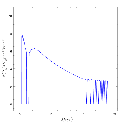
$\nu$ is the efficiency of the star formation process and is set to be $2Gyr^{-1}$ for the Galactic halo ($t<1Gyr$) and $1Gyr^{-1}$ for the disk ($t\geq 1Gyr$). $\Sigma(r,t)$ is the total surface mass density, $\Sigma(r_{\odot},t)$ the total surface mass density at the solar position, $G_{gas}(r,t)$ the surface density normalized to the present time total surface mass density in the disk $\Sigma_{D}(r,t_{Gal})$, where $t_{Gal}=14Gyr$ is the age assumed for the Milky Way and $r_{\odot}=8kpc$ the solar galactocentric distance (Reid 1993). The gas surface exponent, $k$, is set equal to 1.5. With these values for the parameters the observational constraints, in particular in the solar vicinity, are well fitted. Below a critical threshold of the gas surface density ($7M_{\odot}pc^{-2}$) we assume no star formation. This naturally produces a hiatus in the SFR between the halo-thick disk phase and the thin disk phase. In Fig. (1) is shown the predicted star formation rate for the halo-thick disc phase and the thin disc phase, respectively.

Figure 1: The SFR expressed in $M_{\odot}pc^{-2}Gyr^{-1}$ as predicted by the two infall model. The gap in the SFR at the end of the halo-thick disc phase is evident. The oscillations are due to the fact that at the late times in the galactic disc the surface gas density is always close to the threshold density.

For $\phi$, the initial mass function (IMF), we use the Scalo (1986), constant in time and space. $\tau_{m}$ is the evolutionary lifetime of stars as a function of their mass “m”.

The SNeIa rate has been computed following Greggio & Renzini (1983) and Matteucci & Greggio (1986) and it is expressed as:

$$R_{SNeIa}=A\int\limits^{M_{BM}}_{M_{Bm}}\phi(M_{B})(\int\limits^{0.5}_{\mu_{m}}f(\mu)\psi(t-\tau_{M_{2}})d\mu)dM_{B}$$ (3)

where $M_{2}$ is the mass of the secondary, $M_{B}$ is the total mass of the binary system, $\mu=M_{2}/M_{B}$, $\mu_{m}=max\left[M(t)_{2}/M_{B},(M_{B}-0.5M_{BM})/M_{B}\right]$, $M_{Bm}=3M_{\odot}$, $M_{BM}=16M_{\odot}$. The IMF is represented by $\phi(M_{B})$ and refers to the total mass of the binary sistem for the computation of the SNeIa rate, $f(\mu)$ is the distribution function for the mass fraction of the secondary:

$$f(\mu)=2^{1+\gamma}(1+\gamma)\mu^{\gamma}$$ (4)

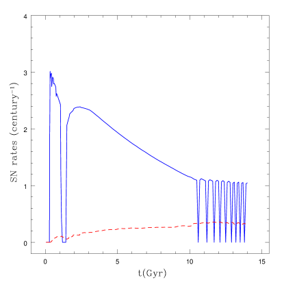
with $\gamma=2$; A is the fraction of systems in the appropriate mass range, which can give rise to SNeIa events. This quantity is fixed to 0.05 by reproducing the observed SNeIa rate at the present time (Cappellaro et al. 1999). Note that in the case of SNIa the“production matrix” is indicated with $Q^{SNIa}_{mi}$ because of its different nucleosynthesis contribution (for details refer to Matteucci and Greggio 1986). In Fig. 2 we show the predicted type II and Ia SN rates. The type II SN rate follows the SFR, as expected, whereas the type Ia SN rate does not have this feature due to the nature of type Ia SN progenitors, which are assumed to be low-intermediate mass star with a long evolutionary time scales.

Figure 2: Predicted SN II (continuous line) and Ia (dashed line) rates by the two infall model.

The last term in equation 1 represents the accretion and it is defined as:

$$A(r,t)=a(r)e^{-t/\tau_{H}}+b(r)e^{(t-t_{max})/\tau_{D}(r)}$$ (5)

$X_{A_{i}}$ are the abundances of infalling material, assumed primordial, $t_{max}=1Gyr$ is the time for the maximum infall rate on the thin disk, $\tau_{H}=2.0Gyr$ is the time scale for the formation of the halo thick-disk and $\tau_{D}$ is the timescale of the thin disk, function of the galactocentric distance:

$$\tau_{D}=1.033r(kpc)-1.267Gyr$$ (6)

The coefficients $a(r)$ and $b(r)$ are constrained by the present day total surface mass density as a function of galactocentric distance. In particular, $b(r)$ is assumed to be different from zero only for $t>t_{max}$, where $t_{max}$ is the time of maximum infall on the thin disc (see Chiappini et al. 2003, for details).

4 Nucleosynthesis Prescriptions

4.1 S-process

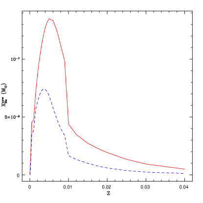
We have adopted the yields of Busso et al. (2001) in the mass range 1.5-3$M_{\odot}$ for the s-main component. In this process, the dependence on the metallicity is very important. In fact, the s-process elements are made by accretion of neutrons on seed elements (in particular iron) already present in the star. Therefore, this Ba component behaves like a secondary element. The neutron flux is due to the reaction ${}^{13}C(\alpha,n)^{16}O$ which can easily be activated at the low temperature of these stars (see Busso et al. 1999). The yields are shown in Table 1 and Fig. 3 as functions of the initial metallicity of the stars. The theoretical results by Busso et al. (2001) suggest negligible Europium production in the s-process and therefore we neglected this component in our work. We have added for models 1 and 2 (see table 2) an extension to the theoretical result of Busso et al. (2001) in the mass range $1-1.5M_{\odot}$ by simply scaling with the mass the values obtained for stars of $1.5M_{\odot}$. We have extended the prescription in order to better fit the data with a [Fe/H] supersolar and it does not change the results of the model at $[Fe/H]<0$.

Table 1: The stellar yields in the range $1.5-3M_{\odot}$ from the paper of Busso et al (2001).

$Metallicity$	$X^{new}_{Ba}$ for $1.5M_{\odot}$	$X^{new}_{Ba}$ for $3M_{\odot}$
0.20$\cdot 10^{-3}$	0.69$\cdot 10^{-8}$	0.13$\cdot 10^{-7}$
0.10$\cdot 10^{-2}$	0.38$\cdot 10^{-7}$	0.46$\cdot 10^{-7}$
0.20$\cdot 10^{-2}$	0.63$\cdot 10^{-7}$	0.87$\cdot 10^{-7}$
0.30$\cdot 10^{-2}$	0.72$\cdot 10^{-7}$	0.11$\cdot 10^{-6}$
0.40$\cdot 10^{-2}$	0.73$\cdot 10^{-7}$	0.12$\cdot 10^{-6}$
0.50$\cdot 10^{-2}$	0.68$\cdot 10^{-7}$	0.13$\cdot 10^{-6}$
0.60$\cdot 10^{-2}$	0.58$\cdot 10^{-7}$	0.13$\cdot 10^{-6}$
0.70$\cdot 10^{-2}$	0.47$\cdot 10^{-7}$	0.12$\cdot 10^{-6}$
0.80$\cdot 10^{-2}$	0.39$\cdot 10^{-7}$	0.11$\cdot 10^{-6}$
0.90$\cdot 10^{-2}$	0.34$\cdot 10^{-7}$	0.98$\cdot 10^{-7}$
0.10$\cdot 10^{-1}$	0.16$\cdot 10^{-7}$	0.43$\cdot 10^{-7}$
0.11$\cdot 10^{-1}$	0.14$\cdot 10^{-7}$	0.39$\cdot 10^{-7}$
0.12$\cdot 10^{-1}$	0.13$\cdot 10^{-7}$	0.34$\cdot 10^{-7}$
0.13$\cdot 10^{-1}$	0.12$\cdot 10^{-7}$	0.32$\cdot 10^{-7}$
0.14$\cdot 10^{-1}$	0.11$\cdot 10^{-7}$	0.29$\cdot 10^{-7}$
0.15$\cdot 10^{-1}$	0.99$\cdot 10^{-8}$	0.27$\cdot 10^{-7}$
0.16$\cdot 10^{-1}$	0.90$\cdot 10^{-8}$	0.25$\cdot 10^{-7}$
0.17$\cdot 10^{-1}$	0.81$\cdot 10^{-8}$	0.23$\cdot 10^{-7}$
0.18$\cdot 10^{-1}$	0.73$\cdot 10^{-8}$	0.22$\cdot 10^{-7}$
0.19$\cdot 10^{-1}$	0.66$\cdot 10^{-8}$	0.20$\cdot 10^{-7}$
0.20$\cdot 10^{-1}$	0.59$\cdot 10^{-8}$	0.19$\cdot 10^{-7}$
0.30$\cdot 10^{-1}$	0.24$\cdot 10^{-8}$	0.94$\cdot 10^{-8}$
0.40$\cdot 10^{-1}$	0.12$\cdot 10^{-8}$	0.50$\cdot 10^{-8}$

Figure 3: The stellar yields $X^{new}_{Ba}$ from the paper of Busso et al (2001) plotted versus metallicity. In dashed line the prescriptions for stars of $1.5M_{\odot}$, in solid line for stars of $3M_{\odot}$.

4.2 R-process

As already said in the introduction the production of r-process elements is still a challenge for astrophysics and even for nuclear physics, due to the fact that the nuclear properties of thousand of nuclei located between the valley of $\beta$ stability and the neutron drip line, necessary to correctly compute this process, are ignored. In our models we have tested 6 different nucleosynthesis prescriptions for the r-process Ba and Eu, as shown in tables 2, 3 and 4. Some of the prescriptions refer to models by Travaglio et al. (2001) (model 3) and Ishimaru et al. (2004)(models 4, 5 and 6), whereas the others contain yields chosen rather “ad hoc”.

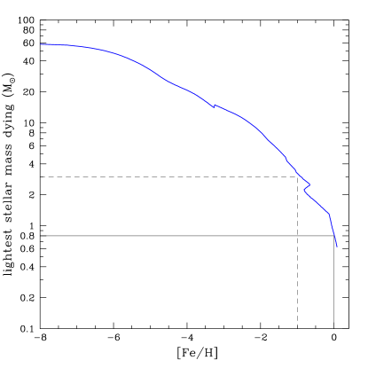
In the case of Ba we have included an r-process component, produced in massive stars in the range 12-30$M_{\odot}$ in model 1 and in the range 10-25$M_{\odot}$ in model 2. In Fig. 4 we show the lightest stellar mass dying as function of the ratio [Fe/H] in our chemical evolution model; it is clear from this plot that it is impossible to explain the observed abundances of [Ba/Fe] in stars with $[Fe/H]<-2$ without the component produced in massive stars. In fact, the first stars, which produce s-processed Ba (see Sect. 4.1), have a mass of $3M_{\odot}$ and they start to enrich the ISM only at $[Fe/H]\geq-2$.

Figure 4: In the plot we show the lightest stellar mass dying at the time corresponding to a given [Fe/H]. The solid line indicates the solar abundance ([Fe/H]=0), corrisponding to a lightest dying mass star of $0.8M_{\odot}$, the dashed line indicates the [Fe/H]=-1 corrisponding to a lightest dying star mass of $3M_{\odot}$.

We stress that Travaglio et al. (2001) predicted r-process Ba only from stars in the range 8-10$M_{\odot}$, but their conclusions were based upon an older set of observational data.

Moreover, we considered another independent indication for the r-process production of Barium; Mazzali and Chugai (1995) observed Ba lines in SN 1987A, which had a progenitor star of 20$M_{\odot}$. These lines of Ba are well reproduced with a overabundance factor $f=X_{obs}/X_{i}=5$ (typical metal abundance for LMC $X_{i}=(1/2.75)\times$ solar). From this observational data we can derive a $X_{Ba}^{new}\sim 2\cdot 10^{-8}$, which is in agreement with our prescriptions.

For the Eu we assumed that it is completely due to the r-process and that the yields originate from massive stars in the range 12-30$M_{\odot}$ in model 1 and 10-25$M_{\odot}$ in model 2, as shown in table 2.

In particular, our choice is done with the purpose of best fitting the plots [Ba/Fe] vs.[Fe/H], [Eu/Fe] vs.[Fe/H] and [Ba/Eu] vs [Fe/H] as well as the Ba and Eu solar abundance (taking in account the contribution of the low-intermediate mass star in case of the Ba).

We have tested prescriptions for Ba and Eu both for a primary production and a secondary production (with a dependence on the metallicity). In the first case the main feature of the yields is a big enhancement in the mass range $12-15M_{\odot}$ (model 1) with no dependence on the metallicity and so the elements are considered as primary elements. In the case of metallicity dependence (model 2), the yield behaviour is chosen to have a strong enhancement in the range of metallicity $5\cdot 10^{-7}<Z<1\cdot 10^{-5}$ with almost constant yield for Eu and Ba in the whole mass range for a given metallicity.

4.3 Iron

For the nucleosynthesis prescriptions of the Fe, we adopted those suggested in François et al. (2004), in particular we considered the yields of Woosley & Weaver (1995) (hereafter WW95) for a solar chemical composition. We remind that the yields suggested for several elements by François et al. (2004) are those reproducing at best the observed [X/Fe] vs. [Fe/H] at all metallicities in the solar vicinity.

Table 2: Model parameters. The yields $X^{new}_{Ba}$ are expressed as mass fractions. The subscript “ext” stands for extended (the yields have been extrapolated down to $1M_{\odot}$) and $M_{*}$ for the mass of the star.

Mod	s-process Ba	r-process Ba	s-process Eu	r-process Eu
1	$1.-3M_{\odot}$	$12-30M_{\odot}$	none	$12-30M_{\odot}$
	Busso et al.(2001)ext.	yields table 3		yields table 3
2	$1.-3M_{\odot}$	$10-25M_{\odot}$	none	$10-25M_{\odot}$
	Busso et al.(2001)ext.	yields table 4		yields table 4
3	$1.5-3M_{\odot}$	$8-10M_{\odot}$	none	$12-30M_{\odot}$
	Busso et al.(2001)	$X^{new}_{Ba}=5.7\cdot 10^{-6}/M_{*}$		yields table 3
		(Travaglio et al. 2001)
4	$1.5-3M_{\odot}$	$10-30M_{\odot}$	none	$8-10M_{\odot}$
	Busso et al.(2001)	yields table 3		$X^{new}_{Eu}=3.1\cdot 10^{-7}/M_{*}$
				(Ishimaru et al.2004 Mod.A)
5	$1.5-3M_{\odot}$	$10-30M_{\odot}$	none	$20-25M_{\odot}$
	Busso et al.(2001)	yields table 3		$X^{new}_{Eu}=1.1\cdot 10^{-6}/M_{*}$
				(Ishimaru et al.2004 Mod.B)
6	$1.5-3M_{\odot}$	$10-30M_{\odot}$	none	$>30M_{\odot}$
	Busso et al.(2001)	yields table 3		$X^{new}_{Eu}=7.8\cdot 10^{-7}/M_{*}$
				(Ishimaru et al.2004 Mod.C)

Table 3: The stellar yields for Barium and Europium in massive stars (r-process) in the case of a primary origin.

$M_{star}$	$X_{Ba}^{new}$	$X_{Eu}^{new}$
12.	9.00$\cdot 10^{-7}$	4.50$\cdot 10^{-8}$
15.	3.00$\cdot 10^{-8}$	3.00$\cdot 10^{-9}$
30.	1.00$\cdot 10^{-9}$	5.00$\cdot 10^{-10}$

Table 4: The stellar yields for Ba and Eu in massive stars (r-process) in the case of secondary origin. The mass fraction does not change in function of the stellar mass.

$Z_{star}$	$X_{Ba}^{new}$	$X_{Eu}^{new}$
	$10-25M_{\odot}$	$10-25M_{\odot}$
$Z<5\cdot 10^{-7}$.	1.00$\cdot 10^{-8}$	5.00$\cdot 10^{-10}$
$5\cdot 10^{-7}<Z<1\cdot 10^{-5}$	1.00$\cdot 10^{-6}$	5.00$\cdot 10^{-8}$
$Z>1\cdot 10^{-5}$	1.60$\cdot 10^{-7}$	8.00$\cdot 10^{-9}$

5 Results

5.1 Trends

In this Sect. we investigate how the different models fit the the trends of the abundances ratios for [Ba/Fe], [Eu/Fe] and [Ba/Eu] versus [Fe/H] and even for [Ba/Eu] versus [Ba/H].

To better investigate the trends of the data we have decided to divide in several bins the [Fe/H] axis and the [Ba/H] axis and compute the mean and the standard deviation from the mean of the ratios [Ba/Fe], [Eu/Fe] and [Ba/Eu] for all the data inside each bin.

In table 5 we show the results of this computation for [Ba/Fe] versus [Fe/H], in table 6 for [Eu/Fe] and [Ba/Eu] versus [Fe/H] and finally in table 7 for [Ba/Eu] versus [Ba/H].

Obviously having the ranges [Ba/H] and [Fe/H] different, we have bins of different width.

We have divided in a different way the [Fe/H] for [Ba/Fe] ratio and the [Fe/H] for [Eu/Fe] and [Ba/Eu] ratios because the [Eu/Fe] ratio for 12 stars at very low metallicity is only an upper limit and therefore the data of these stars have not been considered in the computation of the mean and the standard deviation for [Eu/Fe] and [Ba/Eu] ratios.

In the case of [Ba/Eu] and [Eu/Fe] we have simply divided the [Fe/H] axis in 15 bins of equal dimension (see table 6); for [Ba/Fe] we have divided in 18 bins the [Fe/H] but we have merged the first three bins (starting from the lowest value in [Fe/H]) in a single bin in order to have enough data in the first bin (see table 5). Finally for [Ba/Eu] versus [Ba/H] we have splitted in 16 equal bins but again we have merged the first two pairs in two bins for the same reason (see table 7).

Table 5: Results after the computation of the mean for the data inside bins along the [Fe/H] axis for the values of [Ba/Fe].

bin center [Fe/H]	bin dim.[Fe/H]	mean [Ba/Fe]	SD [Ba/Fe]	N. of data in the bin
-3.82	0.75	-1.25	0.30	6
-3.32	0.25	-0.96	0.50	7
-3.07	0.25	-0.65	0.65	11
-2.82	0.25	-0.37	0.60	17
-2.57	0.25	-0.15	0.40	11
-2.32	0.25	0.09	0.58	13
-2.07	0.25	0.23	0.50	15
-1.82	0.25	0.10	0.20	20
-1.58	0.25	0.08	0.15	27
-1.33	0.25	0.20	0.22	16
-1.08	0.25	0.07	0.19	20
-0.83	0.25	-0.03	0.08	30
-0.58	0.25	-0.04	0.14	59
-0.33	0.25	0.05	0.20	46
-0.08	0.25	0.03	0.13	53
0.17	0.25	-0.01	0.11	26

Table 6: Results after the computation of the mean for the data inside bins along the [Fe/H] axis for the values of [Eu/Fe] and [Ba/Eu].

bin center [Fe/H]	bin dim.[Fe/H]	mean [Eu/Fe]	SD [Eu/Fe]	mean [Ba/Eu]	SD [Ba/Eu]	N of data in the bin
-3.22	0.24	-0.10	0.21	-0.71	0.25	5
-2.98	0.24	0.08	0.60	-0.57	0.13	12
-2.74	0.24	0.46	0.60	-0.64	0.11	14
-2.49	0.24	0.45	0.28	-0.52	0.17	7
-2.25	0.24	0.38	0.36	-0.38	0.33	11
-2.01	0.24	0.51	0.34	-0.36	0.26	10
-1.77	0.24	0.29	0.22	-0.20	0.19	19
-1.53	0.24	0.44	0.15	-0.39	0.22	21
-1.28	0.24	0.42	0.20	-0.26	0.31	18
-1.04	0.24	0.39	0.13	-0.38	0.15	16
-0.80	0.24	0.32	0.12	-0.35	0.14	36
-0.56	0.24	0.23	0.14	-0.27	0.20	55
-0.32	0.24	0.18	0.10	-0.13	0.23	44
-0.07	0.24	0.04	0.07	-0.02	0.14	51
0.17	0.24	-0.02	0.07	0.00	0.12	26

Table 7: Results after the computation of the mean for the data inside bins along the [Ba/H] axis for the values of [Ba/Eu].

bin center [Ba/H]	bin dim.[Ba/H]	mean [Ba/Eu]	SD [Ba/Eu]	N of data in the bin
-4.35	0.58	-0.75	0.26	4
-3.76	0.58	-0.60	0.14	12
-3.32	0.29	-0.55	0.14	3
-3.02	0.29	-0.62	0.13	4
-2.73	0.29	-0.58	0.24	13
-2.43	0.29	-0.58	0.21	4
-2.14	0.29	-0.44	0.13	7
-1.84	0.29	-0.33	0.28	20
-1.54	0.29	-0.33	0.20	25
-1.25	0.29	-0.39	0.19	21
-0.95	0.29	-0.31	0.20	36
-0.66	0.29	-0.33	0.18	64
-0.36	0.29	-0.13	0.14	43
-0.07	0.29	-0.03	0.09	68

Figure 5: In this Fig. is plotted the [Ba/Fe] versus [Fe/H]. The squares are the mean values of the data bins described in the table 5. As error bars we consider the standard deviation (see table 5). The solid line is the results of the model 3 from table 2.

Figure 6: The data are the same as in Fig. 5. In this Fig. we show in solid line the model 1 and in dashed line the model 2 (models are described in table 2) predictions.

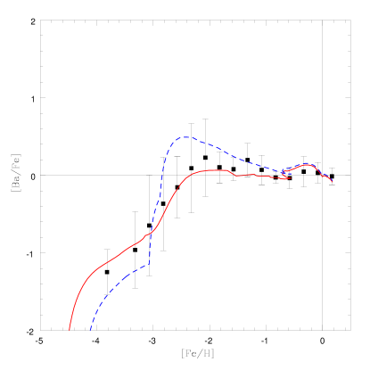
In Fig. 5 we show the results for the model 3 (with the yields used in Travaglio et al. 2001) for [Ba/Fe] versus [Fe/H]. As evident from Fig. 5, this model does not fit the data.

Moreover, the model in Fig. 5 is different from the similar model computed by Travaglio et al. (1999). In fact, we want to underline that we are using a different chemical evolution model and this gives rise to different results. The main difference between the two chemical evolution models (the one of Travaglio and the present one) consists in the age-[Fe/H] relation which grows more slowly in the model of Travaglio. The cause for this difference is probably due to the different adopted stellar lifetimes, to the different $M_{up}$ (i.e. the mass of the most massive star ending its life as C-O white dwarf) and to the yield prescriptions for the iron which are probably the WW95 metallicity dependent ones in the model of Travaglio et al.(1999), whereas we use the WW95 yields for the solar chemical compositios, which produce faster rise of Iron.

In fact, in order to better fit the new data we have to extend the mass range for the production of the r-processed Barium toward higher mass in order to reproduce [Ba/Fe] at lower metallicity.

In Fig. 6, where we have plotted the predictions of the model 1 and the model 2 for [Ba/Fe] versus [Fe/H], it is clear that these models better fit the trend of the data. In these models the upper mass limit for the production of the r-processed Ba is 30$M_{\odot}$ in the case of model 1, and 25$M_{\odot}$ in the case of model 2. However, the model 2 does not fit as well as model 1 the trend of the data but we would like to stress that the prescriptions of model 2 are very simplistic. In fact, there is no dependence on mass for a given metallicity in the yields of Ba and Eu. This prescription is clearly an oversimplification but our goal is to show how a model with yields only dependent on metallicity works and so we are able to better understand at least roughly if it could be a good approach or not.

Figure 7: In graph is plotted the [Eu/Fe] versus [Fe/H]. The squares are the mean values of the data bins described in the table 6. As error bars we consider the standard deviation (see table 6). We show in solid line the results of model 4, in short dashed line the results of model 5 and in long dashed line the ones of model 6 (models are described in table 2)

Figure 8: The data are as in Fig. 7 and in this Fig. we show in solid line the results of the model 1 and in dashed line the results of model 2 (models are described in table 2).

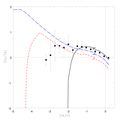
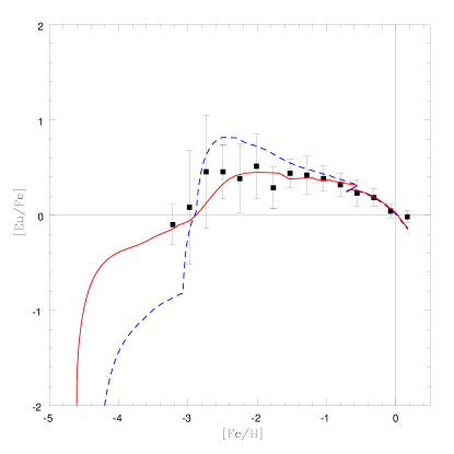
We have obtained similar results comparing the trend of the abundance of [Eu/Fe] versus [Fe/H] with the three models of Ishimaru et al.(2004) (model 4, 5 and 6 in table 2). The chemical evolution of this only r-process element is shown in Fig. 7 and we want to underline again that they used a different chemical model. Again neither model 4 explains the low metallicity abundances nor model 5 and 6 well fit the trend of the data. In Fig. 8 we show the results of the models 1 and 2 in this case for [Eu/Fe] versus [Fe/H]. The trend of the data is well followed by both models from low metallicity to the solar metallicity.

In table 8 we show the predicted solar abundances of Eu and Ba for all our models compared to the solar abundances by Grevesse & Sauval (1998). We have put in the table also the predicted s-process fraction in the Barium solar abundance. The results of almost all our models are in good agreement with the solar abundances with the exception of model 5 which underpredicts the Eu abundance by a factor of nearly 2. Note that we predict a slightly different s-process fraction (nearly 60% instead of 80%) compared with the s-process fraction obtained by previous authors (Travaglio et al. 1999, Arlandini et al. 1999, Raiteri et al. 1992 and Käppeler et al. 1989). This different result is again due to the adopted chemical evolution model, as discussed previously.

Figure 9: In this Fig. we show the ratio of [Ba/Eu] versus [Fe/H]. The squares are the mean values of the data bins described in the table 6. As error bars we consider the standard deviation (see table 6). The results of model 1 are rappresented in solid line, the results of model 2 in long dashed line (models are described in table 2).

Figure 10: In this Fig. we show the ratio [Ba/Eu] versus [Ba/H]. The squares are the mean values of the data bins described in the table 7. As error bars we consider the standard deviation (see table 7). The results of model 1 are rappresente in solid line, the results of model 2 in long dashed line (models are described in table 2).

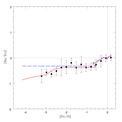
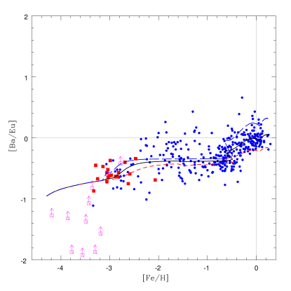
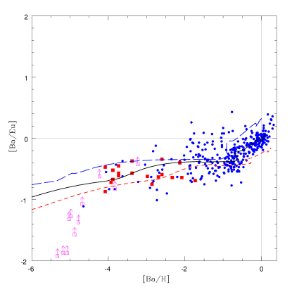
If we look at Fig. 9 where we have plotted the abundances of [Ba/Eu] versus [Fe/H] and at Fig. 10, where is plotted [Ba/Eu] versus [Ba/H], we note three important features. The first is that the spread, that we can infer in these plots from the standard deviation of each bin, is smaller if we use the [Ba/H] ratio in the x axis; the second feature is that it is evident from the data that there is a plateau in the [Ba/Eu] ratio before the production of s-process Ba by the low intermediate mass stars starts to be non negligible at $[Fe/H]\sim-1$ and $[Ba/H]\sim-0.8$; finally, the timescale of rise of the [Ba/Eu] value, due to the production of Ba by low intermediate mass stars, is very well reproduced by our model.

The value of [Ba/Eu] at low metallicity is an important sign to understand the fraction of slow processed Ba in the solar abundance In fact, if the ratio $\frac{Ba_{rapid}}{Eu}$ has a constant value over all the cosmic time, then it must have the same value also at the solar system formation time (if we do not want to add some peculiar effect during the last part of the Galaxy evolution).

In this case the Ba s-process fraction is simply:

$$\frac{Ba_{slow}}{Ba_{total}}=1-10^{[\frac{Ba_{rapid}}{Eu}]}$$

Since we have a mean value for [Ba/Eu] versus [Fe/H] in the range $-3<[Fe/H]<-1$ of -0.44 (taken from the mean value in the bins which fall in that range) and a similar value for [Ba/Eu] versus [Ba/H] in the range $-4<[Ba/H]<-0.8$ of -0.41 (computed in the same way as above), then it turns out that the s-process fraction for Barium slow processed has to be less than the claimed 80% with a value of $\sim 60\%$.

Finally, we want to say that the spread in the ratio of [Ba/Eu] both versus [Fe/H] and [Ba/H] is lower than the spread in [Ba/Fe] and [Eu/Fe], in particular when using as evolutionary tracer the [Ba/H].

In fact, considering the computed standard deviations as spread tracers, where the spread for [Ba/Fe] and [Eu/Fe] is higher ($[Fe/H]\sim-3$), their standard deviations are greater than 0.6 dex whereas the standard deviations for [Ba/Eu] is less than 0.15 dex.

For this reason we believe that the mechanism which produces the observational spread does not affect the ratio of these two elements. In our picture the explanation of the smaller spread in the ratio of [Ba/Eu] is that the site of production of these two elements is the same, the neutronized shell close to the mass cut in a SNII (see Woosley et al. 1994). What changes could be the amount of the neutronized material which each massive star expells during the SNII explosion. In fact, the mass cut and also the ejected neutronized material, are still uncertain quantities and usually they are considered as parameters in the nucleosynthesis codes for massive stars (see Rauscher et al. 2002, Woosley & Weaver 1995, Woosley et al. 1994).

5.2 Comparison with inhomogeneus chemical evolution models

Our chemical evolution model is a model where instantaneous mixing is assumed, (ie. shorter than the timestep of integration of the equations), therefore it is only able to follow the general trends of the abundance ratios as a function of [Fe/H] found in the metal-poor stars. Inhomogeneous models assume that supernovae are able to pollute a small region of gas surrounding them, and depending on the mass of the supernova (hence the yields) and the size of the polluted zone, an abundance spread is predicted. An important point is that the abundance ratios do not change with the amount of gas which is polluted by the supernova. It is therefore interesting to look at the range of the abundance ratios log(Ba/Fe) that we obtain with our model and compare them with the spread found in the observations.

Figure 11: In this Fig we show the ratio between the newly produced Ba and Fe as a function of the stellar mass for the model 1 yields (solid line); the same for Eu in long dashed line.

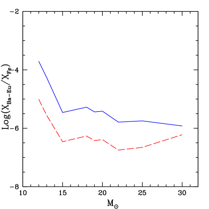
In figure 11 we show the ratio between the r-process elements production and iron production as a function of stellar mass in the range $12-30M_{\odot}$. This means that the maximum spread which could be found with any inhomogeneous model of chemical evolution is shown by the range of abundance ratios displayed in figure 11 i.e. about 2 dex.

The observational data instead are varying in a range which is of the order of 3 dex (see the data in figures 12 for Ba and 13 for Eu). Therefore, even using an inhomogeneous model with our best model yields it would not explain the spread of the data. However, by adjusting the production of Ba and Eu only in a very narrow interval near 10 $M_{\odot}$, one can account for the observed spread. This adjustment may even be justified because SNe of 10 $M_{\odot}$ result in O/Mg/Ne core collapse and make very little Fe, but r-process elements could be produced in the ejecta from the neutron star. A similar approach has been used by the inhomogeneous model of Argast et al. (2004) and by Ishimaru et al. (2004).

From the results obtained in this work, it is not possible to reproduce, even with an inhomogeneous chemical history, such a large spread in the data. It is possible that this discrepancy might be due to the existence of another parameter besides the initial mass determining the SN II yields, such as perhaps the initial angular momentum. In the following section, we explore, under the assumption that the same massive stars contribute both to Fe and r-process synthesis, i.e. without any decoupling, which yield ratios a supernova should produce to explain both the very high and the very low [r-process/Fe] found in the sample of observed halo stars.

5.3 Upper and lower limit to the r-process production

Table 8: Solar abundances of Ba and Eu, as predicted by our models, compared with the observed ones from Grevesse & Sauval (1998).

Mod	$(X_{Ba})_{pr}$	%$Ba_{s}/Ba$	$X_{Ba_{\odot}}$	$(X_{Eu})_{pr}$	$X_{Eu_{\odot}}$
1	$1.55\cdot 10^{-8}$	54%	$1.62\cdot 10^{-8}$	$4.06\cdot 10^{-10}$	$3.84\cdot 10^{-10}$
2	$1.62\cdot 10^{-8}$	51%		$3.96\cdot 10^{-10}$
3	$1.64\cdot 10^{-8}$	44%		As model 1
4	As model 1	As model 1		$4.48.\cdot 10^{-10}$
5	As model 1	As model 1		$1.86\cdot 10^{-10}$
6	As model 1	As model 1		$2.84\cdot 10^{-10}$

The purpose of this Sect. is to give upper and lower limits to the yields in order to reproduce the observed spread at low metallicities for Ba and Eu. We are well aware that an inhomogeneous model would provide better predictions about the dispersion in the [r-process/Fe] ratios if due to yield variations, but we also believe that it is still useful to study the effect of the yield variations by means of our model.

First we explore the range of variations of the yields as functions of the stellar mass. To do this we have worked on the model 1: in particular, we have modified the yields of the model 1 for both elements (Ba and Eu), leaving untouched the s-process yields and changing only the yields of the r-process.

1Max and 1min and their characteristics are summarized in the table 9.

Table 9: The stellar yields for model 1Max and 1Min for Barium and Europium in massive stars (r-process) in the case of a primary origin.

	Model 1Max		Model 1Min
$M_{star}$	$X_{Ba}^{new}$	Factor	$X_{Ba}^{new}$	Factor
12.	1.35$\cdot 10^{-6}$	1.5	4.50$\cdot 10^{-7}$	0.5
$<15$.	4.50$\cdot 10^{-8}$	1.5	1.50$\cdot 10^{-8}$	0.5
$\geq 15$	3.00$\cdot 10^{-7}$	10.	1.50$\cdot 10^{-9}$	0.05
30.	1.00$\cdot 10^{-8}$	10.	5.00$\cdot 10^{-11}$	0.05
$M_{star}$	$X_{Eu}^{new}$	Factor	$X_{Eu}^{new}$	Factor
12.	4.50$\cdot 10^{-8}$	1.	2.25$\cdot 10^{-8}$	0.5
$<15$.	3.00$\cdot 10^{-9}$	1.	1.50$\cdot 10^{-9}$	0.5
$\geq 15$	3.00$\cdot 10^{-8}$	10.	1.50$\cdot 10^{-10}$	0.05
30.	5.00$\cdot 10^{-9}$	10.	2.50$\cdot 10^{-11}$	0.05

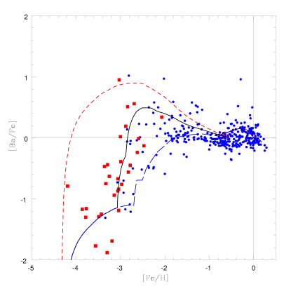
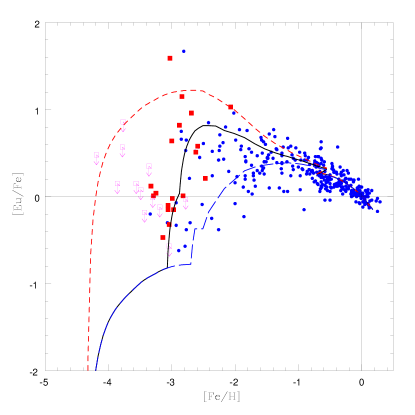
In Fig. 12 and 13 we plot ratios [Ba/Fe] vs [Fe/H] and [Eu/Fe] vs [Fe/H] respectively, for the new models 1Max 1min and 1 compared to the observational data; we show the same plot for the ratios [Ba/Eu] vs [Fe/H] in Fig.14 and and for [Ba/Eu] versus [Ba/H] in Fig. 15.

We can deduce from these upper and lower limit models that the large observed spread could be also due to a different production of heavy elements among massive stars ($>15M_{\odot}$). This type of stars could produce different amounts of these elements independently of the mass. As we have introduced in the previous subsect. (5.1), it is possible to link this fact with the problems of mass cut and the fall back during the explosion of a SNII. If these elements are produced in a shell close to the iron core of the star, differences in the explosion behaviour can give rise to a different quantity of r-process elements expelled by the star.

In this way we are able to explain the presence of the spread for the heavy elements and the absence of the same spread for example in the $\alpha$-elements. In fact, the $\alpha$-elements are produced mostly during the hydrostatic burning of massive stars and then ejected by the explosion.

Figure 12: In this Fig. we show the ratio [Ba/Fe] versus [Fe/H] for the data by François et al. (2005) (filled squares) and for the other observational data (see Sect. 2 in the text, the filled circles). The solid line is the prediction of model 1, the short dashed line the prediction of model 1Max and the long dashed line the prediction of model 1min.

Figure 13: In this Fig. we show the ratio [Eu/Fe] versus the ratio [Fe/H]. The data by François et al. (2005) are with filled squares, wheras the open squares are only upper limits again from the work of François et al. (2005). The filled circles are data by other observational works (see Sect. 2 in the text). The solid line is the prediction of model 1, the short dashed line the prediction of model 1Max and the long dashed line the prediction of model 1min.

Figure 14: In this Fig. we show the ratio [Ba/Eu] versus the ratio [Fe/H]. The data by François et al. (2005) are filled squares, wheras the open squares are only lower limits again from the work of François et al. (2005). The filled circles are data by other observational works (see Sect. 2 in the text). The solid line is the prediction of model 1, the short dashed line the prediction of model 1Max and the long dashed line the prediction of model 1min.

Figure 15: As in Fig. 14 but for the ratio [Ba/Eu] versus [Ba/H].

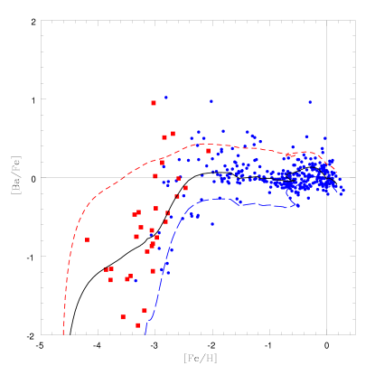
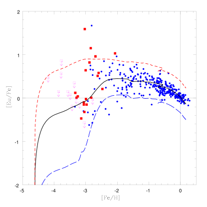
Another approach can be followed to derive again upper and lower limit for the model by changing the yields as functions of metallicity. The model 2, which is the model with yields independent of the mass and depending only on metallicity, will be our test model. In particular, Model 2 assumes for the massive stars different yields for Ba and Eu in three ranges of metallicity (see table 2).

The new prescriptions for both Ba and Eu are summarized in table 10.

Table 10: The stellar yields of model 2Max and model 2min for Ba and Eu in massive stars (r-process).

$Z_{star}$	$Z_{star}$	$X_{Ba}^{new}$	$X_{Eu}^{new}$
model 2Max	model 2min	$10-25M_{\odot}$	$10-25M_{\odot}$
never	$Z<8\cdot 10^{-6}$.	1.00$\cdot 10^{-8}$	5.00$\cdot 10^{-10}$
$Z<1\cdot 10^{-5}$	$8\cdot 10^{-6}<Z<1\cdot 10^{-5}$	1.00$\cdot 10^{-6}$	5.00$\cdot 10^{-8}$
$Z>1\cdot 10^{-5}$	$Z>1\cdot 10^{-5}$	1.60$\cdot 10^{-7}$	8.00$\cdot 10^{-9}$

In Fig. 16 and 17 are shown the results of these two models (2Max and 2min) and of the original model 2 for [Ba/Fe] vs [Fe/H] and for [Eu/Fe] versus [Fe/H] respectively, compared to the observational data.

The results are very interesting. In fact, changing the central range of metallicity, in which there is an enhancement of the production of Ba and Eu, it is possible to produce the upper and the lower limits. These two new models envelope the majority of the data at low metallicities. At higher metallicity the two models overlap the best model and so they do not contain all the spread in this part of the plot but most of them could be explained inside the typical observational error of 0.1 dex.

Figure 16: In this Fig. we show the ratio of [Ba/Fe] versus [Fe/H]. The data are as in Fig. 12. The solid line is the prediction of model 2, the short dashed line the prediction of model 2Max and the long dashed line the prediction of model 2min.

Figure 17: In this Fig. we show the ratio [Eu/Fe] versus the ratio [Fe/H]. The data are as in Fig. 13. The solid line is the prediction of model 2, the short dashed line the prediction of model 2Max and the long dashed line the prediction of model 2min.

6 Conclusions

The main goal of this work was to follow the evolution of Ba and Eu by means of a chemical evolution model well reproducing the abundance trends for other elements. To do that we used the Chiappini et al. (1997) model in its latest version as described in Chiappini et al. (2003). To reach this goal we have used empirical yields for stars with mass $>8M_{\odot}$, producing r-process elements. In fact for the r-process elements there are not solid theoretical yields, since the mechanism which is involved in their production, the so called r-process, is still not well understood. We conclude that Ba needs two components: a s-process main component originating in low mass stars plus a r-component originating in stars in the range 10-30$M_{\odot}$. This range is different from the one suggested by Travaglio et al. (1999) and is obtained by requiring the best fit of the new data. For Eu we estimated that it is mainly produced by an r-process and that stars in the same mass range 10-30$M_{\odot}$ should be considered as the progenitors of this element.

The nearly constant value of the ratio [Ba/Eu] produced in massive stars by the r-process, can be used to estimate the fraction of Barium in the solar abundance produced by the slow process. We have obtained in this way a fraction that is different from the previous results: 60% instead of 80%.

We found that the yields ratios which we obtained to reproduce the trends are not able to explain the large spread found by the observations even with the use of an inhomogeneous model. This implies or the decoupling of the production r-process elements and Fe or a variation of the yields as a function of metallicity for example. It could also that the yields of the r-process are not only a function of the mass of the progenitor.

The yields that we derived and even the fact that the ratio of the r- process production of Eu and Ba seems to be be nearly constant could be very useful to studies involving nucleosynthesis in stellar models and even to nuclear physics studies.

7 Acknowledgments

We thank Francesco Calura and Cristina Chiappini for several useful comments. GC and FM also acknowledge funds from MIUR, COFIN 2003, prot. N. 2003028039.

References

- Argast et al. (2004) Argast D., Samland M., Thielemann F.-K., Qian Y.-Z., 2004 A&A 416, 997
- Arlandini et al. (1999) Arlandini C., Käppeler F., Wisshak K. et al., 1999, ApJ, 525, 886
- Beers et al. (1992) Beers T.C., Preston G.W., Shectman S.A., 1992 A.J., 103, 1987
- Beers et al. (1999) Beers T.C., Rossi S., Norris J.E., Ryan S.G., Shefler T., 1999, A.J., 117, 981
- Burris et al. (2000) Burris D.L., Pilachowski, C.A., Armandroff T.E. et al., 2000, ApJ, 544, 302
- Busso et al (2001) Busso M., Gallino R., Lambert D.L., Travaglio, C., Smith V.V., 2001, ApJ, 557, 802
- Busso et al. (1999) Busso M., Gallino R.,Wasserburg G.J., 1999 ARA&A ,37, 239
- Cappellaro et al. (1999) Cappellaro E., Evans R., Turatto M., 1999, A&A, 351, 459
- Cayrel et al. (2004) Cayrel R., Depagne E.,Spite M. et al., 2004, A&A, 416, 1117
- Chiappini et al. (1997) Chiappini C., Matteucci M.F., Gratton R.G., 1997, ApJ, 477, 765
- Chiappini et al. (2003) Chiappini C., Romano D., Matteucci M.F., 2003, MNRAS, 339, 63
- Clayton & Rassbach (1967) Clayton D.D., Rassbach, M.E., 1967, ApJ, 168, 69
- François et al. (2005) François P., Depagne E., Hill V. et al., 2005, in preparation
- François et al. (2004) François P., Matteucci F., Cayrel R. et al., 2004, A&A, 421, 613
- Freiburghaus et al. (1999) Freiburghaus C., Rosswog S., Thielemann F.-K., 1999, ApJ, 525L, 121
- Fulbright (2000) Fulbright J.P., 2000, AJ, 120, 1841
- Gallino et al. (1998) Gallino R., Arlandini C., Busso M. et al., 1998, ApJ, 497, 388
- Greggio & Renzini (1983) Greggio L., Renzini A., 1983, A&A, 118, 217
- Grevesse & Sauval (1998) Grevesse N., Sauval A.J., 1998, Space Sci. Rev., 85, 161
- Honda et al. (2004) Honda S., Aoki W., Kajino T. et al., 2004, ApJ, 607, 474
- Ishimaru & Wanajo (1999) Ishimaru Y., Wanajo S., 1999,ApJ, 511L, 33
- Ishimaru et al. (2004) Ishimaru Y., Wanajo S.,Aoki, W., Ryan, S.G., 2004,ApJ, 600L, 47
- Käppeler et al. (1989) Käppeler F., Beer H., Wisshak K., 1989, Rep.Prog.Phys., 52, 945
- Kennicutt (1989) Kennicutt R.C.Jr., 1989, ApJ, 344, 685
- Kennicutt (1998) Kennicutt R.C.Jr., 1998, ApJ, 498, 541
- Koch & Edvardsson (2002) Koch A., Edvardsson B., 2002, A&A,381, 500
- Martin & Kennicutt (2001) Martin C.L., Kennicutt R.C.Jr., 2001, ApJ, 555, 301
- Mathews et al (1992) Mathews, G. J., Bazan, G., Cowan, J. J., 1992, ApJ, 391, 719
- Matteucci &François (1989) Matteucci M.F., François P., 1989, MNRAS, 239, 885
- Matteucci & Greggio (1986) Matteucci M.F., Greggio L., 1986, A&A, 154, 279
- Mashonkina & Geheren (2000) Mashonkina L., Gehren T., 2000, A&A, 364, 249
- Mashonkina & Geheren (2001) Mashonkina L., Gehren T., 2001, A&A , 376, 232
- Mazzali & Chugai (1995) Mazzali, P. A., Chugai, N. N., 1995, A&A, 303, 118
- McWilliam et al. (1995) McWilliam A., Preston G.W., Sneden C., Searle L., 1995, AJ, 109, 2757
- Pagel & Tautvaisienne (1995) Pagel B.E.J., Tautvaisienne G., 1995 MNRAS, 276, 505
- Pagel & Tautvaisienne (1997) Pagel B.E.J., Tautvaisienne G., 1997 MNRAS, 288, 108
- Raiteri et al. (1992) Raiteri C.M., Gallino R., Busso M., 1992, ApJ, 387, 263
- Raiteri et al. (1993) Raiteri C.M., Gallino R., Busso M., 1993, ApJ, 419, 207
- Rauscher et al. (2002) Rauscher T., Heger A., Hoffmann R.D., Woosley S.E., 2002, ApJ, 576, 323
- Reid (1993) Reid M.J., 1993, ARAA, 31, 345
- Ryan et al. (1996) Ryan S., Norris J.E., Beers T.C., 1996, ApJ, 471, 254
- Scalo (1986) Scalo J.M., 1986, FCPh, 11, 1
- Travaglio et al. (1999) Travaglio C., Galli D., Gallino R. et al., 1999, ApJ, 521, 691
- Travaglio et al. (2001) Travaglio C., Galli D., Burkert A., 2001, ApJ, 547, 217
- Tsujimoto et al. (1999) Tsujimoto T., Shigeyama T., Yoshii Y., 1999, ApJ, 519L, 63
- Wanajo et al. (2003) Wanajo S., Tamamura M., Itoh N. et al., 2003, ApJ, 593, 968
- Woosley & Hoffmann (1992) Woosley S.E., Hoffmann, R.D., 1992, ApJ, 395, 202
- Woosley & Weaver. (1995) Woosley S.E., Weaver, T.A., 1995, ApJ, 101, 181
- Woosley et al. (1994) Woosley S.E., Wilson J.R., Mathews G.J., Hoffman R.D., Meyer B.S., 1994, ApJ, 433, 229