Modelling galaxy spectra in presence of interstellar dust.
I. The model of ISM and the library of dusty SSPs

Abstract

The advent of modern infrared astronomy has brought into evidence the role played by the interstellar dust in galaxy formation and evolution. Therefore, to fully exploit modern data, realistic spectrophotometric models of galaxies must include this important component of the interstellar medium (ISM).

In this paper, the first of a series of two devoted to modelling the spectra of galaxies of different morphological type in presence of dust, we present our description of the dust both in the diffuse ISM and the molecular clouds (MCs).

Our galaxy model contains three interacting components: the diffuse ISM, made of gas and dust, the large complexes of MCs in which active star formation occurs and, finally, the populations of stars that are no longer embedded in the dusty environment of their parental MCs.

Our model for the dust takes into account three components, i.e. graphite, silicates and polycyclic aromatic hydrocarbons (PAHs). We consider and adapt to our aims two prescriptions for the size distribution of the dust grains and two models for the emission of the dusty ISM. We cross-check the emission and extinction models of the ISM by calculating the extinction curves and the emission for the typical environments of the Milky Way (MW) and the Large and Small Magellanic Clouds (LMC and SMC) and by comparing the results with the observational data. The final model we have adopted is an hybrid one which stems from combining the analysis of Guhathakurta & Draine (1989) for the emission of graphite and silicates and Puget et al. (1985) for the PAH emission, and using the distribution law of Weingartner & Draine (2001a) and the ionization model for PAHs of Weingartner & Draine (2001b).

We apply the model to calculate the spectral energy distribution (SED) of Single Stellar Populations (SSPs) of different age and chemical composition, which may be severely affected by dust at least in two types of star: the young, massive stars while they are still embedded in their parental MCs and the intermediate- and low-mass AGB stars when they form their own dust shell around (see Piovan et al., 2003, for more details about AGB stars).

We use the ”Ray Tracing” method to solve the problem of radiative transfer and to calculate extended libraries of SSP SEDs. Particular care is paid to model the contribution from PAHs, introducing different abundances of $C$ in the population of very small carbonaceous grains (VSGs) and different ionization states in PAHs. The SEDs of young SSPs are then compared with observational data of star forming regions of four local galaxies successfully reproducing their SEDs from the UV-optical regions to the mid and far infrared (MIR and FIR, respectively).

Galaxy spectra with interstellar dust

1 Introduction

The interstellar dust, either tightly associated to stars and/or dispersed in the ISM, has got more and more attention over the years, in particular with the advent of modern infrared satellites (e.g. IRAS, COBE and ISO), because of its role in many astrophysical phenomena (see Draine, 2003a, b, c, 2004, for more details).

Leaving exceptions aside, there are at least three main circumstances in which dust influences the stellar light: (i) It is long known that for a certain fraction of their life very young stars are embedded in the parental MCs. Even if the duration of this obscured period is short, its effect on the light emitted by these stars cannot be neglected as a significant fraction of the light (initially almost all) is shifted to the IR region of the spectrum. (ii) Low and intermediate mass stars in the Asymptotic Giant Branch (AGB) phase may form an outer dust-rich shell of material obscuring and reprocessing the radiation emitted by the star underneath. (iii) Finally, thanks to the contribution of metal-rich material by supernovae and stellar winds in Wolf-Rayet and AGB stars, the ISM acquires over the years a dust rich component. The UV-optical radiation emitted by stars passing through this dust-rich intergalactic gas is absorbed and then re-emitted in the far IR.

In this paper, first we develop a model for the absortiom/emission properties of a dusty medium and second we apply it to derive the SED of young stars still embedded in their parental MCs. In a companion paper (Piovan et al., 2005), we will present detailed chemo-spectrophotometric models of galaxies of different morphological type whose SED from the UV to the far IR is derived including dusty MCs and the presence of diffuse, dust-rich ISM.

Stars are preferentially born inside massive, dense and cool MCs characterized by low temperatures $\left(T\lesssim 9-15\textrm{K}\right)$, masses in the range from $\sim 10^{4}$ to $10^{6}M_{\odot}$ and dimensions from $\sim 6$ to $60pc$, the most massive and big ones being less numerous (Solomon et al., 1987). Furthermore all regions with active star formation, e.g. in the MW, are also associated to $H_{2}$ clouds, thanks to which the MCs are mapped by means of radio surveys. In general they seem to be organized in hierarchical structures forming very complicate and large complexes, inside which a large number of substructures of higher density are found. The observation of the earliest evolutionary phases of young stars is severely hampered by the presence of dust, which absorbs and diffuses a large fraction of the radiation emitted by the stars in the optical returning it in the MIR/FIR. However, as soon as the first-born, massive stars evolve, their strong stellar winds and mass-loss, intense ionizing radiation fields and final explosion as type II supernovae will eventually destroy the MCs in which they are embedded. Massive stars become eventually visible in UV-optical regions of the spectrum. The time scale for this to occur is $\sim 10^{6}-10^{8}$ years, i.e. the lifetime of the most massive stars in the population. To summarize, we are able to map the location of MCs thanks to radio data, to follow the first evolutionary stages of star formation thanks to FIR data and finally to directly observe the stars in the UV-optical when the parental clouds have been evaporated. However all intermediate stages are precluded to direct observations because they are obscured by dust. They must be inferred from theory, which unfortunately is still far from being fully satisfactory.

The problem is particularly severe when the evolutionary population synthesis technique (EPS) is applied to model the SED, the integrated magnitudes and broad-band colors of galaxies, by folding the properties of SSPs of different age and chemical composition on the star formation history (SFH). Classical studies of this subject (Bruzual & Charlot, 1993; Bressan et al., 1994; Tantalo et al., 1996, 1998; Fioc & Rocca-Volmerange, 1997; Chiosi et al., 1998) ignore the presence of dust on the light emitted by SSPs. In other words, ”bare” spectra of SSPs are used to synthesize the SED of a galaxy. This approximation sounds acceptable when modelling the SED of old systems, such as early-type galaxies, in which star formation took place long ago, even if also in this case the presence of dust around AGB stars should not be ignored (Piovan et al., 2003; Temi et al., 2004). This is certainly not the case with the late-type and starburst galaxies that are rich of gas, dust and stars of any age. Therefore, it is mandatory to include the effect of dust on the radiation emitted by young stars. Because of the high density in the regions of star formation, the optical depth may be very high also for IR photons and the full problem of radiative transfer has to be considered.

The plan of the paper is as follows. In Sect. 2 we model in detail the extinction and emission properties of the dusty ISM. In particular we present the optical properties of graphite, silicates and PAHs, the two distribution laws for the grain sizes (shortly named MRN ad WEI models), the cross sections and the dust to gas ratio. In Sect. 3 we address the topic of emission from dust grains, and present two models shortly indicated as GDP and LID. The theory is applied to derive the average extinction curves and emission properties for the diffuse ISM of the MW, LMC and SMC (Sects. 4, 4.1, and 4.2, respectively). Then we apply our best solution for the ISM extinction and emission to derive the SEDs of young dusty SSPs. We summarize the fundamentals of spectral synthesis in Sect. 5 and in Sect. 6 we present our choice for the spatial distribution of young stars inside the MCs. In Sect. 7 we cast the problem of radiative transfer introducing the key parameters and discussing the dependence of the optical depth on the cloud physical parameters. In addition to this, we quickly summarize the the ”ray tracing” technique to solve the problem of radiative transfer throughout an absorbing/emitting medium. In Sect. 8 we present the SEDs of very young SSPs surrounded by their MCs. Having in mind the application of our results to studies of population synthesis in galaxies (Piovan et al., 2005), we have calculated a library of young SEDs with dust for large ranges of the parameters, paying particular attention to the emission of PAHs. In addition to this, we show results for a simple way of modelling the evaporation of the MCs surrounding young SSPs. In Sect. 9 we compare our SEDs with observational data of star forming regions. To this aim, we considered the central regions of four starburst galaxies, namely Arp$220$, NGC$253$, M$82$ and NGC$1808$. Finally, in Sect. 10 we draw some general remarks and conclusions.

2 Modelling the properties of dust

Chief workbenches for the study of the physical properties of the interstellar grains are the extinction curves and the IR emission of dust observed with growing detail in different physical environments. From the characteristic broad bump of the extinction curves in the UV at $2175$ Å  and the absorption features at $9.7\mu m$ and $18\mu m$ (Draine, 2003c) we can already infer that a two components model made of graphite and silicates is required. The study of the emission adds further constraints. A population of VSGs has been invoked to reproduce the emissions observed by IRAS in the pass-bands $12\mu m$ and $25\mu m$. The VSGs temperatures can fluctuate well above $20\ \textrm{K}$ if their energy content is small compared to the energy of the absorbed photons (Leger & Puget, 1984; Desert et al., 1986; Dwek, 1986; Guhathakurta & Draine, 1989; Siebenmorgen & Kruegel, 1992; Draine & Li, 2001; Li & Draine, 2001). Excluding that VSGs are made of silicates simply because the $10\mu m$ emission feature of silicates is not detected in diffuse clouds (Mattila et al., 1996; Onaka et al., 1996), most likely they are made of carbonaceous material with broad ranges of shapes, dimensions, and chemical structures (see also Desert et al., 1986; Li & Draine, 2002a, for a discussion of this topic).

Emission lines at $3.3$, $6.2$, $7.7$, $8.6$, and $11.3\mu m$, originally named unidentified infrared bands (UIBs), have been firstly observed in luminous reflection nebulae, planetary HII regions and nebulae (Sellgren et al., 1983; Mathis, 1990) and subsequently also in the diffuse ISM with IRTS (Onaka et al., 1996; Tanaka et al., 1996) and ISO (Mattila et al., 1996). There is nowadays the general consensus that these lines owe their origin to the presence of PAH molecules, vibrationally excited by the absorption of a UV-optical photon (Leger & Puget, 1984; Li & Draine, 2001). Currently these spectral features are commonly referred to as the aromatic IR bands (AIBs).

Based on these considerations, any realistic model of a dusty ISM, to be able to explain the UV-optical extinction and the IR emission of galaxies, has to include at least three components, i.e. graphite, silicates, and PAHs. Furthermore, while it may treat the big grains as in thermal equilibrium with the radiation field, it has to allow the VSGs to have temperatures above the mean equilibrium value. In order to obtain the properties of a mixture of grains, we have to specify their cross sections, their dimensions, and the kind of interaction with the local radiation field.

Optical properties. The optical properties of PAHs, silicate and graphite grains together with the corresponding dimensionless scattering and absorption coefficients, $Q_{sca}(a,\lambda)$ and $Q_{abs}(a,\lambda)$ have been taken from Draine & Lee (1984), Laor & Draine (1993), Draine & Li (2001) and Li & Draine (2001). These coefficients are defined as the ratio of the cross section $\sigma$ to the geometrical section $\pi a^{2}$, where $a$ is the dimension of the grain.

Distribution laws: MRN-like and WEI models. In the ISM the grain dimensions are likely to vary over a large range of values. Therefore in order to properly model the optical properties of the ISM we need to specify the distribution law of the grain dimensions and to fix their upper and lower limits. Two cases are considered.

In the first one, shortly referred to as ”WEI”, we adopt the analytical law proposed by Weingartner & Draine (2001a). It is a very complicate relationship for the size distribution of carbonaceous dust grains, which simultaneously deals with graphite and PAHs and smoothly shifts from PAHs to small graphite grains, considering PAHs as the extension of carbonaceous grains down to the molecular regime:

$$\frac{1}{n_{H}}\frac{dn_{g}}{da} = D\left(a\right)+\frac{C_{g}}{a}\left(\frac{a}{a_{t,g}}\right)^{\alpha_{g}}F\left(a,\beta_{g},a_{t,g}\right)\times$$ (3)

$$\times \negmedspace\left\{\begin{array}[]{ll}1\qquad\qquad\qquad\qquad\hskip 8.53581pt3.5\textrm{\AA}<a<a_{t,g}\\ exp\left\{-\left[\left(a-a_{t,g}\right)/a_{c,g}\right]^{3}\right\}\quad\hskip 2.84526pta>a_{t,g}\\ \end{array}\right.$$

where $C_{g}$ is the abundance of carbon, $a_{t,g}$ is a transition radius securing a smooth cut-off for dimensions $a>a_{t,g}$, $a_{c,g}$ is a parameter that controls the cut-off steepness, and $\alpha_{g}$ is the exponent of the power law. $D\left(a\right)$, the sum of two log-normal terms that helps to better reproduce the emission by very small carbonaceous grains, is given by

$$\frac{1}{n_{H}}\left(\frac{dn_{g}}{da}\right)_{vsg} = D\left(a\right)$$ (4)

$$= \sum_{i=1}^{2}\frac{B_{i}}{a}\exp\left\{-\frac{1}{2}\left[\frac{\ln\left(a/a_{0,i}\right)}{\sigma}\right]^{2}\right\}$$

for $a>3.5$ Å. Following Weingartner & Draine (2001a), the term $B_{i}$ is

$$B_{i} = \frac{3}{\left(2\pi\right)^{3/2}}\frac{\exp\left(-4.5\ \sigma^{2}\right)}{\rho a_{0,i}^{3}\sigma}$$ (5)

$$\times \frac{b_{C,i}m_{C}}{1+erf\left[3\sigma\sqrt{2}+\ln\left(a_{0,i}/3.5\AA\ \right)/\sigma\sqrt{2}\right]}$$

where $m_{C}$ is the mass of a C atom, $\rho=2.24g\ cm^{-3}$ is the density of graphite, $b_{C,1}=0.75\ b_{C}$, $b_{C,2}=0.25\ b_{C}$ with $b_{C}$ the total C abundance (per H nucleus) in the log-normal populations, $a_{0,1}=3.5$ Å, $a_{0,2}=30$ Å and $\sigma=0.4$. The function $F\left(a,\beta_{g},a_{t,g}\right)$ in eqn. 3 is a suitable correcting term of curvature [see eqn. (6) in Weingartner & Draine (2001a) for more details]. Finally, to obtain the total abundance of carbon we need to add the contributions coming from the two log-normal distributions, i.e. $D\left(a\right)$, to the term controlled by $C_{g}$. An interesting property of eqn. (3) is that thanks to its ad-hoc analytical form very good fits of the extinction curves are possible by varying the contribution of the very small carbonaceous grains to the $C$ abundance in the ISM, a quantity not yet firmly assessed. As shown by Weingartner & Draine (2001a), the sole extinction curve cannot constrain the carbon abundance $b_{C}$, but only provide an upper limit. For any ratio of visual extinction to reddening $R_{V}=A\left(V\right)/E\left(B-V\right)$, the limit is reached when the very small carbonaceous grains (PAHs and small graphite grains) are able to account for all the ultraviolet bump of the extinction curve. A relationship similar to eqn. (3) is adopted in Weingartner & Draine (2001a) for the silicate grains but, since there is no need for log-normal distributions of VSGs, the abundance of silicates is completely described by the parameter $C_{s}$. With the aid of the above relations by Weingartner & Draine (2001a) it is possible to reproduce the average extinction curves of the diffuse and dense ISM of the MW, LMC and SMC.

In the second case, shortly referred to as ”MRN”, we have modified and extended the power-law proposed by Mathis et al. (1977). To better explore all the possible situations, we split the distribution law of the i-th component in several intervals labelled by $k$

$$\frac{1}{n_{H}}\frac{dn_{i}}{da}=\left\{\begin{array}[]{ll}A_{i}a^{\beta+\beta_{1}}a_{b_{1}}^{-\beta_{1}},&a_{c_{1}}<a<a_{c_{2}}\\ A_{i}a^{\beta+\beta_{2}}a_{b_{2}}^{-\beta_{2}},&a_{c_{2}}<a<a_{c_{3}}\\ ....................,&.....................\\ A_{i}a^{\beta+\beta_{k-1}}a_{b_{k-1}}^{-\beta_{k-1}},&a_{c_{k-1}}<a<a_{c_{k}}\\ \end{array}\right.$$ (6)

with the condition that $a^{\beta+\beta_{j}}a_{b_{j}}^{-\beta_{j}}\approx a^{\beta+\beta_{j+1}}a_{b_{j+1}}^{-\beta_{j+1}}$ where $j=1,...,k-2$ if $k>2$. The meaning of $a_{c_{k}}$ is obvious, whereas the $a_{b_{k}}$ are the ”modulation factors” introduced by Draine & Anderson (1985). For $k=2$ relation (6) reduces to a single power-law distribution with $a_{c_{1}}=a_{min}$ and $a_{c_{k}}=a_{max}$. Usually, $k=2$ for PAHs, and $2\leq k\leq 4$ for silicates and carbonaceous grains. In most cases we adopt $k=2$ or $k=3$. More complicated power laws are obtained with $k=4$.

Cross sections The cross sections of scattering, absorption and extinction for the grain mixture in each component of the ISM are defined as

$$\sigma_{p,i}\left(\lambda\right)=\int_{a_{\min,i}}^{a_{\max,i}}\pi a^{2}Q_{p,i}\left(a,\lambda\right)\frac{1}{n_{H}}\frac{dn_{i}(a)}{da}da$$ (7)

where the index $p$ stands for absorption (abs), scattering (sca), total extinction (ext) and the index $i$ identifies the type of grains, $a_{min,i}$ and $a_{max,i}$ are the lower and upper limits of the size distribution for the i-type of grain, and finally $n_{H}$ is the number density of $H$ atoms. The total dimension-less extinction coefficient is $Q_{ext}\left(a,\lambda\right)=Q_{abs}\left(a,\lambda\right)+Q_{sca}\left(a,\lambda\right)$.

With the aid of the above cross sections it is possible to calculate the optical depth $\tau_{p}(\lambda)$ along a given path

$$\tau_{p}\left(\lambda\right)=\sum_{i}\sigma_{p,i}\left(\lambda\right)\int_{L}n_{H}dl=\sum_{i}\sigma_{p,i}\left(\lambda\right)\times N_{H}$$ (8)

where $L$ is the optical path and the meaning of the other symbols is the same as before. In this expression for the various $\tau_{p}(\lambda)$ we have implicitly assumed that the cross sections remain constant along the optical path.

Dust to gas ratio The coefficients $b_{C}$, $C_{g}$, $C_{s}$ for the WEI model and $A_{i}$ for the MRN model fix the abundances of carbon and silicates with respect to the abundance of hydrogen. In order to apply our models to a wide range of metallicities and ages, it is important to discuss how these coefficients would change as function of the chemical composition of the ISM (the metallicity at least). The dust-to-gas ratio is defined as $\delta=M_{d}/M_{H}$ where $M_{d}$ and $M_{H}$ are the total dust and hydrogen mass, respectively. If $m_{i}$ is the total mass of the $i$-th type of grains then $M_{d}=\sum_{i}m_{i}$, where the mass $m_{i}$ is obtained from integrating over the grain size distribution (which depends also on the abundance coefficients). Knowing the gas content of a galaxy (in principle function of the age), the amount of dust in the ISM depends on $\delta$. For the MW and other galaxies of the Local Group, $\delta$ is estimated to vary from $1/100$ to $1/500$. In models for the MW, $\delta=0.01$ is often adopted, while $\delta=0.00288$ and $\delta=0.00184$ are typical values for the LMC and SMC. The mass-density ratios of interstellar dust are roughly in the proportion $1:1/3:1/5$ going from the MW to the LMC and SMC (Pei, 1992). A simple way of incorporating the effect of metallicity is to assume that $\delta\varpropto Z$ in such a way to match the approximate average results for MW, LMC and SMC: $\delta=\delta_{\odot}\left(Z/Z_{\odot}\right)$. This relation simply implies that metal-rich galaxies are also dust-rich. The above relation $\delta\varpropto Z$ agrees with the results by Dwek (1998) based on evolutionary models for the compositions and abundances of gas and dust in the MW. However, it oversimplifies the real situation.

The slope of the extinction curves greatly varies passing from the MW to LMC and SMC. Moreover, the bump due to graphite decreases from MW to LMC and SMC (Calzetti et al., 1994). These differences have been attributed to the metallicity decreasing from $Z=Z_{\odot}$ in the solar vicinity, to $Z=\frac{1}{3}Z_{\odot}$ in the LMC, and $Z=\frac{1}{5}Z_{\odot}$ in the SMC. However, the metallicity difference does not only imply a difference in the absolute abundance of heavy elements in the dust, but also a difference in the relative proportions, i.e. in the composition pattern. Probably the ratio graphite to silicates varies from galaxy to galaxy. Despite these uncertainties (Devriendt et al., 1999), the relation $\delta\varpropto Z$ is adopted to evaluate the amount of dust in galaxy models (e.g. Silva et al., 1998) by simply scaling the dust content adopted for the ISM of the MW to the metallicity under consideration. In this study, using the data for the extinction curves and emission of the MW, LMC and SMC, we seek to build a model of the dusty ISM describing the effect of different metallicities in a more realistic way. It is clear, however, that the problem remains unsettled for metallicities higher than the solar one, for which we have no information. The relation $\delta\varpropto Z$ together with the relative proportions holding good for the MW extinction curve, can be reasonably adopted also for other dusty ISMs characterized by metallicities close to the one of the MW.

3 Emission models

In the following, two cases are considered to evaluate the emission of a dusty ISM. First, the easy to calculate model that stems from the thermal-continuous approach by Guhathakurta & Draine (1989) for the temperature fluctuations of silicate and graphite grains and a modification of the prescriptions by Puget et al. (1985) for the temperature fluctuations of PAHs. The calculation of the ionization state of PAHs is also properly introduced following Weingartner & Draine (2001a). We will refer to it as the ”GDP” model. Second, a more elaborated model in which we implement the state-of-the art for the temperature fluctuations of the very small grains as recently proposed by Draine & Li (2001) and Li & Draine (2001). This model will be shortly indicated as the ”LID” model.

3.1 The GDP model

Emission from silicate and graphite grains. In order to calculate the temperature distribution acquired by small spherical grains of dust heated by photons and collisions with energetic particles, it is useful to define a vector state $P\left(t\right)$. The state of a grain is determined by its enthalpy $E$ and the components $P_{k}\left(t\right)$ of the state vector are the probability for a grain to find itself in the $k$-th bin of enthalpy at the time $t$. The enthalpy spans the range $\left[E_{\min},E_{\max}\right]$ which in turn splits into $N$ discrete bins each of which characterized by $E_{k}$ and $\Delta E_{k}$, i.e. the average value of the enthalpy and the width of the enthalpy bin. The enthalpy grid we have adopted is the same as in Guhathakurta & Draine (1989).

Let us also define the transition matrix $A_{f,i}$ representing the probability for unit time that a grain in the state $i$ may undergo a transition to the state $f\neq i$. Neglecting the transitions to enthalpies outside the interval $\left[E_{\min},E_{\max}\right]$, the condition of statistical equilibrium (steady state) is given by $dP_{f}^{ss}/dt=0$ (Guhathakurta & Draine, 1989; Draine & Li, 2001). Taking into account all the transitions to and from any bin we have $\sum\limits_{i=1}^{N}A_{f,i}P_{i}^{ss}=0$. Together with the normalization $\sum_{i=1}^{N}P_{i}^{ss}=1$ condition, it forms a system of linear equations whose solution yields the equilibrium temperature distribution. All technical details on the solution of this steady state system and the transition matrix $A_{f,i}$ can be found in Guhathakurta & Draine (1989) and Draine & Li (2001).

The enthalpy and temperature intervals are usually chosen in such a way that the distribution function $P_{k}\left(T\right)$ smoothly changes from one bin to another and the energy balance between absorption and emission is conserved. Lis & Leung (1991) use a grid with $N\simeq 200$. However Siebenmorgen & Kruegel (1992) note that grids with high $N$ do not necessarily improve the accuracy of $P_{k}\left(T\right)/\Delta E_{k}$ and accordingly adopt $N\simeq 60$, even if $N\simeq 30$ could be sufficient in some cases. In the latest models of Draine & Li (2001) the number $N$ of bins is in the range $300<N<1500$, each bin (the first ones in particular) contains at least two vibrational states, the bin widths smoothly vary and the last bin is chosen at high enough energy so that the expected population is very small (probability $P_{N}<10^{-14}$). Here we adopt $N\simeq 150-200$, which seems to secure computational speed and accuracy at the same time.

A question soon arises: below which dimensions $a_{flu}$ must the temperature fluctuations be taken into account? According to Guhathakurta & Draine (1989) and Siebenmorgen & Kruegel (1992), the typical dimension separating small from large grains is about $a_{flu}\simeq 150$Å  independently of the radiation field. However, this conclusion was questioned by Li & Draine (2001) who found that also for dimensions of the order of $a_{flu}\simeq 200$Å the temperature distribution is sufficiently broad thus introducing some uncertainty in the estimate of the emission. To take this remark into account we adopt here $a_{flu}\simeq 250$Å. Finally, the emission $j_{\lambda}^{small}$ for small graphite and silicate grains is given by

$$j_{\lambda}^{small} = \pi\int\nolimits_{a_{min}}^{a_{flu}}\int\nolimits_{T_{min}}^{T_{max}}a^{2}Q_{abs}\left(a,\lambda\right)B_{\lambda}\left(T\left(a\right)\right)\times$$ (9)

$$\times\frac{dP\left(a\right)}{dT}dT\frac{1}{n_{H}}\frac{dn\left(a\right)}{da}da$$

where $dP\left(a\right)/dT$ is the distribution temperature obtained for the generic dimension $a$, and $B_{\lambda}\left(T\left(a\right)\right)$ is the Planck function.

In the case of grains with dimensions larger than about $\sim 250\textrm{\AA}$ which remain cool because of their high thermal capacity and re-emit the energy absorbed from the incident radiation field into the FIR, a good approximation is to evaluate the equilibrium temperature $T\left(a\right)$ from the balance between absorption and emission

$$\int Q_{abs}\left(a,\lambda\right)J_{\lambda}d\lambda=\int Q_{abs}\left(a,\lambda\right)B_{\lambda}\left(T\left(a\right)\right)d\lambda$$ (10)

where $J_{\lambda}$ is the incident radiation field. With the aid of $T\left(a\right)$ we calculate the emission assuming that big grains of fixed composition and radius behave like a black body. Therefore, the emission coefficient is

$$j_{\lambda}^{big}=\pi\int_{a_{flu}}^{a_{max}}a^{2}Q_{abs}\left(a,\lambda\right)B_{\lambda}\left(T\left(a\right)\right)\frac{1}{n_{H}}\frac{dn\left(a\right)}{da}da$$ (11)

Emission from PAHs. Let us consider a photon of energy $E=h\nu^{{}^{\prime}}=hc/\lambda^{{}^{\prime}}$ impinging on a PAH molecule. The maximum temperature increase caused by the absorption of the photon is given by the solution of the equation

$$\frac{hc}{\lambda^{{}^{\prime}}}=\int\nolimits_{T_{min}}^{T_{max}\left(\lambda^{{}^{\prime}},a\right)}C_{PAH}\left(T,a\right)dT$$ (12)

where $T_{min}\thicksim 5\ \textrm{K}$ and $C_{PAH}\left(T,a\right)$ is the thermal capacity of a grain of dimension $a$ at the temperature $T$. As pointed out by Xu & de Zotti (1989), $T_{max}(\lambda^{{}^{\prime}},a)$ is essentially independent from the choice of $T_{min}$. In order to calculate $C_{PAH}\left(T,a\right)$, we use the numerical fit of the Léger et al. (1989) relationship proposed by Silva et al. (1998):

$$\frac{C_{PAH}\left(T,a\right)}{C_{max}}=\left\{\begin{array}[]{llll}mT&&&T\leq 800\ \textrm{K}\\ nT+p&&&800\ \textrm{K}\leq T\leq 2100\ \textrm{K}\\ 1&&&T\geq 2100\ \textrm{K}\end{array}\right.$$ (13)

where $m=9.25\cdot 10^{-4}$, $n=2\cdot 10^{-4}$, $p=0.58$, and $C_{max}=3\left[\left(N_{C}+N_{H}\right)-2\right]k_{B}$ (Léger et al., 1989). $N_{C}$ and $N_{H}$ are the number of hydrogen and carbon atoms in the molecule, and $k_{B}$ is the Boltzmann constant.

Dealing with the number $N_{H}$ of H atoms in a PAH an important issue has to be clarified. The PAHs in the ISM are subject to many physical and chemical processes, chief among which are the ionization and photo-dissociation caused by the absorption of a UV photon, electron recombination with PAH cations, and chemical reactions between PAHs and other major elemental species in the ISM.

PAHs can be dehydrogenated (some of the $C-H$ bonds can be broken), fully hydrogenated (one H atom for every available C site) or highly hydrogenated (some of the peripheral $C$ atoms bear two $H$ atoms). The reason is that $H$ atoms are less strongly bound ($4.5eV$) than carbon atoms ($7.2eV$) and therefore can be more easily removed by energetic photons (Leger et al., 1989).

Over the years many studies have been devoted to model the hydrogenation state at various levels of sophistication (Allain et al., 1996a, b; Vuong & Foing, 2000) and recently Le Page et al. (2001) and Le Page et al. (2003) presented a very detailed model for the charge and hydrogenation state of PAHs. The number of $H$ atoms is given by the relation $N_{H}=\chi_{H}\cdot N_{S}$ where $N_{S}$ is the number of available sites for hydrogen to bind to carbon and $\chi_{H}$ is the hydrogenation factor. In a PAH with full hydrogen coverage, the bond between $N_{S}$ and $N_{H}$ depends on nesting the hexagonal cycles into the molecule. These cycles can form (i) an elongated low-density object, named catacondensed PAH (linear chains of n-cycles with general scheme $C_{4n+2}H_{2n+4}$, like naphthalene with 2 cycles, anthracene with 3 cycles, and pentacene with 5 cycles); (ii) a compact object named pericondensed PAH described by the formula $C_{6p^{2}}H_{6p}$, like coronene with $p=2$, ovalene and circumcoronene or (iii) an untied object (biphenile). The more compact the PAH, the more stable it is.

In agreement with this, to represent the main characteristics of the interstellar PAHs, Omont (1986), Dartois & D’Hendecourt (1997) and Li & Draine (2001) consider models of pericondensed PAHs, coronene-like, that are more stable against photodissociation by UV photons.

From the formula for compact pericondensed PAHs with full hydrogen coverage, $C_{6p^{2}}H_{6p}$, we get $N_{S}=6p=\left(6\cdot 6p^{2}\right)^{0.5}=\left(6N_{C}\right)^{0.5}$. As the number $N_{C}$ of carbon atoms is known, we can derive the number $N_{S}$ of sites available for bonds. For example, for the coronene with $p=2$ and $N_{C}=24$, we have $N_{S}=12$; if the coverage is full with $\chi_{H}=1$, we have $N_{H}=12$. We are left with the hydrogenation $\chi_{H}$ factor to be determined. This will depend on the ISM conditions. For typical astronomical environments, Siebenmorgen & Kruegel (1992) have suggested dehydrogenated values from $0.01$ to $0.5$, without excluding values as low as $0.01$. More recent studies by Le Page et al. (2001) and Le Page et al. (2003) adopt hydrogenation factors that depend on the PAH dimensions. Their analysis splits the population of PAHs in several groups. At the typical conditions of the diffuse ISM, their general conclusion is that very small PAHs (those with less than $30$ $C$ atoms) are extremely dehydrogenated, larger PAHs with more than $30$ $C$ atoms have full hydrogen coverage, whereas very large PAHs (with more than 150-200 $C$ atoms) can be highly hydrogenated. As the model proposed by Le Page et al. (2001) and Le Page et al. (2003) is too much detailed for the purposes of this study, the $H/C$ ratios in usage here are taken from Li & Draine (2001)

$$H/C=\left\{\begin{array}[]{ll}0.5&\quad N_{C}\leq 25\\ 0.5/\sqrt{N_{C}/25}&\quad 25\leq N_{C}\leq 100\\ 0.25&\quad N_{C}\geq 100\end{array}\right.$$ (14)

They yield $N_{H}=N_{S}=\left(6N_{C}\right)^{0.5}$ in the range $25\leq N_{C}\leq 100$, which is typical of a pericondensed PAH with full hydrogen coverage, while only for smaller PAHs there is a partial dehydrogenation.

To calculate the emission of the PAHs we start defining the power irradiated by a molecule of dimension $a$ at the temperature $T$

$$F\left(T,a\right)=\int_{0}^{\infty}\pi a^{2}Q_{abs}^{PAH}\left(a,\lambda\right)\pi B\left(\lambda,T\right)d\lambda$$ (15)

where $B\left(\lambda,T\right)$ is the Planck function. Once heated to a temperature $T$, the molecule cools down at the rate

$$\frac{dT}{dt}=\frac{F\left(T,a\right)}{C_{P}\left(T,a\right)}$$ (16)

The energy emitted at the wavelength $\lambda$ by a PAH of dimension $a$, as a consequence of absorbing a single photon with energy $hc/\lambda^{{}^{\prime}}$, is given by

$$S = \int\nolimits_{0}^{t}\pi a^{2}Q_{abs}^{PAH}\left(a,\lambda\right)\pi B\left(\lambda,T\right)dt=$$ (17)

$$= \int\nolimits_{T_{min}}^{T_{max}}\pi a^{2}Q_{abs}^{PAH}\left(a,\lambda\right)\pi B\left(\lambda,T\right)\frac{C_{P}\left(T,a\right)}{F\left(T,a\right)}dT$$

where $S=S(\lambda^{{}^{\prime}},\lambda,a)$ and $T_{max}=T_{max}(\lambda^{{}^{\prime}},a)$.

Under the effect of an incident radiation field $I(\lambda^{{}^{\prime}})$ containing photons of any energy, the emission at the wavelength $\lambda$ per $H$ atom becomes

$$J\left(\lambda\right) = \frac{1}{n_{H}}\int\nolimits_{a_{PAH}^{low}}^{a_{PAH}^{high}}\frac{dn_{PAH}\left(a\right)}{da}\pi a^{2}Q_{abs}^{PAH}\left(a,\lambda\right)\times$$ (18)

$$\times\int\nolimits_{0}^{\infty}\frac{I(\lambda^{{}^{\prime}})}{hc}\lambda^{{}^{\prime}}\pi a^{2}Q_{abs}^{PAH}\left(a,\lambda^{{}^{\prime}}\right)\times$$

$$\times\int\nolimits_{T_{min}}^{T_{max}}\pi B\left(\lambda,T\right)\frac{C_{P}\left(T,a\right)}{F\left(T,a\right)}dT\,d\lambda^{{}^{\prime}}\,da$$

from which

$$J\left(\lambda\right) = \frac{\pi}{n_{H}hc}\int\nolimits_{\lambda_{MIN}}^{\lambda_{MAX}}I\left(\lambda^{{}^{\prime}}\right)\lambda^{{}^{\prime}}\int\nolimits_{a_{PAH}^{low}}^{a_{PAH}^{high}}\frac{dn_{PAH}\left(a\right)}{da}$$ (19)

$$a^{2}Q_{abs}^{PAH}\left(a,\lambda^{{}^{\prime}}\right)S\left(\lambda^{{}^{\prime}},\lambda,a\right)da\,d\lambda^{{}^{\prime}}$$

The many types of PAHs can differ not only for the hydrogen coverage on peripheral carbon atoms, but also for the ionization state. Because of their low ionization potential (about $6-7\ eV$), on one hand the PAHs can be ionized by photo-electric effect (Bakes & Tielens, 1994), on the other hand they can also acquire charge through collisions with ions and electrons (Draine & Sutin, 1987). Consequently, there is always some probability that a PAH is in a charged state. Therefore, Li & Draine (2001) have calculated and made available PAHs cross sections both for ionized and neutral PAHs. Since the ionization state will affect the intensity of AIBs, as we can see in Fig. 1, in our calculations we have included the ionization of PAHs.

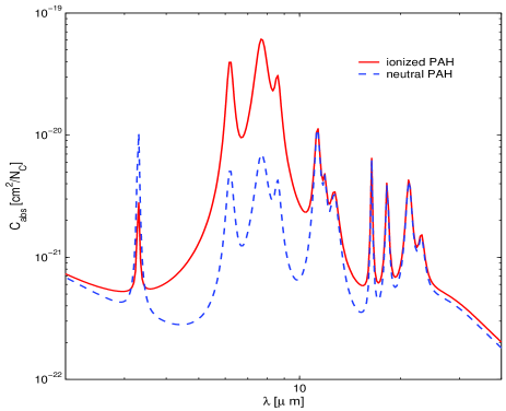
Figure 1: Optical properties of neutral and ionized PAHs containing $40$ atoms of carbon in the IR spectral region of the UIBs. The difference between neutral (dashed line) and ionized PAHs is soon evident: the ionization enhances the stretching modes C-C ($6,2$ and $7.7\,\mu m$) and the bending mode C-H ($8.6\mu m$), whereas it weakens the stretching mode C-H at $3.3\,\mu m$ (Li & Draine, 2001).

To this aim, the charge-state distribution model of PAHs is taken from Weingartner & Draine (2001b), who improved upon previous attempts by Draine & Sutin (1987) and Bakes & Tielens (1994). Indicating with $Z$ the charge state of a PAH molecule, in conditions of statistical equilibrium we have the following relation

$$f\left(Z\right)\left[J_{pe}\left(Z\right)+J_{ion}\left(Z\right)\right]=f\left(Z+1\right)J_{e}\left(Z+1\right)$$ (20)

where $f\left(Z\right)$ is the probability for a PAH to possess the charge $Z$ (either positive or negative), $J_{pe}$ is the photo-emission rate, $J_{ion}$ is the positive ion accretion rate, and finally $J_{e}$ is the electron accretion rate. Following Draine & Sutin (1987), $f\left(Z\right)$ is derived by recursively applying eqn. (20) to $f\left(0\right)$. We obtain

$$f\left(Z\right)=f\left(0\right)\prod_{Z^{\prime}=1}^{Z}\left[\frac{J_{pe}\left(Z^{\prime}-1\right)+J_{ion}\left(Z^{\prime}-1\right)}{J_{e}\left(Z^{\prime}\right)}\right]$$ (21)

for $Z>0$, whereas for $Z<0$ we have

$$f\left(Z\right)=f\left(0\right)\prod_{Z^{\prime}=Z}^{-1}\left[\frac{J_{e}\left(Z^{\prime}+1\right)}{J_{pe}\left(Z^{\prime}\right)+J_{ion}\left(Z^{\prime}\right)}\right]$$ (22)

The constant $f\left(0\right)$ is derived from the normalization condition

$$\sum^{\infty}_{-\infty}f\left(Z\right)=1$$ (23)

The expressions for $J_{pe}$, $J_{ion}$ and $J_{e}$ are taken from Weingartner & Draine (2001b). As both neutral and ionized PAHs are present, we indicate with $\chi_{i}=\chi_{i}\left(a\right)$ the fraction of ionized PAHs of dimension $a$, and with $Q_{abs}^{IPAH}$ and $Q_{abs}^{NPAH}$ the absorption coefficients of ionized and neutral PAHs. Including both types of PAHs into eqn. (19) we obtain

$$J\left(\lambda\right) = \frac{\pi}{n_{H}hc}\int\nolimits_{\lambda_{min}}^{\lambda_{max}}I\left(\lambda^{{}^{\prime}}\right)\lambda^{{}^{\prime}}\int\nolimits_{a_{PAH}^{low}}^{a_{PAH}^{high}}\frac{dn_{PAH}\left(a\right)}{da}\times$$

$$\times a^{2}\left[Q_{abs}^{IPAH}\left(a,\lambda^{{}^{\prime}}\right)S_{ION}\left(\lambda^{{}^{\prime}},\lambda,a\right)\chi_{i}+\right.$$

$$+ \left.Q_{abs}^{NPAH}\left(a,\lambda^{{}^{\prime}}\right)S_{NEU}\left(\lambda^{{}^{\prime}},\lambda,a\right)\left(1-\chi_{i}\right)\right]dad\lambda^{{}^{\prime}}$$

3.2 The LID model

We have also implemented in our code the physical and numerical treatment of the infrared emission of the ISM developed by Draine & Li (2001) and Li & Draine (2001), which is currently considered as the state-of-the art of the subject and has already been used by Li & Draine (2002b) to study the IR emission of the SMC. Owing to its complexity, we will limit ourselves to mention here only a few basic aspects of the model. For all details the reader should refer to Draine & Li (2001) and Li & Draine (2001, 2002b). In this model, made of three components, i.e. graphite, silicates and PAHs, the energy and temperature increase of the dust grains caused by the absorption of energetic photons is calculated by means of the density states of vibrational energy levels. The task is accomplished in three possible ways: the exact statistical method, the thermal discrete approximation and the thermal continuous approach. The latter two make use of the same energy bins of the exact statistical approximation, but differ in the way the transitions to higher (by absorption) and/or lower levels (by emission) are treated. Among the many improvements upon thermal models made in the past, we call particular attention on (i) the detailed calculation of vibrational modes using the harmonic oscillator approximation, (ii) the much better estimate of the probability of grains to be in the fundamental state and (iii) the relationship between vibrational energy and ”temperature” of the grains. We have considered here both types of thermal model, leaving the exact statistical treatment aside because the enormous computational time required makes it difficult to implement it in spectrophotometric models of galaxies. In Fig. 2 we show the energy distribution functions of the silicates for the thermal discrete model under the effect of the Mathis et al. (1983) radiation field. It is worth noticing how the probability for the small grains to be in the ground state is high, even if the distribution extends to high energy states. This accurate description of the ground state can not be obtained with the GDP model.

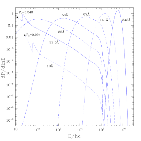
Figure 2: The energy distribution functions of silicate grains with dimensions of $10$Å, $22.5$Å, $35$Å, $56$Å, $89$Å, $141$Å, $242$Å as indicated. All the distributions have been calculated using the thermal discrete model of Draine & Li (2001). Following Li & Draine (2001), we mark with a filled circle the first excited state. $P_{0}$ is the probability for the grains to be in the ground state that for small dimensions is high even if the distribution extends to high energy states.

4 Extinction and emission in the MW, LMC and SMC

As first step toward including dust emission and extinction in the SED of young SSPs and galaxies with different shapes, different histories of star formation and chemical enrichment, different contents of gas, dust and metals at the present time, we seek to reproduce the average extinction curves of the MW, LMC and SMC and to match the emission of their dusty diffuse ISM. As the MW, LMC and SMC constitute a sequence of decreasing mean metallicity, they provide the ideal workbench to calibrate the model for the ISM as a function of the metal content. Although including the effect of systematic differences in the metal content is of paramount importance, this aspect is not always fully taken into account. For instance Silva et al. (1998) adopt for the diffuse ISM with different chemical compositions a model originally designed for the MW, and include the effect of different metallicities by simply scaling the abundance of dust with the metallicity (see also Devriendt et al., 1999, for more details).

The procedure we have adopted iteratively tries to simultaneously satisfy the constraints set by emission and extinction until self-consistency is achieved. It is also worth mentioning here that our approach somehow improves upon the analysis by Takagi et al. (2003), who did not test their dust model on the IR emission of the SMC. Unfortunately, we cannot test the model predictions for the emission of PAHs in the LMC because no data are available (see also Takagi et al., 2003). Nevertheless, making use of COBE and IRAS data, and coupling the fits of the emission and extinction curves we can put some constraints on the flux intensity and the relative weight of the dust components.

We present results obtained with the various models to our disposal, i.e. the GDP and LID model for emission and the WEI and our MRN-like distribution for the grain sizes. By comparing results from each possible combination we look for the one best suited to model the SED of SSPs and galaxies.

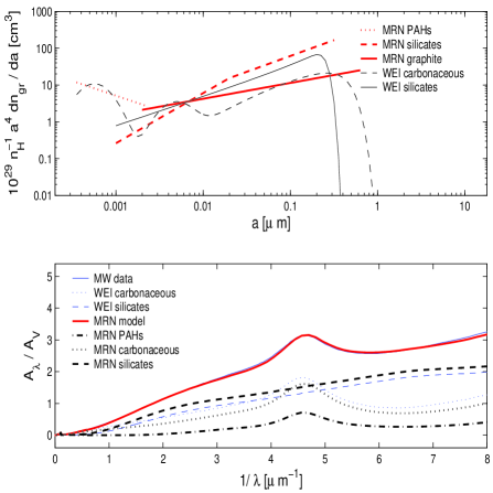
Figure 3: Top Panel: The normalized distribution laws (number density as a function of dimensions) for different types of grain. For the MRN model we show the graphite grains (thick continuous line), silicate grains (thick dashed line) and PAHs (thick dotted line). For the WEI model we display the carbonaceous grains (thin dashed line) and silicate grains (thin continuous line). Bottom Panel: The extinction curve for the diffuse ISM of the MW obtained with a mixture made of graphite, silicates and PAHs. In this panel several cases are shown. First of all the total extinction for our MRN-like model (thick solid line) and for the WEI model (thin solid line) together with the observational data (same thin solid line). All the three lines are practically coincident. In addition to this for each case we show the contribution from the different types of grains: the silicates for the MRN and WEI models are indicated with the thick dashed and the thin dashed lines, respectively; the contribution of graphite in the MRN model and of carbonaceous grains in the WEI model are displayed by thick dotted and thin dotted lines, respectively; finally, for MRN model the contribution of PAHs is shown by the thick dot-dashed line.

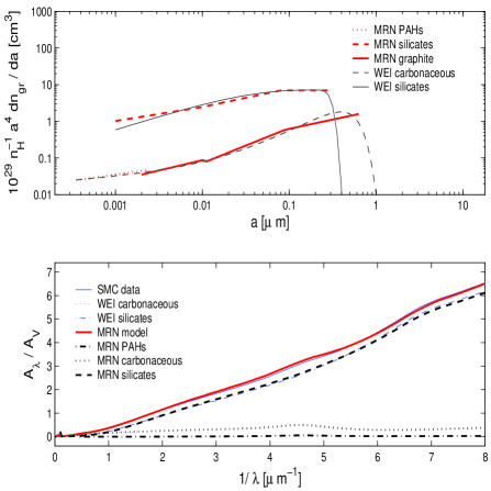
Figure 4: The same as in Fig. 3 but for the SMC. The data for the extinction curve of the SMC along the line of sight of the star AzV398 are taken from Gordon & Clayton (1998).

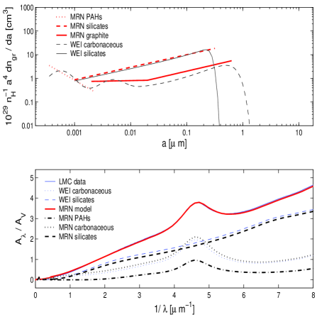
Figure 5: The same as in Figs. 3 and 4 but for the LMC. The data for the extinction curve of the LMC are from Misselt et al. (1999).

4.1 The extinction curves of the MW, LMC and SMC

The best fit of the extinction curves for the three galaxies under examination is derived from minimizing the $\chi$-square error function for which we adopt the Weingartner & Draine (2001a) definition

$$\chi^{2}=\sum_{i=1}^{n}\frac{\left(\frac{A_{obs}\left(\lambda_{i}\right)}{A_{obs}\left(V\right)}-\frac{A_{mod}\left(\lambda_{i}\right)}{A_{mod}\left(V\right)}\right)^{2}}{\sigma_{i}^{2}}$$ (25)

where $A_{obs}\left(\lambda_{i}\right)/A_{obs}\left(V\right)$ represent the observational data normalized to the V band, $A_{mod}\left(\lambda_{i}\right)/A_{mod}\left(V\right)$ are the values of the model, and $\sigma_{i}$ are the weights (Weingartner & Draine, 2001a). Typically the number of test-points $n$ is of the order of $100$. We use as optimization technique the Levenberg-Marquardt method (see Press et al., 1992, for more details) combined with a sampling algorithm in bounded hypercubes and some manual pivoting of the parameters. In any case, it is worth noticing that the problem is very complicate because the multi-dimensional solution space is characterized by many local minima to which the solution may converge missing the true minimum.

In Table (1), we list the parameters we have found from the best-fit of the extinction curves of the MW, LMC, and SMC, respectively, using the MRN model. The WEI model is also shown for comparison.

The MRN-like distribution given by eqn. (6) has been used with $n=2$ or $n=3$ for graphite and silicates and $n=2$ for PAHs for the MW and LMC, whereas for the SMC a more complicated relationship has been adopted. Some parameters are kept fixed for all the models: i.e. the lower limits for the size distribution of PAHs and silicates which are set at the lowest values for which the cross sections are available, $3.5$Å and $10$Å, respectively, and the upper limit of the silicates and graphite distribution fixed at $0.3\,\mu m$ and about $1\,\mu m$. An important parameter is the upper limit of the PAH distribution, which is coincident with the lower limit of the graphite distribution: the two populations do not overlap and the PAHs are considered as the small-size tail of the carbonaceous grains. The transition size has been fixed at $20$Å thus allowing both PAHs and small, thermally fluctuating, graphite grains to concur to shape the SED in the MIR. The exact value of the transition size has in practice no influence on the extinction curve thanks to the similar UV-optical properties of PAHs and small graphite grains. The same considerations do not clearly apply to the IR emission, where a large population of PAHs will produce stronger emission in the UIBs. On the contrary, in Weingartner & Draine (2001a) and Li & Draine (2001), PAHs and graphite grains are included in the family of the so called ”carbonaceous grains”, where the smallest grains have the PAHs optical properties, the biggest grains have the graphite properties, and for the intermediate dimensions a smooth transition from PAHs to graphite properties is adopted.

Table 1: Best fit parameters for the extinction curve of the diffuse ISM of the MW with $R_{V}=3.1$, for the average extinction curve of the LMC and for the flat extinction curve of the SMC. For MW graphite and PAHs we adopt $k=2$, whereas for silicates we use $k=3$. For LMC silicates and PAHs we adopt $k=2$, whereas for graphite we use $k=3$. Finally, in the case of SMC, for PAHs we adopt $k=2$, whereas for graphite we use $k=4$ because we need a more complex set of power-law distributions.

		MW			LMC			SMC
	Graphite	Silicates	PAHs	Graphite	Silicates	PAHs	Graphite	Silicates	PAHs
$A$	$-25.79$	$-25.19$	$-25.18$	$-25.96$	$-25.35$	$-25.26$	$-26.68$	$-25.58$	$-26.73$
$\beta$	$-3.57$	$-3.54$	$-3.5$	$-3.5$	$-3.47$	$-3.37$	$-3.495$	$-3.5$	$-3.48$
$\beta_{1}$	–	$0.9$	$-1.3$	$-0.5$	–	$-2$	$0.058$	$-0.117$	$-0.18$
$\beta_{2}$	–	$0.4$	–	–	–	–	–	$-0.5$	–
$\beta_{3}$	–	–	–	–	–	–	–	–	–
$a_{c_{1}}$	$2\cdot 10^{-7}$	$1\cdot 10^{-7}$	$3.5\cdot 10^{-8}$	$2\cdot 10^{-7}$	$1\cdot 10^{-7}$	$3.5\cdot 10^{-8}$	$2\cdot 10^{-7}$	$1\cdot 10^{-7}$	$3.5\cdot 10^{-8}$
$a_{c_{2}}$	$1\cdot 10^{-4}$	$2\cdot 10^{-6}$	$2\cdot 10^{-7}$	$2\cdot 10^{-6}$	$3\cdot 10^{-5}$	$2\cdot 10^{-7}$	$1\cdot 10^{-6}$	$1\cdot 10^{-6}$	$2\cdot 10^{-7}$
$a_{c_{3}}$	–	$3\cdot 10^{-5}$	–	$1\cdot 10^{-4}$	–	–	$9\cdot 10^{-6}$	$8\cdot 10^{-6}$	–
$a_{c_{4}}$	–	–	–	–	–	–	$1.05\cdot 10^{-4}$	$3\cdot 10^{-5}$	–
$a_{b_{1}}$	–	$2\cdot 10^{-6}$	–	$2\cdot 10^{-6}$	–	$2\cdot 10^{-7}$	–	$1\cdot 10^{-6}$	$3.5\cdot 10^{-8}$
$a_{b_{2}}$	–	$2\cdot 10^{-6}$	–	–	–	–	$9\cdot 10^{-6}$	$8\cdot 10^{-6}$	–
$a_{b_{3}}$	–	–	–	–	–	–	–	–	–

¹All the dimensions are in cm.

The final results for the extinction models, are shown in Figs. 3, 4, and 5 for the MW, SMC and LMC, respectively. The top panels show the scaled abundances of the various components in both the MRN- and WEI-models, i.e. PAHs, graphite and silicates in the former, carbonaceous and silicates in the latter. The bottom panels show the corresponding extinction curves, first separately for each component, then the total for both the MRN- and WEI-models, and finally the observational data. The MRN- and WEI-models coincide and both are nearly indistinguishable from the observational data. Furthermore, it is worth noticing that in order to obtain good fits for the MW, LMC and SMC the grain size distributions need to be more complicate than the simple power law by Mathis et al. (1977). Both in MRN- and WEI- models, the number of free parameters is about $10$. If a single power-law is adopted as in Mathis et al. (1977) to reduce the number of parameters, we fail to get a good fit for all the three extinction curves. The worst situation is with the SMC. The absence of the bump in the extinction curve makes it difficult to get a good fit without increasing the number of adjustable parameters. The missing bump is indeed a strong constraint. Finally, our MRN-model best solution tends to yield abundances and overall results in close agreement with those by Weingartner & Draine (2001a).

4.2 Emission by the diffuse ISM of MW, LMC and SMC

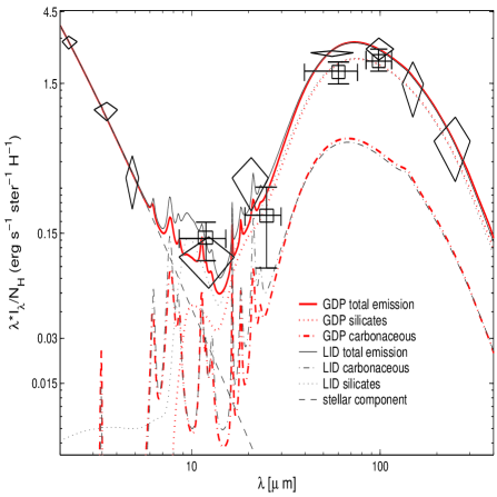
Figure 6: Emission of the diffuse ISM predicted by models containing graphite, silicates and PAHs and comparison with the observational data for the SMC Bar. The thick lines show the GDP emission model coupled with our MRN-like grain distribution for SMC. The thin lines display the thermal discrete LID emission model of Li & Draine (2001) and Draine & Li (2001) coupled with the WEI distribution for SMC (Weingartner & Draine, 2001a). The separate contributions from different grains are also shown: the solid lines are the total emission; the dotted lines are the emission of silicates; the dot-dashed line are the ones of carbonaceous grains; finally the contribution of the stellar component is indicated by the dashed line. The incident radiation field is the standard MMP (Li & Draine, 2002b). The data from COBE/DIRBE (diamonds) and IRAS (squares) have been kindly provided by Li (2004, private communication). See also Li & Draine (2002b).

Matched the extinction curves, we also need to test the overall consistency of the model as far as the IR emission by dust and the comparison with the observational data for the SMC and MW are concerned. For LMC no data are available and the Li & Draine (2001) model is taken as reference model.

The two models of emission (GDP and LID) presented in Sects. 3.1 and 3.2 must be coupled with the two models for the grain distribution (MRN and WEI) both of which fairly reproduce the extinction curves as amply discussed in Sect. 4.1.

The combination of WEI distribution with the LID model would be the ideal case to deal with (Li & Draine, 2001; Draine & Li, 2001). However, we limit ourselves to consider only the cases GDP+MRN and GDP+WEI, because the GDP model is much faster than LID and therefore more suited to spectrophotometric synthesis. The LID model will be, however, considered as the reference case for comparison. The guide-line here is to cross check results for extinction and emission and by iterating the procedure to contrive the parameters at work so that not only unrealistic solutions are ruled out (that could originate by sole fit of the extinction curve) but also additional information on the overall problem is acquired.

The preliminary step to undertake is to choose the radiation field heating up the grains. We adopt the Mathis et al. (1983) interstellar radiation field (MMP) for the solar neighborhood of the MW, both for the whole MW and the LMC, whereas a slightly different radiation field is adopted for the SMC Bar. As this region presents a large spread in radiation intensities, following Li & Draine (2002b) and Dale et al. (2001), the intensity of the radiation impinging on the dust grains has been described with a power-law distribution $dN_{H}/dU$ of MMP radiation fields (Li & Draine, 2002b).

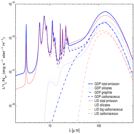
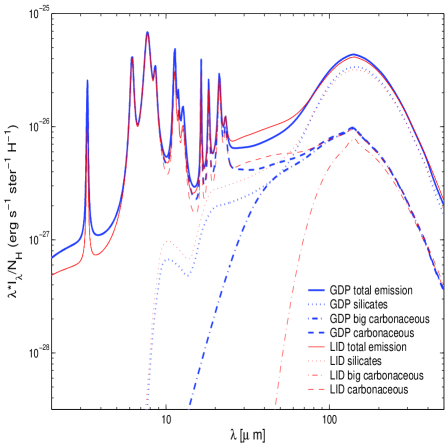
Figure 7: Left Panel: Emission of the diffuse ISM predicted by models containing graphite, silicates and PAHs appropriate to the case of the LMC. The thick lines correspond to the GDP emission model with our prescription for MRN-like distribution law suited to the LMC. The thin lines are the thermal discrete LID emission model of Li & Draine (2001) and Draine & Li (2001) with the WEI distribution law (Weingartner & Draine, 2001a). The separate contributions from different grains are also shown: the solid lines are the total emission; the dotted lines are the emission of silicates; the dot-dashed lines are the ones of graphite grains; finally, the short dashed lines are the total emission of carbonaceous grains, graphite plus PAHs. The incident radiation field is the standard MMP. Right Panel: the same as in the Left Panel but in all cases the distribution law of Weingartner & Draine (2001a) is adopted.

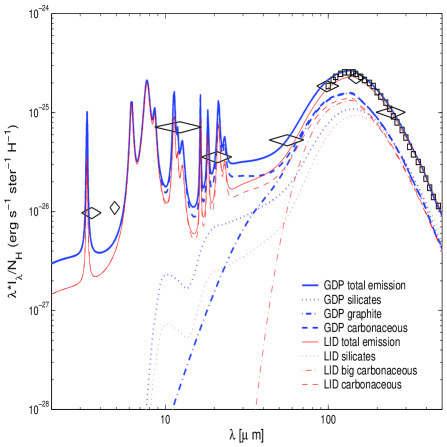
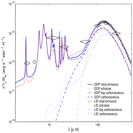
Figure 8: Left Panel: Emission of the diffuse ISM in the MW towards high Galactic latitudes $\left(|b|\geq 25^{\circ}\right)$. The emission model takes into account graphite, silicates and PAHs. The thick lines correspond to the GDP emission model with our prescription for MRN-like distribution law suited to the MW. The thin lines are the thermal discrete LID emission model of Li & Draine (2001) and Draine & Li (2001) with the WEI distribution law (Weingartner & Draine, 2001a). The separate contributions from different grains are also shown: the solid lines are the total emission; the dotted lines are the emission of silicates; the dot-dashed line are the ones of graphite grains; finally, the short dashed lines are the total emission of carbonaceous grains, graphite plus PAHs. The incident radiation field is the standard MMP. The observational data from DIRBE (diamonds) and FIRAS (squares) have been kindly provided by Li (2004, private communication). See Li & Draine (2001). Right Panel: the same as in the Left Panels, but in all cases the same distribution law of Weingartner & Draine (2001a) has been adopted.

According to Li & Draine (2002b) the intensity of the IR radiation emitted by the dust is

$$I_{\lambda}=\frac{1-exp\left[-N_{H}^{tot}\sigma_{abs}\left(\lambda\right)\right]}{N_{H}^{tot}\sigma_{abs}\left(\lambda\right)}\int^{U_{max}}_{U_{min}}dU\frac{dN_{H}}{dU}j_{\lambda}\left(U\right)$$ (26)

where, $\sigma_{abs}\left(\lambda\right)$ is the total cross section of absorption, $N_{H}^{tot}$ the total hydrogen column density and $j_{\lambda}\left(U\right)$ is the emission for the radiation intensity U, calculated as described in Sect. 3.1.

In Figs. 6, 7 and 8 we show the emission expected for the SMC, LMC and MW, respectively. Results for both GDP+MRN and LID+WEI are displayed (left panels) together with the observational data, limited to MW and SMC (the Bar region); data for the LMC are not available. The comparison highlights the following:

(i) In general the agreement between theory and observational data is remarkably good. For the SMC, there is a small difference at about $10\,\mu m$: this is due to the different distribution of silicates sizes, which according to Li & Draine (2002b) may extend down to about $3.5$Å, including also nano-particles, for which, however, the cross sections are not yet available.

(ii) No significant difference between GDP+MRN and LID+WEI can be noticed.

(iii) In the case of the SMC the contribution of PAHs to the MIR is very weak: this follows from the absence of the bump in the average extinction curve that hints for a very low abundance of carbonaceous grains, while for the MW and LMC, the emission of PAHs becomes important.

(iv) The only difference between GDP and LID to note is that the former overestimates the continuum underneath the $3.3\,\mu m$ feature. This happens because GDP underestimates the probability of grains being in the ground state. As a consequence of it, the grains are generally hotter and thus emit more energy at shorter wavelengths.

(v) To get a deeper insight on the performance of the GDP model, we consider the case GDP+WEI and apply it to predict the emission from MW and LMC. In such a case, both GDP and LID models use the same grain distribution so that the sole effects of the emission models can be singled out. The results are shown in the right panels of Figs. 7 (LMC) and 8 (MW). Once more, not only the GDP model yields results that agree with the observational data, but also with LID. There are two marginal differences: one at the $3.3\,\mu m$ feature and the other at about $50\mu m$ where the flux is slightly underestimated. The reason is always the ground state probability: in GDP grains tend to be hotter and to emit more at short IR wavelengths thus slightly shifting the emission from $50\mu m$ to shorter wavelengths. Finally, using in both GDP and LID models the WEI distribution, the small differences noticed for LMC at $100\mu m$ also disappear.

Basing on this combined analysis of emission and extinction, we decided to adopt GDP+WEI to describe the dusty ISM and to model the SED of young dusty SSPs and of galaxy spectrophotometric models that will be presented in the companion paper by Piovan et al. (2005).

There is a final consideration about our choice for the size distribution law. Even if both WEI and MRN lead to good fits, it is only the emission model that determines the correct solution. It is worth recalling that it is not possible to constrain the $C$ abundance only by fitting the extinction curve which simply provides an upper limit (see Weingartner & Draine, 2001a, for more details). With the MRN model it is much more difficult to obtain good fits of the extinction curves at varying the $C$ abundance and to couple extinction and emission. In contrast, with the WEI model, which considers $b_{C}$ as a free parameter, the goal can be easily achieved. Therefore, the WEI distribution law is perhaps best suited to model the SEDs of young dusty SSPs and galaxies.

5 Population synthesis for SSPs

The monochromatic flux of a SSP of age $t$ and metallicity $Z$ at the wavelength $\lambda$ is defined as

$$ssp_{\lambda}\left(t,Z\right)=\int\nolimits_{M_{L}}^{M_{U}(t)}f_{\lambda}\left(M,t,Z\right)\Phi(M)dM$$ (27)

where $f_{\lambda}\left(M,t,Z\right)$ is the monochromatic flux emitted by a star of mass $M$, age $t$, and metallicity $Z$; $\Phi\left(M\right)$ is the IMF; $M_{L}$ is the mass of the lowest mass star in the SSP, whereas $M_{U}(t)$ is mass of the highest mass star still alive in the SSP of age $t$. For the IMF we adopt the Salpeter (1955) law expressed as $dN/dM=\Phi(M)=\mathcal{A}M^{-x}$ where $x$=2.35 and $\mathcal{A}$ is a normalization constant to be fixed by a suitable condition (SSPs for other choices of the IMF can be easily calculated).

In our study we adopt the isochrones by Tantalo et al. (1998) (anticipated in the data base for galaxy evolution models by Leitherer et al. (1996)). The underlying stellar models are those of the Padova Library (see Bertelli et al., 1994, for more details). The initial masses of the stellar models go from 0.15 to 120 $M_{\odot}$. The following initial chemical compositions have been considered: [Y=0.230, Z=0.0004], [Y=0.240, Z=0.004], [Y=0.250, Z=0.008], [Y=0.280, Z=0.02], [Y=0.352, Z=0.05], and [Y=0.475, Z=0.1], where $Y$ and $Z$ are the helium and metal content (by mass).

The stellar spectra in usage here are taken from the library of Lejeune et al. (1998), which stands on the Kurucz (1995) release of theoretical spectra, however with several important implementations. For $T_{eff}<3500$ K the spectra of dwarf stars by Allard & Hauschildt (1995) are included and for giant stars the spectra by Fluks et al. (1994) and Bessell et al. (1989); Bessell et al. (1991) are considered. Following Bressan et al. (1994), for $T_{eff}>50000$ K, the library has been extended using black body spectra.

The SSP spectra have been calculated for the same ranges of ages and metallicities of the isochrones.

6 Spatial distribution of young stars, gas and dust

The first step to undertake is to specify the relative distribution of young stars and dust. From the observational maps of MCs it is soon evident that the situation is very complicate: there are many point sources of radiation (the stars) enshrouded by dust, that are randomly distributed across clouds of irregular shape. Inside a cloud the temperature varies locally depending not only on the distance $r$ from the cloud center but also on the distance from the nearest star. In other words a dust grain not particularly close to a star will have a temperature $T\left(r\right)$ determined by the local, average interstellar radiation field (ISRF), whereas a dust grain at the same distance $r$ from the center, but close to a hot star, will experience a hotter temperature (Krugel & Siebenmorgen, 1994). All this implies that the spherical symmetry is broken, thus drastically increasing the complexity of the whole problem. The assumption of spherical symmetry is the only way to handle this kind of problem at a reasonable cost. However, even with spherical symmetry, the spatial distribution of stars, gas and dust can be realized in many different ways. Finally, there are different techniques to deal with the radiative transfer across the dense medium of the MCs.

Krugel & Siebenmorgen (1994) analyzed in a great detail three possible spherically symmetric configurations: first the case in which hot stars enshrouded by dust (the so-called ”hot-spots”) are randomly distributed (Krugel & Tutukov, 1978); secondly the case of a central point source (the ”point-source” model) (see Rowan-Robinson, 1980; Rowan-Robinson & Crawford, 1989) and finally the case with an extended central source (Siebenmorgen, 1991).

The hot-spots description (or anyone of the same type) would be closer to reality and the one providing more physically sounded results. The back side of the coin is that compared to the central source case, the problem gets soon complicate from the point of view of numerical computations. For this reason we take an hybrid case in between the hot-spots and central point-source descriptions. We simulate a young stellar population embedded in a spherical cloud of gas and dust by assuming that stars, gas and dust follow three different King’s laws each of which characterized by its own parameters:

$$\rho_{i}\left(r\right)=\rho_{0,i}\left[1+\left(\frac{r}{r_{c,i}}\right)^{2}\right]^{-\gamma_{i}}$$ (28)

where the index $i$ can be $s$ (stars), $d$ (dust) and $g$ (gas), $r_{c,s},r_{c,g}$ and $r_{c,d}$ are the core radii, whereas $\gamma_{g},\gamma_{d}$ and $\gamma_{s}$ are the exponents of the distributions of gas, dust and stars. As dust and gas are mixed together, they are described by the same parameters, $r_{c,d}=r_{c,g}$. The exponents are simply chosen to be $\gamma_{g}=\gamma_{d}=\gamma_{s}=1.5$. As in Takagi et al. (2003), we introduce the parameter $\eta=r_{c,d}/r_{c,s}$, equal to the ratio between the two scales. Following Combes et al. (1995) we adopt the relation $\log\left(r_{t,s}/r_{c,s}\right)=2.2$ between the tidal radius $r_{t,s}$ and the scale radius of stars $r_{c,s}$ and simply assume $r_{t,s}=r_{t,g}=r_{t,d}=r_{t}$. Denoting with $R_{MC}$ the radius of a generic MC, and imposing $r_{t}=R_{MC}$, there will be no dust and gas for $r>R_{MC}$, i.e. for $r>r_{t}$ (Takagi et al., 2003).

To fully understand the differences between a central point-source and a spatially distributed source it may be worth of interest to compare SSPs calculated with the two schemes. The SSPs for the spatially distributed source are the ones presented here. They are calculated using the ray tracing technique to be explained in Sect. 7.1. For SSPs based on the central point-source description we adopt the code DUSTY to solve the radiative transfer equation (Ivezic & Elitzur, 1997). Even if DUSTY is not able to handle thermally fluctuating grains and PAH emission, it is fully adequate to show the difference arising from different geometries.

In DUSTY only two quantities must be specified to obtain a complete solution: the total optical depth $\tau_{\lambda}$ at a suitable reference wavelength, and the condensation temperature of the dust $\left(T_{s}\right)$ at the inner edge of the shell. All other parameters are defined as dimension-less and/or normalized quantities. We have fixed $T_{s}$ to a suitable value, following the suggestion by Silva et al. (1998) who made use of central point source approach to model MCs.

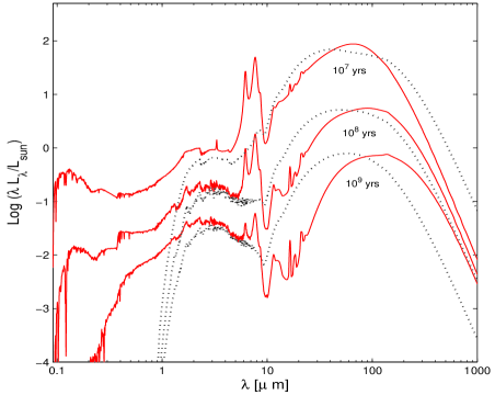
Figure 9: Spectra of dusty SSPs of metallicity $Z=0.02$ calculated with DUSTY (central point source - dotted lines) and with the ray tracing method (distributed source - continuous lines). They are represented at three different ages, from top to bottom: $10$ Myr, $100$ Myr and $1$ Gyr.

In Fig. 9 we compare young dusty SSPs calculated both with DUSTY (central point-source) and the ray tracing technique (distributed source). Both SSPs have the solar metallicity, the same optical depth and matter profile of the cloud, and the same dust properties. The geometry is the origin of the lack of stellar emission for the dusty SSPs calculated with the central point-source model. All the stars are indeed embedded in a medium of high optical depth so that no stellar light can escape from it. Even if in some cases of highly embedded sources this could be a good approximation, in general it is not realistic, because we can easily conceive that in a real environment with ongoing star formation, young stars can be formed everywhere even near the edges of the MCs. Such stars are therefore less obscured by dust. The ray-tracing method with the stars distributed into the cloud can easily handle this situation thus allowing a fraction of the stellar light to be always detectable. This is a net advantage with respect to the central point-source approximation. As a matter of facts, there is observational evidence for contributions to the UV-NIR flux from bursts of young stars as discussed by Takagi et al. (see the discussion by 2003). The central point-source model is not able to simulate properly this contribution, which is instead nicely described by young stars being distributed all across the cloud. Anyway, as the point-source model can reasonably simulate highly obscured and concentrated populations of stars, we plan to introduce also this case in our library of SEDs.

7 The radiative transfer problem

7.1 The ray tracing method

To solve the radiative transfer equation we use the robust and simple technique otherwise known as the ”ray tracing” method (Band & Grindlay, 1985; Takagi et al., 2003). The method solves the radiative transfer equation along a set of rays traced throughout the inhomogeneous spherically symmetric source. Thanks to the spherical symmetry of the problem, it is possible to calculate the specific intensity of the radiation field at a given distance from the center of the MC by suitably averaging the intensities of all the rays passing through that point (Band & Grindlay, 1985). The geometry of the problem is best illustrated in Fig. 10 which shows a section of a spherically symmetric MC. We consider a discrete set of $N$ concentric spheres (circles on the projection) and an equal number of rays indicated by the parameter $j$ running from $j$=1 to $j$=N. The specific intensity is calculated at all intersections of the generic ray $j$ with the generic circle (sphere). The number of intersections $i$ increases from 1 for $j$=$N$ to $2(N-1)+1$ according to the rule $i$=$2(N-j)+1$. The equation of radiative transfer for specific intensity $I_{\lambda}\left(y,x\right)$ along a ray can be written as

$$\frac{dI_{\lambda}\left(y,x\right)}{dx}=-n_{H}\left(r\right)\sigma_{ext}\left(\lambda\right)\left[I_{\lambda}\left(y,x\right)-S_{\lambda}\left(r\right)\right]$$ (29)

where $y$ is the impact parameter, i.e. the distance of the generic ray $j$ from the ray passing through the center, and $x$ is the coordinate along the ray; $n_{H}\left(r\right)$ is the number of hydrogen atoms per cubic centimeter; $\sigma_{ext}\left(\lambda\right)$ is the cross section of extinction for hydrogen atoms defined in eqn. (7); finally, $S_{\lambda}\left(r\right)$ is the source function at a given radius. We include the metallicity dependence for the composition of the MCs (on the notion that a generation of newly born stars shares the same metallicity of the surrounding MCs) as follows: for metallicities $Z\geq 0.015$ we use the extinction curve of the MW for dense regions, characterized by a reddening parameter as high as is $R_{V}=5.5$; for metallicities in the interval $0.005\leq Z\leq 0.015$ we adopt the extinction curve of the LMC; finally, for metallicities lower than $Z\leq 0.005$ we use the typical extinction curve of the SMC.

In order to solve eqn. (29), following Rowan-Robinson (1980) we split the specific intensity in three components: $I_{\lambda}=I_{\lambda}^{\left(1\right)}+I_{\lambda}^{\left(2\right)}+I_{\lambda}^{\left(3\right)}$, where $I_{\lambda}^{\left(1\right)}$ is the light from the stellar source, $I_{\lambda}^{\left(2\right)}$ is the light scattered by the grains, and, $I_{\lambda}^{\left(3\right)}$ is the radiation coming from the thermal emission of the grains. It is possible to calculate the contribution from each component, if the optical properties of the dust grains do not depend on their temperature. This is indeed the case of the optical coefficients taken from Draine & Lee (1984), Laor & Draine (1993) and Li & Draine (2001). As we are in spherical geometry only a radial grid needs to be specified. For each impact parameter $y_{j}=r_{j}$, $I_{\lambda}^{\left(1\right)}$ is calculated and stored at each intersection of the $j$-th ray with the spheres (circles) (as shown in Fig. 10), where the stellar source function $S_{\lambda}^{\left(1\right)}\left(r\right)$ is taken from Takagi et al. (2003).

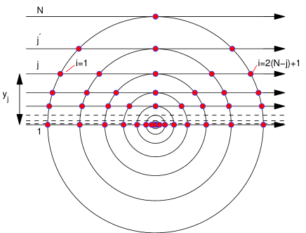
Figure 10: Two dimensional section of a dusty MC. A set of $N$ rays is traced each one tangent to one of N concentric spherical surfaces of a radial grid with $N=10$ and thicker spacing toward the center of the cloud. The specific intensity is calculated for each ray at each point when the ray penetrates one of the surfaces. The $j$-th ray cross $N-j$ surfaces in $2\left(N-j\right)+1$ points. $y_{j}$ is the impact parameter of the $j$-th ray.

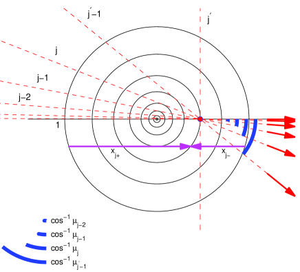
Figure 11: Two dimensional section of a dusty MC. A set of $N$ spherical surfaces of a radial grid with $N=10$ is shown. The average intensity is calculated for the point $j^{\prime}$ by using all the rays from $1$ to $j^{\prime}-1$, each rays weighted for the cosine of the angle with the radial vector. For each ray we have two contributes, one for each direction, $x_{j_{-}}$ and $x_{j_{+}}$.

Once the matrix $I_{\lambda}^{\left(1\right)}\left(y_{j},x_{i+1}\right)$ is calculated, it is possible to obtain the mean intensity $J_{\lambda}^{\left(1\right)}\left(r_{j}\right)$ at a given radius performing an integration over the cosine grid $\mu_{j}$ as displayed in Fig. 11. We have now to calculate the contribution of $I_{\lambda}^{\left(2\right)}$ and $I_{\lambda}^{\left(3\right)}$ to $J_{\lambda}$. The source function of the $n$-times scattered light is

$$S_{\lambda,n}^{\left(2\right)}\left(r,\overrightarrow{n}\right)=\frac{\omega_{\lambda}}{4\pi}\int\phi\left(\overrightarrow{m},\overrightarrow{n}\right)I_{\lambda,n-1}^{\left(2\right)}\left(r,\overrightarrow{m}\right)d\Omega$$ (30)

where $I_{\lambda,n-1}^{\left(2\right)}$ is the associated specific intensity. The function $\phi\left(\overrightarrow{m},\overrightarrow{n}\right)$ is the phase function, which yields the distribution of photons scattered in different directions. For the sake of simplicity we assume isotropic scattering so that $\phi\left(\overrightarrow{m},\overrightarrow{n}\right)=1$. The total intensity of scattered light is obtained by adding all scattering terms $I_{\lambda}^{\left(2\right)}=\sum_{n}I_{\lambda,n}^{\left(2\right)}$. We start from $I_{\lambda}^{\left(1\right)}$, which can be considered as the $0$-times scattered light, to obtain the source function of $1$-times scattered light (Takagi et al., 2003) and the average specific intensity for each spherical concentric shell. We derive $S_{\lambda,n}^{\left(2\right)}\left(r\right)$ and repeat these steps, calculating the scattering terms of higher order. By taking a sufficiently large number of steps, six are sufficient (Takagi et al., 2003), the energy conservation is secured.

Finally, we need the source function for the infrared emission of dust. We take also dust self-absorption into account: for high optical depths such as the ones of MCs, the infrared photons can be absorbed and self-absorption has to be considered. An iterative procedure is required until the energy conservation is reached: using the mean intensities of direct and scattered light, $J_{\lambda}^{\left(1\right)}\left(r\right)$ and $J_{\lambda}^{\left(2\right)}\left(r\right)$, the dust source function for the $1$-th iteration $S_{\lambda,1}^{\left(3\right)}\left(r\right)$ together with the corresponding average intensity $J_{\lambda,1}^{\left(3\right)}\left(r\right)$ are obtained. Starting from $J_{\lambda,1}^{\left(3\right)}\left(r\right)$, we iterate the procedure to get the thermal emission of dust $J_{\lambda,n}^{\left(3\right)}\left(r\right)$ by means of the the local radiation field $J_{\lambda}^{\left(2\right)}\left(r\right)+J_{\lambda}^{\left(1\right)}\left(r\right)+J_{\lambda,n-1}^{\left(3\right)}\left(r\right)$. The dust emission is calculated as described in Sect. 3.1 with the GDP model. Therefore, the source function of dust is given by

$$S_{\lambda,1}^{\left(3\right)}\left(r\right)=\frac{1}{\sigma_{ext}\left(\lambda\right)}\left(j_{\lambda}^{small}+j_{\lambda}^{big}+j_{\lambda}^{PAH}\right)$$ (31)

where $j_{\lambda}^{small}$, $j_{\lambda}^{big}$ and $j_{\lambda}^{PAH}$ are the contributions to the emission by small grains, big grains and PAHs, respectively.

7.2 Optical depth of the cloud

Key parameter of the radiative transfer is the optical depth $\tau_{\lambda}$ defined as

$$\tau_{\lambda}=\int\nolimits_{S}k_{\lambda}\rho ds$$ (32)

where $k_{\lambda}$ is the extinction coefficient, $\rho$ is the density of the matter and $S$ is the thickness of the cylinder of matter along which we integrate. Eqn. (32) can be recast as follows

$$\tau_{\lambda}=\int_{0}^{R_{MC}}n_{H}\left(r\right)\sigma_{\lambda}\left(r\right)dr$$ (33)

where $n_{H}\left(r\right)$ is the number density of $H$ atoms and $\sigma_{\lambda}\left(r\right)$ is the extinction cross section (scattering plus absorption).

In order to calculate the thickness of the shell, we need an estimate of the mass $M_{MC}$ and the radius $R_{MC}$ of the cloud. Silva et al. (1998) adopt a ”typical” MC of given mass and radius. However, there is plenty of evidence that MCs span large ranges of masses and radii in which the low mass and small radius ones are by far more numerous. Therefore, in a realistic picture of the effects of dust clouds, the mass and radius distributions of these latter should be taken into account thus requiring that large ranges of optical depths are considered. We start calculating the optical depth for a cloud with a generic mass $M_{MC}$ and radius $R_{MC}$. From the identity $\rho_{g}\left(r\right)=\rho_{H}\left(r\right)+\rho_{He}\left(r\right)+\rho_{Z}\left(r\right)$ with $\rho_{Z}\left(r\right)$, $\rho_{H}\left(r\right)$, $\rho_{He}\left(r\right)$ densities of metals, hydrogen, and helium, respectively, after putting $\rho_{H}\left(r\right)$ into evidence and neglecting $\rho_{Z}\left(r\right)/\rho_{H}\left(r\right)$ we get:

$$\rho_{H}\left(r\right)\sim\frac{\rho_{g}\left(r\right)}{\left(1+\frac{\displaystyle\rho_{He}\left(r\right)}{\displaystyle\rho_{H}\left(r\right)}\right)}\sim\rho_{0,g}\frac{\left[1+\left(\frac{\displaystyle r}{\displaystyle r_{c,g}}\right)^{2}\right]^{-\gamma_{g}}}{\left(1+\frac{\displaystyle\rho_{He}\left(r\right)}{\displaystyle\rho_{H}\left(r\right)}\right)}$$ (34)

We can now reasonably assume that the hydrogen and helium distributions have the same scale radius, so that $\rho_{He}\left(r\right)/\rho_{H}\left(r\right)=\rho_{He,0}/\rho_{H,0}$ does not depend on the coordinate $r$. Dividing eqn. (34) by the mass of the $H$ atom $m_{H}$ and supposing that $\sigma_{\lambda}\left(r\right)$ does not depend on the coordinate $r$ along the cylinder of matter we derive

$$\tau_{\lambda}=\frac{\sigma_{\lambda}\rho_{0,g}}{\left(1+\frac{\displaystyle\rho_{He,0}}{\displaystyle\rho_{H,0}}\right)m_{H}}\int_{0}^{R_{MC}}\left[1+\left(\frac{r}{r_{c,g}}\right)^{2}\right]^{-\gamma_{g}}dr$$ (35)

Setting $z=r/r_{c,g}$ and introducing the parameter $\eta=r_{c,d}/r_{c,s}=r_{c,g}/r_{c,s}$ – with the ratio of the cloud radius $R_{MC}$ to the scale radius of the gas component given by $R_{MC}/r_{c,g}=10^{2.2}\cdot(r_{c,s}/r_{c,g})=10^{2.2}/\eta$ – and $\gamma_{g}=1.5$ we obtain

$$\tau_{\lambda}=\frac{\sigma_{\lambda}\rho_{0,g}R_{MC}}{\left(1+\frac{\displaystyle\rho_{He,0}}{\displaystyle\rho_{H,0}}\right)m_{H}}\times\frac{\eta}{10^{2.2}}\int_{0}^{\frac{10^{2.2}}{\eta}}\left(1+z^{2}\right)^{-1.5}dz$$ (36)

The normalization constant $\rho_{0,g}$ is derived by integrating the density law for a MC given by eqn. (28) over its volume and using the identity

$$M_{MC}=4\pi\,\rho_{0,g}\,(r_{c,g})^{3}\int_{0}^{R_{MC}/r_{c,g}}{\frac{x^{2}}{(1+x^{2})^{-1.5}}}dx$$ (37)

with $x=r/r_{c,g}$.

The above expression for the optical depth depends only on suitable constants and the dimension-less integral which is a function of $\eta$. Denoting with

$$\Phi\left(\eta\right)=\frac{\eta}{10^{2.2}}\int_{0}^{\frac{10^{2.2}}{\eta}}\left(1+z^{2}\right)^{-1.5}dz$$ (38)

and $K=1/\left[\left(1+\displaystyle\rho_{He,0}/\displaystyle\rho_{H,0}\right)\,m_{H}\right]$, we finally get

$$\tau_{\lambda}=K\sigma_{\lambda}\rho_{0,g}R_{MC}\,\Phi\left(\eta\right)$$ (39)

The parameter $\eta$ describes the dust distribution: for $\eta=1000$ we have a nearly uniform distribution of dust in which stars are embedded, whereas for $\eta=1$ stars and dust in the MCs have the same distribution. Typical values of $\Phi\left(\eta\right)$ are $\Phi\left(\eta\right)=0.0063,0.063,0.534,0.988$ as $\eta$ goes from 1 to 10, 100, 1000, respectively. Following Takagi et al. (2003) who reproduced the central star forming regions of M82 and Arp220 using a nearly uniform distribution of dust ($\eta=1000$), we adopt the same value for this parameter. Looking at the optical depth of the cloud we have just defined, there are other considerations to be made about the geometry of the system. Both the mass $M_{MC}$, via the central density $\rho_{0,g}$, and the radius $R_{MC}$ of the cloud are present in eqn. (39). The first problem to deal with is that masses and radii of real MCs span large ranges of values. This problem will be addressed in detail in Sect. 7.3. Second, in all the relationships we have been using in so far to define the final expression for the optical depth, the total mass of the stars embedded into the MC does not play any role. This is obvious because the optical depth depends only on the dust-fog in which the stars-candles are embedded, and not on the candles themselves. So, which star mass $M_{\star}$ has to be considered for a cloud with mass $M_{MC}$ and radius $R_{MC}$? There is no easy answer to this problem. We start considering that our MCs spectra will be eventually used to build integrated spectra of galaxies. Therefore, we need normalized MCs spectra to be convolved with the SFH of the galaxy. The simplest way we can achieve the goal is to consider as candle a SSP of $M_{\star}=1M_{\odot}$. We keep fixed the optical depth of the cloud calculated with eqn. (39) using the real dimensions of the cloud and then we re-scale the radius of the cloud according to the relation (Takagi et al., 2003)

$$R_{MC}^{\prime}=10R_{s}\left(\frac{M_{\star}}{10^{11}M_{\odot}}\right)^{0.5}$$ (40)

where $R_{MC}^{\prime}$ (in kpc) is the normalized radius corresponding to the adopted mass $M_{\star}$ (for an arbitrary star mass $M_{\star}$, the radius $R_{MC}$ has to be suitably scaled). As noticed by Takagi et al. (2003), when the optical depth and the scaling parameter $R_{s}$ are kept fixed, the relative shape of the SED remains unchanged for different masses $M_{\star}$. The only effect of varying $M_{\star}$ is to produce a higher energy output, but the SED remains the same.

7.3 The mass spectrum of MCs

As already mentioned, there is observational evidence that the MCs span large ranges of masses and radii. Let us assume now that masses and radii of molecular clouds obey the distribution laws $dN/dM_{MC}=A_{M}M_{MC}^{-\alpha}$ and $dN/dR_{MC}=A_{R}R_{MC}^{-\beta}$ where the normalization constants $A_{R}$ and $A_{M}$ can be determined integrating over the distributions once the lower and upper limits are specified. We split the mass and radius intervals in a discrete number of bins, and indicate with $n$ and $m$ the number of the mass and radius bins, respectively. The normalized number $N_{i}\left(M_{MC}\right)/N$ of clouds into the $i$ mass bin of $n$ bins and the number of clouds $N_{i}\left(R_{MC}\right)/N$ into the $i$ radius bin of $m$ bins can be easily obtained. They are independent of the normalization constant $A_{R}$ and $A_{M}$. The sum over all the bins is of course normalized to unity. The fraction of molecular clouds with mass belonging to the $i$-th bin of $n$ bins and radius belonging to the $j$-th bin of $m$ bins will be

$$f\left(M_{i},R_{j}\right)=\frac{N_{i}\left(M_{MC}\right)}{N}\times\frac{N_{j}\left(R_{MC}\right)}{N}$$ (41)

According to eqn. (39), for $\eta=1000$ the function $\Phi\left(\eta\right)\thickapprox 1$ and the central density $\rho_{0,g}$ is nearly equal to the mean density because dust is almost uniformly distributed, i.e. $\rho_{0,g}\thickapprox\overline{\rho}_{g}$. Recalling that $\overline{\rho}_{g}=3M_{MC}/\left(4\pi R_{MC}^{3}\right)$, we obtain $\tau_{\lambda}\varpropto M_{MC}/R_{MC}^{2}$. This means that for each ratio $M_{MC}/R_{MC}^{2}$ a different value of the optical depth is expected. Furthermore, splitting the range of optical depths in $k$ bins, it may happen that different combinations of $M_{MC}$ and $R_{MC}$ yield a similar value of $\tau_{\lambda}$. As a consequence of this, different pairs of bins $\left(i,j\right)$ may give their fractional contribution to the same bin $\tau\left(i,j\right)$ of the optical depth.

The limits of the mass and radius distributions can be inferred from the observational surveys of Solomon et al. (1987) of galactic MCs and the analysis made by Elmegreen & Falgarone (1996). Typical values are: $R_{up}\simeq 70$ pc, $R_{low}\simeq 5$pc, $M_{up}\simeq 3\times 10^{6}M_{\odot}$ and finally $M_{low}\simeq 4\times 10^{4}M_{\odot}$. The exponents of the mass and radius distribution, $\alpha$ and $\beta$ respectively, are taken from Elmegreen & Falgarone (1996). We have $\beta\simeq 3.3\pm 0.3$ for the radii distribution and $\alpha\simeq-1.8$ for the mass distribution. These power-laws imply that not all the optical depths $\tau\left(i,j\right)$ will have the same weight, but those falling in suitable $k$-bins will weigh more so that the whole range can be reduced to these values. This is clearly shown in Fig. 12 where the discrete function $f\left(M_{i},R_{j}\right)$ is plotted over $15$ radius bins and $15$ mass bins and the $f(1,1)$ bin weights much more than the other ones. However, there is a strong dependence on the lower limits of the distribution laws we have adopted, i.e. the one holding for the MW, and it is likely that in different environments, such as strong star forming galaxies, the distribution laws may be different. Therefore, a realistic model of galaxies should include MCs with an ample range of optical depths and also different laws for the mass and size of the MCs. For the purposes of this study, we limit ourselves to the distribution laws holding for the MW. With these distribution laws and using 15 bins, the $f(1,1)$ bin weighs about $50\%$ of the total, as shown in Fig. 12. Thanks to this, for the time being we can simplify the problem and take only one optical depth as a free parameter representative of the whole range, both in star forming regions (Sect. 9) and galaxies (Piovan et al., 2005).

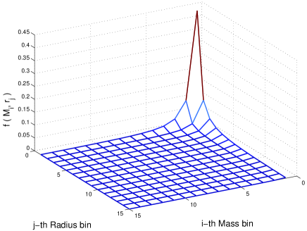
Figure 12: Three dimensional plot of the function $f\left(M_{i},R_{j}\right)$ for $15$ mass bins and $15$ radius bins. The first bin corresponds to the lowest mass and radius of the distributions.

8 SEDs of young SSPs surrounded by MCs

In this section, we present the SEDs of young SSPs in which the effects of dust around are included according to the prescriptions of Sect. 7 and compare them with the standard case in which dust is neglected. For each metallicity the analysis is limited to the most probable bin $f(1,1)$ of the mass and radius distribution of MCs. The optical depth of this bin is about $\tau_{V}=35$ for the solar metallicity, $\tau_{V}=10$ and $\tau_{V}=5$ for the LMC and SMC metallicities (extinction curves). The scaling parameter for the MC dimensions is $R=1$, while the total carbon abundance per H nucleus in the log-normal populations of very small carbonaceous grains, $b_{c}$, has been fixed to a value slightly above the mean value of the allowed range. Finally, the treatment of ionization is as in Weingartner & Draine (2001b). More details will be given in Sect. 8.1 describing the library of young SSPs with dust we have calculated.

We begin showing in Fig. 13 a SSP with $Z=0.02$ (solar metallicity) and age of $30$ Myr, both in presence and absence of dust. The main effects of dust are soon clear: the cloud in which the young population is embedded absorbs the stellar radiation and returns it in the IR. We may also note here the different contributions by the various components of the specific intensity: direct light, scattered light and dust emission. Passing to discuss the effect of the metallicity, for the sake of brevity we will show results only for $Z=0.02$ (Fig. 14), $Z=0.008$ (Fig. 15), and $Z=0.004$ (Fig. 16).

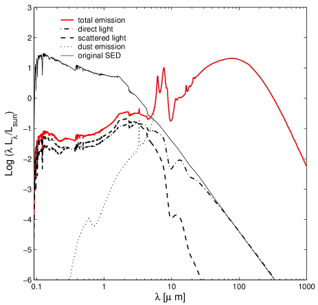
Figure 13: SED of a SSP of $30$ Myr and solar metallicity with and without dust. In the plot we show the original spectrum of the SSP (thin solid line), the total dusty spectrum (thick solid line), the contribution of direct light (dot-dashed line), the contribution of scattered light (dashed line) and, finally, the emission of dust (dotted line).

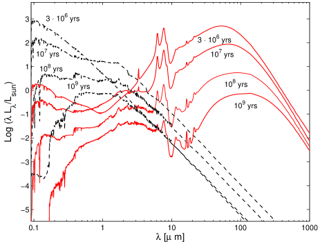
Figure 14: SEDs of SSPs of metallicity $Z=0.02$ without dust (dotted lines) and with dust (solid lines). The spectra are obtained solving the radiative transfer problem by means of the ray tracing method. The SSPs are shown at four different ages, from top to bottom: $3$ Myr, $10$ Myr, $100$ Myr and, finally, $1$ Gyr.

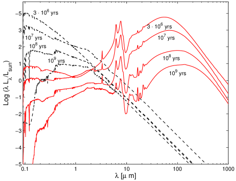
Figure 15: The same as Fig. 14 but for the metallicity $Z=0.008$.

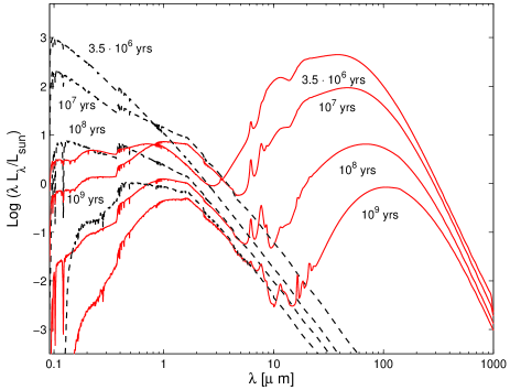
Figure 16: The same as Fig. 15 but for the metallicity $Z=0.004$ and the youngest age that is $3.5$ Myr.

As expected, the SED shift toward the IR is stronger for solar or LMC metallicities, because of the higher optical depth of the MCs (all the other geometrical parameters of the cloud being kept constant). For a given metallicity the peak in IR emission of cold dust shifts toward shorter wavelengths at decreasing age of the SSP, because the intensity of the radiation field gets higher. For each shell of the radial grid in which a MC has been split, we calculate the ionization state of PAHs. The Weingartner & Draine (2001b) model yields SEDs of very young SSPs in which the PAHs are almost fully ionized and the profile of aromatic infrared bands of PAHs (AIBs) is very close to that for the ionized cross sections, as shown by Figs. 14, 15 and 16. At increasing age and hence decreasing radiation field, the profile of AIBs shifts to that of neutral cross section because more and more PAHs become neutral. For the lowest metallicities the contribution of PAHs becomes small because of the small percentage of carbonaceous grains in the adopted extinction curve (the one for SMC). Furthermore, at decreasing age, AIBs become weaker due to the combined effects of the lower optical depth and higher radiation field which cause emission by hot dust in the same wavelength interval of AIBs.

8.1 A library of young SSPs surrounded by MCs

Dealing with theoretical spectra of young SSPs embedded into dusty MCs is a cumbersome affair as a large number of parameters is involved. First, we have those related to dust and its composition (still uncertain), together with those of the optical properties and distribution laws of the grains. Second, we have the geometrical parameters introduced to solve the radiative transfer in a medium with sources distributed in it. Although one could simply take a sort of prototype MC to be inserted in population synthesis studies, it is more physically grounded and close to reality to create and explore in some detail the space of parameters.

First of all, let us discuss the optical depth $\tau_{\lambda}$ and the scaling factor $R$ of MCs (the latter fixing their size). For more details about $R$ and $\tau_{\lambda}$ see also Takagi et al. (2003).

$\tau_{\lambda}$: the optical depth, see eqn. (39), is the main parameter of the radiative transfer problem. Its effect on the spectrum emitted by the MC is simple to describe: if the optical depth is high, more energy is shifted toward longer wavelengths. This amount of energy first quickly increases at increasing optical depth, then becomes less sensitive to $\tau_{\lambda}$ and even tends to flatten out for high $\tau_{\lambda}$. This can be seen in Figs. 14 and 15, where even if the optical depth is different, yet it is high enough to show the above effect. The optical depth depends on the mass and radius of the MC (the geometrical parameters) and different distribution laws for masses and radii lead to different optical depths. The ideal case would be to set up a library of SSPs covering an ample range of optical depths. Because of the high computational time required, the present release of the library is limited to two values of the optical depth for each metallicity, namely $\tau_{V}=35$ and $\tau_{V}=5$.

$R$: the scaling parameter $R$ has been introduced because the mass $M_{\star}$ contained inside a MC has been normalized to $1\,M_{\odot}$, in view of the use of these SSPs in evolutionary population synthesis models for galaxies. $R$ links the mass of the sources of radiation to the dimension of the cloud, as described in Sect. 7.2. There is no effect of varying $R$ over the part of the SED given from the absorbed stellar emission. The only effect of $R$ is to change the position of the FIR peak due to dust emission. A ideal MC scaled with a larger value of $R$ will have a lower temperature profile of the grains because of the bigger dimensions. Accordingly, the FIR peak of dust emission will simply shift to longer wavelengths. This effect is entangled with the age effect, because for older populations the radiation field will be weaker and the FIR peak will undergo a similar shift to longer wavelengths.

Let us now examine the parameters controlling the MIR region of the spectrum, i.e. the intensity of PAH emission and the AIB profiles.

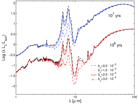
Figure 17: PAH emission as a function of the parameter $b_{C}$. The MIR-FIR region is shown for two young dusty SSPs of $10^{7}$ and $10^{8}$ Myr and metallicity $Z=0.02$. Four values of $b_{C}$ are taken into account, going from $0\cdot 10^{-5}$ until $3\cdot 10^{-5}$, the upper limit for the $R_{V}=5.5$ extinction curve (Weingartner & Draine, 2001a). The other parameters are kept fixed, $R=1$, $\tau=35$ and the ionization model of Weingartner & Draine (2001b).

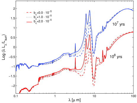
Figure 18: PAH emission in function of the parameter $b_{C}$. The MIR-FIR region is shown for two young dusty SSPs of $10^{7}$ and $10^{8}$ Myr and metallicity $Z=0.008$. Three values of $b_{C}$ are taken into account, going from $0\cdot 10^{-5}$ until $2\cdot 10^{-5}$, the upper limit for the average LMC extinction curve, as proposed in Weingartner & Draine (2001a). The other parameters are kept fixed, $R=1$, $\tau=35$ and ionization model of Weingartner & Draine (2001b).

$b_{C}$: this parameter is the total C abundance (per H nucleus) in the two log-normal distribution laws of very small carbonaceous grains. Even if other distribution laws for the grain dimensions can be used, our preference goes to the Weingartner & Draine (2001a) law because it has been proved to provide excellent fits to the extinction curves and it contains the contribution of very small grains to carbon abundance as a free parameter. Only an upper limit to the parameter $b_{C}$ can be derived and all the values lower than or about equal to this upper limit are possible (see Sect. 2). However the exact value of $b_{C}$ bears very much the PAH emission in the MIR. At increasing $b_{C}$, the AIBs are more pronounced with higher flux levels, while the flux in the UV-optical region and the shape of the absorbed stellar emission remain unchanged as the extinction curve is exactly the same for different values of $b_{C}$. At decreasing $b_{C}$, the emission in the FIR slightly increases (the total energy budget has clearly to be conserved) because the global abundance of $C$ is fixed, and the distribution of the grains has to compensate for the small number of VSGs with respect to the higher number of BGs. In Figs. 17 and 18 we show the effect of varying $b_{C}$ on the emission of two young dusty SSPs of $10^{7}$ and $10^{8}$ Myr both for the metallicities $Z=0.02$ and $Z=0.008$. At increasing $b_{C}$, the AIB emission increases, whereas the FIR emission goes in the opposite way. In our library, four values of $b_{C}$ for solar or super-solar metallicities are considered, three values are taken into account for the LMC metallicity, and only one value is explored for the SMC and lower metallicities (see also Weingartner & Draine, 2001a).

PAH ionization: together with $b_{C}$, there is another parameter affecting the emission of PAHs to be taken into account, in order to match also the complicate profiles of the AIBs, i.e. the ionization state of the PAHs. The profile of the bands depends indeed on the PAH ionization, because the optical properties are different for ionized and neutral PAHs as been discussed in Sect. 3. The ionization is calculated for each spherical shell of a MC. It strongly depends on the age of the SSP: passing from profiles of ionized PAHs for the youngest populations (because of the strong radiation field) to those of neutral PAHs at old ages (because of the weaker radiation field).

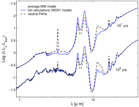
Figure 19: PAH emission as a function of the ionization model. The MIR-FIR region is shown for two young dusty SSPs of $10^{7}$ and $10^{8}$ Myr and metallicity $Z=0.02$. Three models of ionization are taken into account as indicated.

In order to fully explore the space of parameters, three ionization models are considered. The first one is by Weingartner & Draine (2001b). The second model strictly follows the same ionization profile calculated in Li & Draine (2001) for the diffuse ISM of the MW. The third model simply takes into account only the optical properties of neutral PAHs. In this way we can study a sequence of ionization states going from strongly ionized to almost neutral. For the second and the third model there is no change of the profile of the AIBs at varying the age of the underlying SSP as instead it happens in the first model. In Fig. 19 we compare the results for the three ionization models showing the emission of two young dusty SSPs with different age, i.e. $10^{7}$ and $10^{8}$ Myr, and the same metallicity $Z=0.02$ (all other parameters are kept fixed). The PAH ionization has no effect on the UV-optical and FIR emission because the distribution of the grains is the same and their optical properties in these wavelength intervals do not depend on the ionization state. In the MIR we can notice that, as expected, the models with more ionization have more enhanced AIBs at $6,2$ and $7.7\,\mu m$ and $8.6\mu m$, and weaker AIBs at $3.3\,\mu m$ and $11.5\,\mu m$. Clearly, the neutral model, has the strongest AIB at the $3.3\,\mu m$.

8.2 Evaporation of the MCs

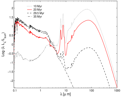
Figure 20: SEDs of a SSP of metallicity $Z=0.02$ from the age of $10$ Myr (dashed line) to the age of $35$ Myr (dot-dashed line). Two intermediate ages are shown of $20$ Myr (continuous line) and $29.5$ Myr (dashed line), respectively. The parameter $t_{0}$ is set equal to 15 Myr.

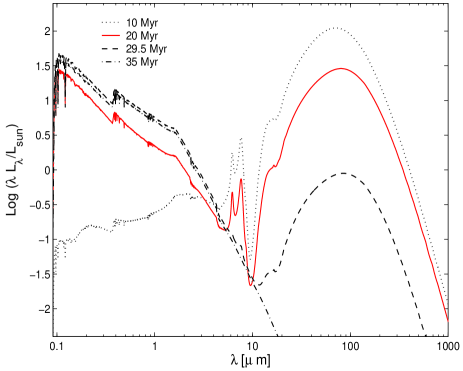
Figure 21: The same as Fig. 20 but for the metallicity $Z=0.004$.

Before using the SED of young dusty SSPs to derive the SED of galaxies, an important aspect has to be clarified. How long does it take to evaporate the MC surrounding a new generation of stars? The subject must be clarified in advance, because what we have been doing so far is only to take the energy emitted by a SSP and inject it into a MC to be re-processed by dust: we have not specified the evolution of the MCs, which are most likely to dissolve by the energy input of the stars underneath. Following Silva et al. (1998), the process can be approximated by gradually lowering as function of time the amount of SSP flux that is reprocessed by dust and increasing the amount of energy that freely escapes from the MC. This is, of course, a rough approximation of the real situation in which the energy input from supernovae and massive stars gradually sweep away the parental gas and dust. A more realistic approach should take into account the energy input coming from supernovae explosions and massive stars and compare it to the binding energy of the gas.

Let us denote with $f_{DSSP}$ the fraction of the SSP luminosity that is reprocessed by dust and with $t_{0}$ the time scale for a MC to evaporate

$$f_{DSSP}=\left\{\begin{array}[]{llll}1&&&\quad t\leq t_{0}\\ 2-t/t_{0}&&&\quad t_{0}<t\leq 2t_{0}\\ 0&&&\quad t\geq t_{0}\end{array}\right.$$ (42)

Accordingly, the fraction of SSP luminosity that escapes without interacting with dust is $f_{SSP}=1-f_{DSSP}$.

The parameter $t_{0}$ will likely depend on the properties of the ISM and type of galaxy in turn. Plausibly, $t_{0}$ will be of the order of the lifetime of massive stars, say from 100 to 10 $M_{\odot}$, that first explode as supernovae and whose ages range from $3$ to $100$ Myr. However, the real timescale is likely to be much close to the shortest value, i.e. the lifetime of the most massive supernovae in the SSP, for a low density environment like spiral galaxies with a low star formation rate, while it will be much close to the longest value for a high density environment like the star forming central regions of starburst galaxies. For the sake of illustration, in Figs. 20 and 21 we show the gradual transition of SSPs with different metallicity, $Z=0.02$ and $Z=0.04$, respectively, from fully embedded in their original MCs to free of dust. In all the cases, the optical depth is $\tau_{V}=35$ and $R=1$, $b_{c}$ is fixed at the high value holding for MW and at the only available value for the SMC and, finally, the Weingartner & Draine (2001b) ionization model is fully used. The SEDs are displayed at four different ages, $10$, $20$, $29.5$, and $35$ Myr. The parameter $t_{0}$ is fixed to $t_{0}=15$ Myr.

At the age of 10 Myr, the SSPs are fully enshrouded by dust and no evolution of the fluxes is still simulated (dotted lines in Figs. 20, and 21). At the age of 35 Myr, the SSPs are no longer surrounded by MCs, their SED is the one of a bare classical SSP without dust contribution of extinction and emission (dot-dashed lines in Figs. 20, and 21). For the other two values of the age the SED is intermediate to the previous ones. The trend is as follows: at the beginning the stars are heavily masked but when the age of the SSP enter the range between $t_{0}\leq t\leq 2t_{0}$ part of the energy is transferred to the optical range and part remains in the IR. As the stars become older, the quantity of energy emitted in the IR diminishes and eventually disappears when $t\geq 2t_{0}$.

9 Comparison with observational data

To test our model for dusty SSP we compare the theoretical SEDs with the observational data for the central star forming regions of some local starburst galaxies. A simple picture aimed at explaining most of the observational constraints for starbursters has been proposed by Calzetti (2001). The newly born stars, likely still embedded in their parental MCs, are concentrated in the centre of the galaxy, surrounded by long-lived less massive stars wrapped by a diffuse dusty medium. Clearly, the real distribution of stars and dust will be much more complicated, with clumps and asymmetries. If the burst of star formation is strong enough, the flux coming from the central region of the galaxy (small-aperture data) is dominated by the obscured light coming from the new generations of stars. In this way, if we limit ourselves to study small central regions of starbursters, to a first approximation we can try to reproduce the observed SED with an obscured SSP of suitable mass. It is clear, however, that if the burst lasts longer than the life of the most massive stars (Calzetti, 2001), the stellar populations in the central region under examination are no longer coeval. Rather they are a mix of spatially concentrated very young stars superimposed to older and more dispersed foreground stars. The longer or the weaker the burst of star formation, the higher is the influence of the older generations of stars on the resulting SED and the weaker the physical significance of the SSP approximation. Nevertheless, despite of these remarks, the comparison of our SSP SEDs with the SED from the central dusty star forming regions of local starbursters is the best tool to our disposal to validate the model.

9.1 Central region of Arp 220

Arp $220$ is a very bright object in the Local Universe, classified by Arp (1966) as a peculiar galaxy. The interest in this galaxy became very strong when the IRAS satellite revealed that it is a powerful source of FIR emission. Today, we know that Arp $220$ is the nearest and most thoroughly studied example of UltraLuminous InfraRed Galaxies (ULIRG), objects with an infrared luminosity $L_{IR}\geq 10^{12}L_{\odot}$ (Sanders et al., 1988). The redshift of the galaxy, taken from the NED database is $z=0.01813$, which for the Hubble constant $H_{0}=72$ km/s/Mpc yields a distance of about $76$ Mpc. This value is fully consistent with the distances proposed in Soifer et al. (1987) and in Spoon et al. (2004). Wynn-Williams & Becklin (1993) showed that almost all the MIR flux of Arp$220$ comes from a small central region of about $5^{"}$ aperture. This concentration of the MIR emission has been confirmed by Soifer et al. (1999) comparing the fluxes measured varying the beam size at a fixed MIR wavelength. We take the $5^{"}$ central region of the galaxy, which corresponds to a diameter of about $2$ kpc (Takagi et al., 2003), to test our SSPs.

In Fig. 22 we show the results of our fit obtained using dusty SSPs, with high optical depth $\tau_{V}=35$, compact structure with $R=0.5$ and the SMC extinction curve. The low metallicity extinction curve we have selected agrees with the results by Takagi et al. (2003). Only with a mixture of grains, like the one of the SMC extinction curve, we were able to reproduce the deep absorption features of silicates, the low emission of PAHs and the optical/NIR continuum. So, the fit seems to require relative proportions of grains favouring the grains of silicates with respect to the graphitic ones, like in a flat SMC extinction curve, even if the average metallicity of the environment could be easily supersolar. To clarify the issue we should apply the EPS to chemical models in which the dust abundances (Dwek, 1998, 2005) are followed in detail. As this step is not yet accomplished, work is in progress. The best fit is found for the age of $30$ Myr, a mass of $0.4\cdot 10^{11}M_{\odot}$ and both solar and supersolar metallicity, thus suggesting the present of a high metallicity environment as shown in the right panel of Fig. 22.

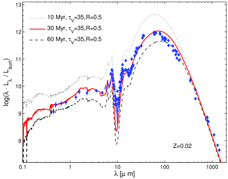
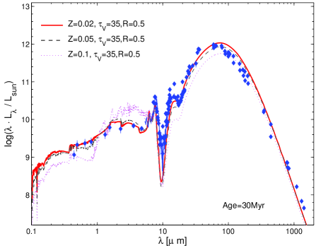
Figure 22: Left Panel: Best fit of the emission from the central region of Arp$220$. We show three SSPs with the ages of $10$, $30$ and $60$ Myr (dotted, continuous and dashed lines respectively). The best fit is for $30$ Myr. Data are taken from Sanders et al. (1988, B, g, r, i), Carico et al. (1990, J, H, K, L). The MIR fluxes are from Spinoglio et al. (1995, MIR), Smith et al. (1989, MIR), Klaas et al. (1997, from MIR to FIR), Wynn-Williams & Becklin (1993, MIR), Tran et al. (2001, 5 - 16 $\mu$m ISOCAM-CVF spectrum). FIR and radio data are from Rigopoulou et al. (1996, sub-mm), Eales et al. (1989, UKIRT sub-mm), Dunne et al. (2000, SCUBA sub-mm), Dunne & Eales (2001, SCUBA sub-mm). Other data are taken from Spoon et al. (2004). Right Panel: The same as in the left panel but for fixed age and varying metallicity. We show three metallicities: $Z=0.02$, $Z=0.05$ and $Z=0.1$ (continuous, dashed and dotted lines, respectively).

9.2 Central region of NGC 253

NGC 253 is a bright starburst galaxy belonging to the Sculptor group, in the direction of the South Galactic Pole. It is perhaps one of the nearest Galaxies besides those of the Local Group. The redshift is $z=0.000804$ (NED), corresponding to the distance $d=3.35$Mpc for $H_{0}=72$ km/s/Mpc.

The central region we have selected is within $15"$ aperture and its SED is centered around the peak of MIR emission. For this region there are available data on the PAH emission from Sturm et al. (2000, ISO-SWS) and Förster Schreiber et al. (2003, ISOCAM) that agree each other, thus confirming the accuracy of the calibrations and setting a strong constraint on the global fit. There are some problems with OAO data (Code & Welch, 1982) covering the UV range, because of the large aperture $10^{{}^{\prime}}$. We scaled the OAO data to the aperture size in usage here. It is clear that a precise correction would require the knowledge of the true UV profile of the galaxy, which is unknown. For this reason, even if the corrected UV level of flux is reproduced, we will give less weight to the UV region looking for the global fit.

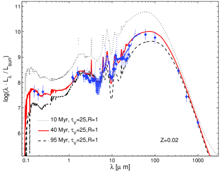
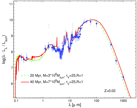
Figure 23: Left Panel: Best fit of the emission from the central region of NGC$253$. We show three SSPs with ages of $10$, $40$ and $95$ Myr (dotted, continuous and dashed lines, respectively). The best fit is for $40$ Myr. Data for the central region are taken and adapted from Code & Welch (1982, UV), Spinoglio et al. (1995, J, H, K, L), Jarrett et al. (2000, J, H, K - 2MASS), Moshir & et al. (1990, IRAS), Chini et al. (1984, sub-mm), Sturm et al. (2000, private communication), Förster Schreiber et al. (2003, private communication). Right Panel: The same as in the left panel but at varying both the age and the mass of the galaxy for the same metallicity.

In the right panel of Fig. 23, we show our best fit obtained with a SSP of solar metallicity, $\tau_{V}=25$, $R=1$, MW extinction curve for dense regions $(R_{V}=5.5)$ and average-low value of the abundance of carbon in the very small carbonaceous grains $(b_{C}=1.0\cdot 10^{-5})$. The ionization model which best agrees with the observations is the one with a dominant neutral component of PAHs. The mass of the population of stars is about $7\cdot 10^{8}M_{\odot}$. In the left panel we show an effect of a sort of age-mass degeneracy: if we can obtain a good fit for a given age and mass, an equally good fit is possible lowering both the age and the mass, because a younger population is more luminous. In spite of this uncertainty, there should be a young population of stars with age of about $30$ Myr and total mass of about $5\cdot 10^{8}M_{\odot}$.

9.3 Central region of M82

The starburst galaxy M$82$ with its companion M$81$ was discovered in 1774 by Johann Bode and independently by Méchain in 1779. He reported them to Messier, who added these two objects to his catalog. The central region of the galaxy, which likely suffered a strong interaction about $10^{8}$ years ago (Förster Schreiber et al., 2003) with its companion M$81$, shows a remarkable burst of star formation activity. The classical distance to M$82$ is $3.25\pm 0.20$ Mpc (Tammann & Sandage, 1968) that makes of M$82$ the nearest and most studied starburst galaxy (see Shopbell & Bland-Hawthorn, 1998, and references therein).

For M$82$ there are many available data for the PAH emission in the MIR region, to which we pay particular attention. They are very useful to constrain the fit to the observed SED of the central region. ISO-SWS data by Sturm et al. (2000, private communication) cover a wide spectral region going from $2.4$ to $45\mu m$. Different SWS full grating scans that are observed with different aperture sizes, going from $14^{"}\times 20^{"}$ to $20^{"}\times 33^{"}$ are patched together. Recently, Förster Schreiber et al. (2003, private communication) observed M$82$ in the MIR range between $5.0$ and $16\mu m$ with ISOCAM on board of ISO. The total field of view was $96^{"}\times 96^{"}$. We have chosen to examine the central M$82$ region of $30^{"}\times 30^{"}$. For this coverage we can use the Förster Schreiber et al. (2003) data (Core plus Disk observations), while Sturm et al. (2000) data with smaller apertures have been properly corrected.

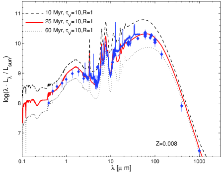
Figure 24: Modelling the SED of the $30^{"}\times 30^{"}$ central region of M$82$. We show three SSPs with ages of $10$, $25$ and $60$ Myr (dashed, continuous and dotted lines, respectively). The best fit is for $25$ Myr. Data for the central region of this galaxy are taken from: NED online database, Johnson (1966, UBVRI), Ichikawa et al. (1995, JHK), Soifer et al. (1987, IRAS), Golombek et al. (1988, IRAS), Rice et al. (1988, IRAS), Klein et al. (1988, FIR and sub-mm), Sturm et al. (2000, private communication), Förster Schreiber et al. (2003, private communication).

In Fig. 24 we show our best fit, obtained with $\tau_{V}=10$, $R=1$, metallicity $Z=0.008$ and the LMC extinction curve. The carbon abundance in small grains is equal to the average $b_{C}=1.0\cdot 10^{-5}$ of current estimates for LMC. The best ionization state of PAHs is the average ionization model for the MW diffuse ISM. All the spectral regions are well reproduced, the major uncertainties being the $18\mu m$ silicates absorption feature and the far UV region where we have no data. The mass obtained from the fit is $M=8\cdot 10^{8}M_{\odot}$.

9.4 Central region of NGC 1808

NGC 1808 is a starburst spiral galaxy in the southern hemisphere sky. The redshift of the galaxy is $z=0.003319$ (NED) which for $H_{0}=72$ km/s/Mpc corresponds to a distance of about $13.82$ Mpc.

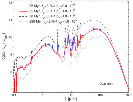
Figure 25: Modelling the SED of the $15^{"}\times 15^{"}$ central region of NGC$1808$. We show three SSPs with ages of $30$, $95$ and $250$ Myr (dashed, thick continuous and dotted lines, respectively). The the best fit is for $95$ Myr for $b_{C}=1.0\cdot 10^{5}$. Another good fit (thin continuous line) with different $b_{C}$ is also shown. Data for this galaxy are taken in the NED online database from Griersmith et al. (1982, JHK), Jarrett et al. (2000, JHK), Glass (1973, HKL), Frogel et al. (1982, MIR, 8-13 $\mu$m), (MIR Förster Schreiber et al., 2003, private communication) and Moshir & et al. (1990, IRAS).

For NGC 1808 we have chosen the region $15^{"}\times 15^{"}$ in the centre of the galaxy. In Fig. 25 we show four models, all calculated for the metallicity $Z=0.008$, optical depth $\tau_{V}=8$, scale radius $R=1$. The best fit is obtained for the age of $95$ Myr and a carbon abundance in the log-normal populations of VSGs of $b_{C}=1.0\cdot 10^{-5}$. A good fit is also possible for a lower abundance $b_{C}=0$ and slightly different age of $85$ Myr (see Fig. 25). In all models, the total stellar mass is $M=5\cdot 10^{9}M_{\odot}$. The case of NGC 1808 is more problematic than the other galaxies we have examined insofar. First, there are no data for the optical region with the desired aperture and the aperture-correction applied to other optical data published in literature is too problematic. Second it is difficult to simultaneously reproduce both the flux level of the PAH emission and the absorption features of silicates at $9.7\mu m$ and $18\mu m$. In our fits the absorption features are too deep. The ideal solution would require an obscuration curve with different abundance of silicates. Finally, some data at sub-mm wavelength would be needed to better constrain the fit. Anyway, the results we have derived suggest a population with an average age of about $100$ Myr. In the case of this galaxy the SSP approximation is perhaps too crude and it should be more appropriate to use of a mix of stellar populations, thus perhaps getting a better fit of both the absorption and emission features in the MIR.

10 Discussion and conclusions

In this study we have presented detailed models of extinction and emission of the diffuse ISM and the application of the most suitable one to the calculation of a library of young dusty SSPs embedded in their parental MCs.

We have analyzed the properties of a dusty ISM having as guide-line of the strategy the cross-checking of the results for extinction and emission and iterating the procedure to contrive the many, somehow unavoidable parameters at work, so that not only unrealistic solutions have been ruled out (they could by generated by the sole fit of the extinction curve) but also additional information on the whole problem has been acquired.

We have adopted two possible models for the distribution of the grains, shortly named MRN and WEI, and explore the consequences. In brief, the MRN-model is a multi-power-law, whose number of components varies with the grain type, whereas the WEI-model is a complicated analytical law suitably corrected for the smaller carbonaceous grains by the sum of two log-normal terms. Again, we followed two methods to derive the temperature distribution of VSGs. The first method is a combination and modification of what has been proposed from Guhathakurta & Draine (1989) for silicate and graphite grains and from Puget et al. (1985) for PAHs, in which we introduced the calculation of the ionization state of PAHs following Weingartner & Draine (2001b). It has been shortly indicated as the GDP-model. The second method, due to Draine & Li (2001) and Li & Draine (2001), is the state-of-the-art of these problems as it stands on the exact statistical solution of the problem. We have referred to it as the LID model. Using the LID and/or GDP emission model coupled with MRN and/or WEI model for the size distribution we have calculated the extinction and emission properties of the average diffuse ISM of the MW, LMC and SMC and compared it with observational data.

Looking at the results from GDP+MRN and GDP+WEI and their comparison with the LID+WEI, we adopt the GDP+WEI model as the most suitable description of the properties of the dusty ISM to be used in dusty SSPs and in the model of galaxy SEDs in presence of interstellar dust (Piovan et al., 2005).

We have applied the model of dusty ISM to calculate the SEDs of young SSPs, in which the effects of dust are taken into account. These are particularly relevant in massive, young stars when still embedded in their parental MCs. We propose a description in which stars, gas and dust in a MC obey three different density profiles each of these characterized by its own scale length. In this context, we derive the optical depth of the MC and apply the ray tracing method to solve the problem of radiative transfer across the MC. We have also explored the parameter space of the MC models. Four parameters have been taken into account, namely the scale radius of the MC and its optical depth (the geometrical parameters), the abundance of carbon in the log-normal populations of very small carbonaceous grains and the ionization state of PAHs, both strongly influencing the PAH emission. Basing on this, we have generated an extended library of young dusty SSPs of different chemical composition and age specifically taylored for galactic population synthesis, the final goal of our study. We tested our SEDs trying to reproduce the observational data of star forming regions in the centre of local starburst galaxies, reaching a good agreement between theory and observation. Libraries of SSPs at varying these parameters are made available to public for future use.

References

- Allain et al. (1996a) Allain T., Leach S., Sedlmayr E., 1996a, A&A, 305, 602
- Allain et al. (1996b) Allain T., Leach S., Sedlmayr E., 1996b, A&A, 305, 616
- Allard & Hauschildt (1995) Allard F., Hauschildt P. H., 1995, ApJ, 445, 433
- Arp (1966) Arp H., 1966, ApJS, 14, 1
- Bakes & Tielens (1994) Bakes E. L. O., Tielens A. G. G. M., 1994, ApJ, 427, 822
- Band & Grindlay (1985) Band D. L., Grindlay J. E., 1985, ApJ, 298, 128
- Bertelli et al. (1994) Bertelli G., Bressan A., Chiosi C., Fagotto F., Nasi E., 1994, A&AS, 106, 275
- Bessell et al. (1991) Bessell M. S., Brett J. M., Scholz M. W. P. R., 1991, A&AS, 89, 335
- Bessell et al. (1989) Bessell M. S., Brett J. M., Wood P. R., Scholz M., 1989, A&AS, 77, 1
- Bressan et al. (1994) Bressan A., Chiosi C., Fagotto F., 1994, ApJS, 94, 63
- Bruzual & Charlot (1993) Bruzual G., Charlot S., 1993, ApJ, 405, 538
- Calzetti (2001) Calzetti D., 2001, PASP, 113, 1449
- Calzetti et al. (1994) Calzetti D., Kinney A. L., Storchi-Bergmann T., 1994, ApJ, 429, 582
- Carico et al. (1990) Carico D. P., Sanders D. B., Soifer B. T., Matthews K., Neugebauer G., 1990, AJ, 100, 70
- Chini et al. (1984) Chini R., Kreysa E., Mezger P. G., Gemuend H.-P., 1984, A&A, 137, 117
- Chiosi et al. (1998) Chiosi C., Bressan A., Portinari L., Tantalo R., 1998, A&A, 339, 355
- Code & Welch (1982) Code A. D., Welch G. A., 1982, ApJ, 256, 1
- Combes et al. (1995) Combes F., Boisse P., Mazure A., Blanchard A., Seymour M., 1995, Galaxies and Cosmology. Galaxies and Cosmology, XVI, 407 pp. 192 figs.. Springer-Verlag Berlin Heidelberg New York. Also Astronomy and Astrophysics Library
- Dale et al. (2001) Dale D. A., Helou G., Contursi A., Silbermann N. A., Kolhatkar S., 2001, ApJ, 549, 215
- Dartois & D’Hendecourt (1997) Dartois E., D’Hendecourt L., 1997, A&A, 323, 534
- Desert et al. (1986) Desert F. X., Boulanger F., Leger A., Puget J. L., Sellgren K., 1986, A&A, 159, 328
- Desert et al. (1986) Desert F. X., Boulanger F., Shore S. N., 1986, A&A, 160, 295
- Devriendt et al. (1999) Devriendt J. E. G., Guiderdoni B., Sadat R., 1999, A&A, 350, 381
- Draine (2003a) Draine B. T., 2003a, astro-ph/0304488
- Draine (2003b) Draine B. T., 2003b, astro-ph/0312592
- Draine (2003c) Draine B. T., 2003c, ARA&A, 41, 241
- Draine (2004) Draine B. T., 2004, in Astrophysics of Dust, Proceedings of the conference held 26-30 May, 2003 at Estes Park, Colorado, USA. Edited by Adolf N. Witt, Geoffrey C. Clayton and Bruce T. Draine. ASP Conference Proceedings, Vol. 309. San Francisco: Astronomical Society of the Pacific, 2004. “Unified Dust Model”
- Draine & Anderson (1985) Draine B. T., Anderson N., 1985, ApJ, 292, 494
- Draine & Lee (1984) Draine B. T., Lee H. M., 1984, ApJ, 285, 89
- Draine & Li (2001) Draine B. T., Li A., 2001, ApJ, 551, 807
- Draine & Sutin (1987) Draine B. T., Sutin B., 1987, ApJ, 320, 803
- Dunne et al. (2000) Dunne L., Eales S., Edmunds M., Ivison R., Alexander P., Clements D. L., 2000, MNRAS, 315, 115
- Dunne & Eales (2001) Dunne L., Eales S. A., 2001, MNRAS, 327, 697
- Dwek (1986) Dwek E., 1986, ApJ, 302, 363
- Dwek (1998) Dwek E., 1998, ApJ, 501, 643
- Dwek (2005) Dwek E., 2005, AIP Conf. Ser, in press
- Eales et al. (1989) Eales S. A., Wynn-Williams C. G., Duncan W. D., 1989, ApJ, 339, 859
- Elmegreen & Falgarone (1996) Elmegreen B. G., Falgarone E., 1996, ApJ, 471, 816
- Förster Schreiber et al. (2003) Förster Schreiber N. M., Genzel R., Lutz D., Sternberg A., 2003, ApJ, 599, 193
- Fioc & Rocca-Volmerange (1997) Fioc M., Rocca-Volmerange B., 1997, A&A, 326, 950
- Fluks et al. (1994) Fluks M. A., Plez B., The P. S., de Winter D., Westerlund B. E., Steenman H. C., 1994, A&AS, 105, 311
- Frogel et al. (1982) Frogel J. F., Elias J. H., Phillips M. M., 1982, ApJ, 260, 70
- Glass (1973) Glass I. S., 1973, MNRAS, 164, 155
- Golombek et al. (1988) Golombek D., Miley G. K., Neugebauer G., 1988, AJ, 95, 26
- Gordon & Clayton (1998) Gordon K. D., Clayton G. C., 1998, ApJ, 500, 816
- Griersmith et al. (1982) Griersmith D., Hyland A. R., Jones T. J., 1982, AJ, 87, 1106
- Guhathakurta & Draine (1989) Guhathakurta P., Draine B. T., 1989, ApJ, 345, 230
- Ichikawa et al. (1995) Ichikawa T., Yanagisawa K., Itoh N., Tarusawa K., van Driel W., Ueno M., 1995, AJ, 109, 2038
- Ivezic & Elitzur (1997) Ivezic Z., Elitzur M., 1997, MNRAS, 287, 799
- Jarrett et al. (2000) Jarrett T. H., Chester T., Cutri R., Schneider S., Skrutskie M., Huchra J. P., 2000, AJ, 119, 2498
- Johnson (1966) Johnson H. L., 1966, ApJ, 143, 187
- Klaas et al. (1997) Klaas U., Haas M., Heinrichsen I., Schulz B., 1997, A&A, 325, L21
- Klein et al. (1988) Klein U., Wielebinski R., Morsi H. W., 1988, A&A, 190, 41