Amorphous alumina in the extended atmosphere of $\alpha$ Orionis

In this paper we study the extended atmosphere of the late-type supergiant $\alpha$ Orionis. Infrared spectroscopy of red supergiants reveals strong molecular bands, some of which do not originate in the photosphere but in a cooler layer of molecular material above it. Lately, these layers have been spatially resolved by near and mid-IR interferometry. In this paper, we try to reconcile the IR interferometric and ISO-SWS spectroscopic results on $\alpha$ Orionis with a thorough modelling of the photosphere, molecular layer(s) and dust shell. From the ISO and near-IR interferometric observations, we find that $\alpha$ Orionis has only a very low density water layer close above the photosphere. However, mid-IR interferometric observations and a narrow-slit N-band spectrum suggest much larger extra-photospheric opacity close to the photosphere at those wavelengths, even when taking into account the detached dust shell. We argue that this cannot be due to the water layer, and that another source of mid-IR opacity must be present. We show that this opacity source is probably neither molecular nor chromospheric. Rather, we present amorphous alumina (Al₂O₃) as the best candidate and discuss this hypothesis in the framework of dust-condensation scenarios.

1 Introduction

It is now becoming clear that late-type supergiant stars, like their less massive AGB counterparts, are also embedded in a circumstellar environment (CSE) of molecular layers, gaseous outflow and dust (e.g. Richards & Yates, 1998; Tsuji, 2000b; Perrin et al., 2005). What sets them apart, however, are the low amplitude pulsations, relatively high effective temperatures and sometimes the presence of a chromosphere. It is therefore questionable whether the mechanism driving their mass-loss is similar to that of AGB stars, i.e. a complex interplay between pulsations, shock waves, molecular opacity and dust condensation (Fleischer et al., 1995; Höfner et al., 2003, and references therein).

$\alpha$ Orionis and $\mu$ Cephei play an important role in this area of research, since it was in these stars that molecular layers (containing water) around late-type supergiants were detected for the first time: Tsuji (1978) found $\mu$ Cephei to be 0.5 mag brighter between 5 and 8 $\mu$m due to emission by hot H₂O in the circumstellar environment. Later, Tsuji (2000a) also found emission lines of water in the ISO-SWS spectrum of $\mu$ Cephei and determined temperature, location and column density of this so-called molsphere. In a re-analysis of old Stratoscope II data of $\alpha$ Orionis, Tsuji (2000b) identified unexpected absorption lines as due to non-photospheric water.

Their large apparent size makes both supergiants good candidates for optical/IR interferometry. In recent years, the presence of these molecular layers was confirmed with optical/IR interferometry, allowing the determination of their size, temperature and optical depth at the wavelengths studied (Perrin et al., 2004a, 2005).

Generally, modelling attempts of the molecular extended atmospheres of these supergiants have targeted either spectroscopic data or interferometric data, but not both simultaneously. The one exception is a study of $\alpha$ Orionis by Ohnaka (2004b), in which mid-IR interferometric and spectroscopic data are modelled using a blackbody+molecular layer approximation.

In this paper we present a model for $\alpha$ Orionis, which fits near- to mid-IR interferometric and spectroscopic data simultaneously. Other crucial difference with previous works is that we take the photospheric molecular bands into account and cover a larger wavelength regime. In section 2 we present the IR data collected from the literature and the supplementary data used in our analysis. Sect. 3 describes the models for photosphere, molecular layers and dust shell used to interpret the data. In Sect. 4 we compare the models with data for $\alpha$ Orionis and discuss the results. Finally, in Sect. 5, we conclude and look ahead.

2 The observations

2.1 Spectroscopy

$\alpha$ Orionis was observed with the ISO-SWS (Infrared Space Observatory, 1995–1998, Short Wavelength Spectrometer, $2.38-45.2\leavevmode\nobreak\ \mu$m at a spectral resolving power of up to R $\sim 3800$) on MJD$=50729$ with the AOT01 template at speed 4. AOT01 refers to a single full-wavelength up-down scan for each aperture with four possible scan speeds at degraded resolution (Leech et al., 2002). Speed 4 is the slowest scanning velocity, yielding a spectral resolution of $800-1500$.

In total, the SWS uses 4 detector arrays associated with the SW (Short Wavelength) and LW (Long Wavelength) gratings (SW: $2.38-12.0\,\mu$m and LW: $12.0-45.2\,\mu$m), with 12 elements each. Every 12-element array observes one wavelength-band, with band 1 ranging from $2.38-4.08$ $\mu$m, band 2 from $4.08-12.0\,\mu$m, band 3 from $12.0-29.0\,\mu$m and band 4 from $29.0-45.2\,\mu$m (a definition of all sub bands is given in Table 1). The flux is measured by integrating the photocurrent produced in the photoconductors on an integrating capacitance on which the light of a certain wavelength is collected. The voltage over the capacitance is read out non-destructively at 24Hz during an integration interval. An integration interval typically lasts for one or two seconds. At the end of the integration interval the capacitor is discharged to start a new integration. The slope of the non-destructive readouts of the voltage over the integrating capacitance is a measure of the flux falling onto the detector.

The data reduction procedure we follow uses the IA (Interactive Analysis) tools also used in the latest version of the pipeline (OLP10.1, OLP $=$ Off-line Processing), complemented with a manual removal of glitches, bad detector data points and scan jumps. For a detailed description of these procedures, we refer to Cami (2002) and Van Malderen et al. (2004). Furthermore, we check the correction for memory effects (Kester et al., 2001) by comparing both up and down scans with the final spectrum. Joining of the sub bands was done by means of the overlap between the different bands, and starting from band 1d which is believed to have the best absolute flux calibration. For a detailed description of the need for this procedure (problematic dark current subtraction, pointing errors, etc), we refer to Van Malderen et al. (2004).

Below, we discuss the peculiarities of the data reduction.

Presaturation

$\alpha$ Orionis brightness (F${}_{\nu}\sim 20000$ Jy at 2.5 $\mu$m) proves to be especially challenging, mainly because the dynamic range of the detectors was optimised for sources of a few to a few thousand janksy. While there is no sign of actual saturation of the detectors, i.e. there is no clear cut-off value, the integration ramp of some of the detectors shows a strong non-linear behaviour when the voltage across the integrating capacity reaches very high values. This flattening of the integration-ramp toward the end of the integration time causes an underestimation of the slope and therefore of the flux at that wavelength. A similar phenomenon has been seen by the SWS-Instrument-Dedicated-Team (SIDT) in a post-Helium observation (after the satellite had run out of coolant), and is called “presaturation”. In the pipeline-reduced data, this presaturation causes an “absorption feature” at 3 $\mu$m which is not real.

The solution to this problem of presaturation, presented by the SIDT, is straightforward: only use that part of the integration-ramp which behaves linearly. In concreto this comes down to using only the first half or equivalently the first 24 voltage measurements minus those rejected for other reasons. We first tested this procedure on the ISO-SWS primary calibrator $\alpha$ Bootis and found that it does not introduce any other artefacts.

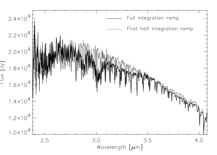
Figure 1: The final band 1 spectra of $\alpha$ Orionis : either based on uncorrected data (black) or on data corrected for presaturation (grey). The spurious spectral feature around $3.0\mu$m has disappeared.

A comparison between the 2 spectra, the original one and a corrected one, after reduction, is shown in Fig. 1: the spurious spectral feature around $3.0\mu$m has disappeared.

Memory effects

Band 2 (Si:Ga detectors, $4.08-12$ $\mu$m) is notoriously sensitive to memory effects, especially for sources with a flux above 1000 Jy such as $\alpha$ Orionis (Kester et al., 2001). The detector ’remembers’ a previous illumination and therefore predicts too large a flux for the current observation. Since each sub band is scanned both from short to long wavelengths and vice versa, it is possible to estimate the strength of the memory effects. Fig. 2 shows up scan, down scan and final version of the $\alpha$ Orionis spectrum. Strong memory effects are indeed present. We must therefore keep in mind that the correction may not be flawless from 4.08 to 4.3 $\mu$m and between 4.8 and 5.5 $\mu$m.

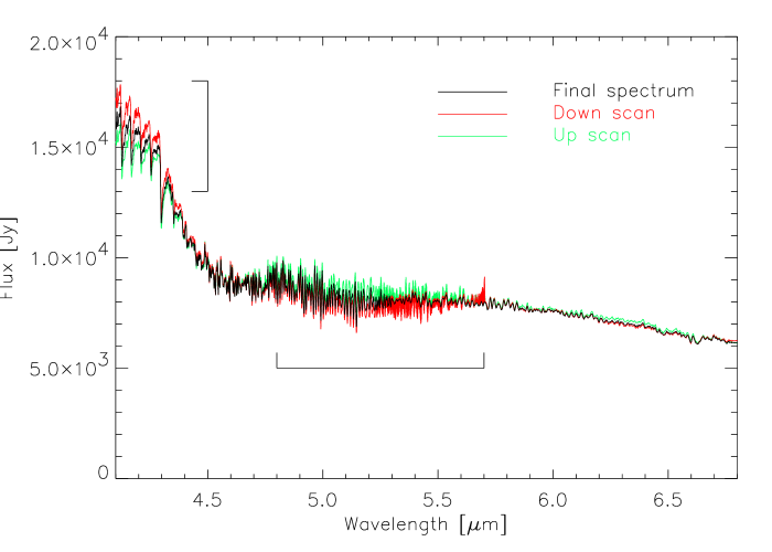
Figure 2: Up scan (green), down scan (red) and final spectrum (black) in band 2a and 2b. Memory effects are strong at the blue side and at 5.4 $\mu$m. The final flux may not be estimated correctly from 4.08 to 4.3 $\mu$m and between 4.8 and 5.5 $\mu$m. We keep this in mind when comparing to the models.

Absolute calibration

Another peculiarity of the reduction of this observation concerns the multiplicative factors we use to paste the different sub bands together. The general strategy is the following: band 1d ($3.02-3.52\leavevmode\nobreak\ \mu$m) is believed to have the best absolute flux calibration. Using the overlap between the different sub bands, it is then possible to shift the other bands to the correct level, starting from those adjacent to 1d and moving band-by-band to the red and blue. Usually the factors used are quite close to unity, with differences up to a few percent. However, for the spectrum of $\alpha$ Orionis, several factors differ significantly from unity. We remark that scaling factors closer to unity would be possible if we assume the absolute calibration of band 1d to be too low (see Sect. 4.3). Also the memory effects at 4.1 $\mu$m could influence the scaling factor of band 2a by 5%. For completeness, we list these scaling factors in Table 1.

Table 1: Multiplicative factors used to scale the different sub bands of the $\alpha$ Orionis spectrum to the absolute flux level when the latter is either determined by the flux level in band 1d (3rd column) or by requiring the average of the scaling factors to be equal to 1 (4th column). The large deviations from unity in the 1d-referenced scaling suggest that the absolute flux in band 1d might be underestimated. Further evidence supporting this hypothesis is given in Sect. 4.3. The large jumps between some bands can be (partially) attributed to the use of three different filters and apertures and 4 different detector types.

Band	$\lambda$ [$\mu$m]	1d	mean$=$1
1a	$2.38-2.60$	0.97	1.15
1b	$2.60-3.02$	0.98	1.16
1d	$3.02-3.52$	1.00	1.19
1e	$3.52-4.08$	0.97	1.15
2a	$4.08-5.30$	0.78	0.93
2b	$5.30-7.00$	0.80	0.95
2c	$7.00-12.0$	0.66	0.79
3a	$12.0-16.5$	0.71	0.84
3c	$16.5-19.5$	0.75	0.89
3d	$19.5-27.5$	0.76	0.90

2.2 Interferometry

Literature data

$\alpha$ Orionis has been studied extensively with interferometric techniques in the Near- and Mid-IR. In this work, we use 3 sets of IR observations that were already published: (1) broad band FLUOR observations at 2.2 $\mu$m first presented in Perrin et al. (2004a), (2) TISIS L band observations at 3.8 $\mu$m (Chagnon et al., 2002) and (3) ISI narrow-band Mid-IR observations at 11.15 $\mu$m (Weiner et al., 2003).

The K band data cover molecular bands of H₂O and CO, the L band data those of H₂O and SiO. These molecules may very well be present in the molsphere around $\alpha$ Orionis. We note that, if the extra molecular layers are optically thin, both bandpasses remain photosphere-dominated and are therefore well suited for our analysis.

The mid-IR visibilities not only sample the photosphere+molecular layers, but also the dust shell which emits strongly at 11 $\mu$m. In the case of $\alpha$ Orionis, the silicate emission of the dust shell originates in a region far from the central object: the inner radius, R_in, is believed to be 0.5 arcsecond (Sloan et al., 1993) or even 1 arcsecond on the sky (Danchi et al., 1994), to be compared to 22 mas for the photospheric radius (Perrin et al., 2004a). The silicate emission is therefore totally resolved at the spatial frequencies of interest for the study of the central object. If one knows the flux ratio $f=\frac{F_{star}}{F_{dust}}$, it is possible to renormalize the observed visibilities allowing an independent study of the central object without any other information on the dust shell. For $\alpha$ Orionis, this flux ratio at 11.15 $\mu$m is well-determined through other ISI observations (Danchi et al., 1994; Bester et al., 1996; Sudol et al., 1999) at very low spatial frequencies which sample the visibility curve at the point where the dust shell is being resolved. The derived values for the flux ratio $f$ range from 55 to 65 percent.

New data

$\alpha$ Orionis was observed in the N-band with the Mid-IR interferometric instrument MIDI (e.g. Leinert et al., 2003) on the VLT-I (e.g. Glindemann et al., 2000) in Science Demonstration Time (SDT) on November 8 and 10, 2003. The interferometric data will be presented and analysed in a forthcoming paper, together with additional MIDI observations scheduled for autumn 2005 which will cover a wider range in spatial frequencies.

MIDI single-dish spectra

As shown in Chesneau et al. (2005), it is also possible to obtain good quality N-band spectra from MIDI observations: for calibration purposes, single-dish spectra are observed with both UT telescopes separately just prior or after the interferometric observations. We searched these spectrally dispersed 1-D images (0.54 arcsec wide slit) for extended emission from the detached dust shell but found none. Spectra were constructed by integrating the images in the spatial direction with or without mask, which did not yield significant changes in spectral shape. We use here the spectra constructed with mask because of their higher S/N. They were calibrated using the MIDI spectra of calibrator stars (HD 39400, K1.5IIb and 17 Mon, K4III) observed in between the Betelgeuse observations. The final averaged spectrum is shown in Fig. 9.

3 The modelling

The aim of this investigation is to simultaneously model IR spectroscopic and interferometric data in order to get a better understanding of the physical processes at work between photosphere and dust shell. Since we expect both the extended atmosphere and the dust shell to be optically thin, it is crucial that we treat every source of radiation properly. We can for example not neglect the strong molecular bands already present in the photospheric spectrum of a late-type supergiant: clearly not all molecular features seen in the IR originate in “extra” molecular layers.

Hydrodynamical models of oxygen-rich late-type stars are not yet in a stage where they can provide an accurate reproduction of observations, and the general consensus is that we are still missing some fundamental knowledge on the major processes, such as the dust condensation sequence (e.g. Tielens, 1990). Moreover, these models are currently built only for low-mass (Mira and C) stars, and their applicability to supergiants is not clear. Therefore, we choose not to use such a self-consistent model, but instead construct a semi-empirical model as described below.

We will divide our model into 3 parts: (1) the hydrostatic photosphere, (2) a region of extra molecular layers and (3) the dust shell. The approximation of the extended atmosphere, i.e. the part containing the extra molecular layers, with a discrete instead of a continuous density, temperature and composition distribution is supported by the first generation of hydrodynamical models for AGB stars which predicts these distributions to be strongly radially peaked (e.g. Woitke et al., 1999; Höfner et al., 2003).

For each part, we have used the most up-to-date models available. They are described below.

3.1 The photosphere

To model the photosphere of this supergiant, we use the sosmarcs code, version May 1998, as developed by Gustafsson et al. (1975); Plez et al. (1992, 1993) at the university of Upssala, Sweden. This code is specifically developed for the modelling of cool evolved stars, i.e. a lot of effort was put into the molecular opacities, and they allow for the computation of radiative transfer in a spherical geometry. The line lists —relevant for the IR part of the spectrum— used are those of Goldman et al. (1998) for OH, Goorvitch (1994) for CO, Langhoff & Bauschlicher (1993) for SiO and those of Partridge & Schwenke (1997) for H₂O. This code solves the radiative transfer equation in a hydrostatic LTE environment with an ALI method (e.g. Nordlund, 1984). Opacities are treated with the opacity sampling (OS) technique at 153910 wavelength points, which guarantees a good sampling of both molecular and continuum opacity sources. This OS grid offers a good compromise between computational speed and accuracy of the atmospheric structure of the model. In the interpretation of the similarities and discrepancies between observed and synthetic spectrum, we make use of the study of the influence of the stellar parameters on a synthetic spectrum performed by Decin (2000). The initial values of the model parameters (which are T_eff, $\log{g}$, mass, the abundances of C, N, and O, the microturbulent velocity, $\xi_{\rm{t}}$ and the metallicity [Fe/H]) were determined in great detail for $\alpha$ Orionis by Lambert et al. (1984). They are listed in Table 2.

Table 2: The stellar/atmospheric parameters of $\alpha$ Orionis, according to Lambert et al. (1984), for a temperature of 3800 K (their own estimate) and for a temperature of 3600 K (as suggested by other temperature determinations).

parameter	value	value
$\rm{T}_{\rm{eff}}$	3800 K	3600 K
$\log{g}$	0.0	0.0
Mass	15 M⊙	15 M⊙
$\epsilon(\rm{C})$	$8.41$	$8.29$
$\epsilon(\rm{N})$	$8.62$	$8.37$
$\epsilon(\rm{O})$	$8.77$	$8.52$
$\xi_{\rm{t}}$	4 km/s	4 km/s
$[\rm{Fe}/\rm{H}]$	0.00	0.00

For $\alpha$ Orionis, masses derived from theoretical Hertzsprung-Russell diagrams range from 15 M_⊙ (Lamb et al., 1976; Cloutman & Whitaker, 1980) to 30 M_⊙ (Stothers & Chin, 1979). Adopting a distance of 131 parsec (Hipparcos, Perryman et al., 1997) and a photospheric angular diameter of 43 mas yields a stellar radius of about 645 R_⊙. This result confirms the value for the gravity found by Lambert et al. (1984), derived from the fact that neutral and ionized lines should yield the same abundances. We stress the quality of this determination of the surface gravity because photospheric molecular bands, and especially those of water, are highly sensitive to the surface gravity (Decin, 2000).

The molecules responsible for absorption in the ISO-SWS wavelength region are primarily CO, H₂O, OH and SiO. The contribution of these molecules to the total absorption, when adopting the stellar parameters of Lambert et al. (1984), is shown in Fig. 3.

Figure 3: Main contributions to the total photospheric absorption in the atmosphere model with the stellar parameters from Lambert et al. (1984) at 3600 K. CO and SiO are clearly dominant, while there are only minor traces of absorption by water. The relevant line lists used are those of Goldman et al. (1998) for OH, Goorvitch (1994) for CO, Langhoff & Bauschlicher (1993) for SiO and those of Ames (Partridge & Schwenke, 1997) for H₂O.

3.2 The molecular layers

Several approaches are possible when modelling molspheres. They range from plane-parallel slabs placed in front of the star (e.g. Yamamura et al., 1999; Matsuura et al., 2002; Cami, 2002; Van Malderen, 2003) over infinitesimally thin spherical shells (Perrin et al., 2004b) to extended spherical layers with temperature and density distributions (Mennesson et al., 2002; Ohnaka, 2004a, b).

Slab models are not suitable for our purposes: the molecular layers are expected to be fairly optically thin, in which case the slab-approximation is far too rough (in a first order because these models do not take into account that the visible column density is twice as high next to the stellar disk as it is in front of it, and to a second order because they miss sphericity effects which are important for large scale heights). Both the resulting spectra and the resulting visibilities are therefore not realistic for optically thin molspheres.

On the other hand, the shocked nature of these layers most probably implies that they are geometrically quite thin and that therefore temperature and density gradients within the shell can be neglected. Moreover, the observational data are at the moment too limited (in both spectral and spatial resolution) to constrain these supplementary parameters.

Consequently, we opt for isothermal, spherical layers with a finite extent but no density distribution, which are characterized by their temperature, composition, column density for each molecule, inner radius and outer radius. Fig. 4 visualizes the structure of the models used.

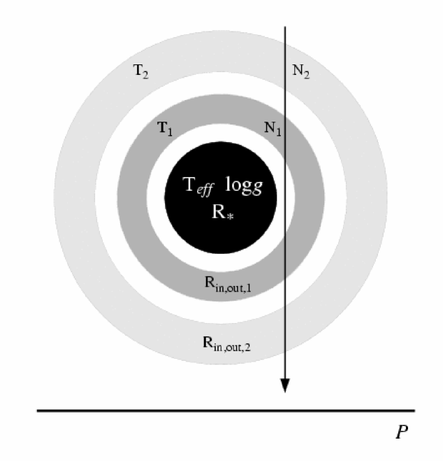
Figure 4: The structure of the models presented here: a photospheric model which includes limb darkening and the relevant molecular opacity, surrounded by layers of possibly mixed composition, each with its temperature, density, inner radius and outer radius. For the silicate feature modelling, the resulting spectrum is fed into the dust radiative transfer code modust (Bouwman et al., 2000).

3.2.1 Opacities

Opacities were calculated for H₂O, SiO, CO, and OH at temperatures ranging from 500 to 2500 K, with 100 K increments.

For H₂O, we used the nasa ames line list and partition function (Partridge & Schwenke, 1997), which is at present the most complete list, including more than 300 million lines. However, for computational reasons, we included only lines with $\log{gf-\chi\theta}\geq-9$, with $g$ the ground level statistical weight, $f$ the oscillator strength, $\theta=5040/3500$ and $\chi$ the excitation energy in eV. The consequences of neglecting the weaker lines on the final opacity are below 1 percent for a spectral resolution of 300 (Van Malderen et al., 2004). Differences between the available line lists for H₂O (e.g. ames, hitemp, scan) are significant. The hitemp line list is aimed at temperatures of about 1000 K, and might not be valid for the very high temperatures of the water around Betelgeuse. Decin et al. (2003) found the best reproduction of observed water spectra in the ISO-SWS spectra of M giants with the ames line list, for which reason we used it here as well.

CO, OH and SiO present far less difficulties than water. We used the line list of Goorvitch (1994), Goldman et al. (1998) and Langhoff & Bauschlicher (1993) respectively. These are the most complete lists to date for astrophysical applications (Decin, 2000). The polynomial expansion of the appropriate partition function was taken from Sauval & Tatum (1984).

As microturbulent velocity we use 3 km s^-1 as suggested for cool giants by Aringer et al. (2002).

3.2.2 Radiative transfer

We compute emerging intensities for a grid of linearly spaced impact parameters $p$ (256 in total), i.e, we construct a 1-D intensity profile $I(\lambda,p)$, going from the center of the disk to the edge. From this intensity profile, both the resulting spectrum and the visibilities can be calculated. For more details on the calculation of the radiative transfer, we refer to Verhoelst (2005).

An example of such an intensity profile for a single layer around a limb-darkened central star is shown in Fig. 5.

Figure 5: An example of an intensity profile at 2.9 $\mu$m for our marcs photosphere, surrounded by a single layer with R${}_{\rm{in}}=1.35\rm{R}_{\star}$, R${}_{\rm{out}}=1.85\rm{R}_{\star}$, a temperature of 2300 K and a H₂O column density of $5\times 10^{20}$ cm^-2. The dip in the IP at $\sim 1$ R_⋆ is an artefact due to the assumption that the central star is optically thick also in the limb.

From the theoretical wavelength-dependent intensity profile, we calculate the spectrum by integration over the emitting surface and the monochromatic visibility by a Hankel transform (Hanbury Brown et al., 1974) of the intensity profile. This monochromatic visibility is then convolved with the bandpass of the observations for the comparison model vs. observations. For wide-band data close to and beyond the first null, bandwidth effects become important: because of the wavelength dependence of the spatial frequency at which we observe, one wide band visibility measurement actually covers a range in spatial frequencies, but is assigned to the spatial frequency corresponding to the effective wavelength of the filter. We follow the approach of Perrin et al. (2004a) and take this effect into account by averaging properly weighted squared visibilities.

3.3 The dust shell

The dust shell is modelled using the proprietary spherical radiative transfer code modust
(Bouwman et al., 2000; Bouwman, 2001). Under the constraint of radiative equilibrium, this code solves the monochromatic radiative transfer equation from UV/optical to millimetre wavelengths using a Feautrier type solution method (Feautrier, 1964; Mihalas, 1978). The code allows to have several different dust components of various grain sizes and shapes.

4 Comparison with observations

When confronting the synthetic spectrum based on our marcs model atmosphere with the ISO-SWS spectrum of $\alpha$ Orionis (Fig. 6), it is clear that our model makes a good reproduction of the global spectral shape. This shape is quite different from that of a blackbody: clearly, the major sources of opacity have a strong influence on the spectral appearance in the IR, which is well reproduced by the marcs model atmosphere. However, several differences can be observed:

• between 2.38 and 3.5 $\mu$m the model strongly overestimates the flux,

• from 4.0 to 4.2 $\mu$m the flux is underestimated,

• around 5 $\mu$m, there are extra absorption features in the ISO-SWS spectrum,

• also from 6 $\mu$m onward there is extra absorption, and

• from 8.5 $\mu$m on-wards, the observed spectrum is dominated by silicate emission.

The latter property clearly divides the spectrum in a part without dust contribution, and a part which will require a modelling of the dusty outflow. We are therefore motivated to separate at first the analysis of the near-IR part of the spectrum from that of the mid- to far-IR wavelength regime.

4.1 The near IR

We start with a study of the near-IR wavelength regime, where photospheric emission dominates, but several discrepancies require further investigation, as noted above.

4.1.1 Comparing marcs with ISO-SWS

Unfortunately, the first three discrepancies coincide with wavelength regions not free of calibration problems: the first one corresponds to that affected by presaturation. We are however confident that this issue was dealt with in an appropriate way as discussed in Sect. 2.1, and that the discrepancy seen is of a physical nature. As to the 2nd region: this is the blue side of band 2a, which shows strong memory effects as shown in Sect. 2.1 and Fig. 2. The same is true for the 3rd region, but the discrepancy is much wider than the wavelength band affected by memory effects (cf. Fig. 2). Since a correction for memory effects was applied, we can at this point not rule out the possibility that these are also true discrepancies between model and reality.

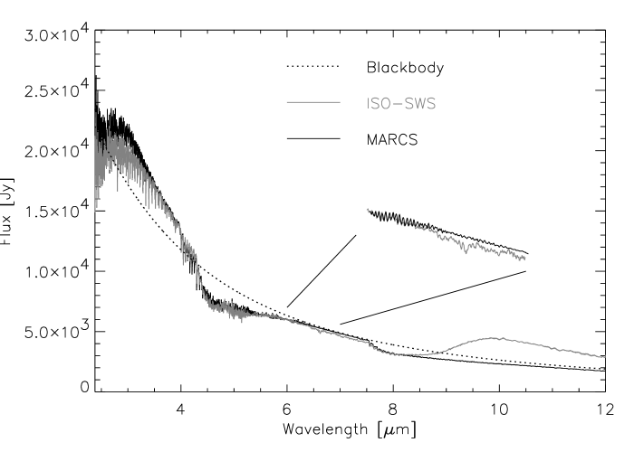
Figure 6: A comparison between the ISO-SWS-spectrum (grey) and our synthetic marcs spectrum (black). A blackbody at T=3600 K is shown by the dotted line for comparison. Clearly, our model can reproduce the global spectral shape very well. Nevertheless, there are some interesting discrepancies.

From Fig. 3 and 6, it is clear that the first and fourth discrepancy, i.e. the strongest ones, can be due to unpredicted absorption by water, while the second one appears to correspond to SiO. Some contribution of extra CO absorption might also be present in the 2.38 and 5 $\mu$m discrepancies.

However, for the parameters being studied, the model predicts almost no absorption by water: the atmospheric temperature is too high, except for the outermost layers. Lowering the effective temperature is not an option, because it is well constrained by the apparent diameter and the bolometric flux (e.g. Perrin et al., 2004a). Using a higher oxygen abundance does not work either since a very large increase would be required, which then causes far too strong spectral features by OH and SiO. Also an attempt at increasing the H₂O absorption with a higher surface gravity fails: a physically impossible value of $\log{g}=2$ would be required (see Sect. 3.1 for a discussion on the determination of the gravity).

Concerning the excess emission by SiO at 4.2 $\mu$m: since the SiO band at 8 $\mu$m is well predicted by the model, it is most likely only a memory effect and therefore not real.

We conclude that we see clear extra absorption by H₂O which cannot be predicted by the hydrostatic marcs model with reasonable input parameters. The problem thus appears not to be in the input parameters but in the basic assumptions. Three of these are not very likely to hold in the atmosphere of a variable supergiant: LTE, homogeneity and hydrostatic equilibrium.

LTE is most definitely violated in the outermost layers of the photosphere where the density is low (see e.g. Ryde et al., 2002). However, non-LTE effects are generally only seen in high-resolution spectra (e.g. Ayres & Wiedemann, 1989), and are not believed to create pseudo-continuous effects such as seen here in $\alpha$ Orionis.

The second assumption, homogeneity, is probably also violated in the atmosphere of Betelgeuse. Freytag et al. (2002) calculated convection models for Betelgeuse and found large convective cells with strong temperature gradients between the border regions and the center. Possibly, more molecules, including H₂O, could form there too.

The last assumption has been well studied in the context of Mira stars. Hydrodynamic models are essential in the modelling of observed IR spectra of these pulsators (Woitke et al., 1999; Höfner et al., 2003). Although the amplitude of the visual variations of $\alpha$ Orionis is small compared to that of a typical Mira, i.e. about 0.25 mag in V (Gray, 2000) vs. 3 mag for e.g. T Cep (Van Malderen, 2003), the low surface gravity and high luminosity may help the levitation of the upper layers. As for Mira stars, the temperatures in this levitated matter can be low enough for molecules to form. If shocks are formed, by outward moving material running into infalling material, high molecular density shells will result.

Extra molecular layers are thus an attractive solution for the observed discrepancies. We will investigate this hypothesis below, but let us first remark that the angular diameter on the sky required to fit the ISO-SWS spectrum is only 43.6 mas (limb-darkened diameter of the $\tau_{\rm{ross}=10^{-7}}$ layer), to be compared to an observed LD diameter of 45.6 mas (obtained by fitting L band visibilities computed from our marcs model to the TISIS observations). This confirms the hypothesis formulated in Sect. 2.1 that the absolute calibration of the ISO-SWS spectrum based on band 1d has caused an underestimation of the actual flux, resulting in both the large deviations from unity for the scaling factors presented in Table 1 and the discrepancy in photometric and interferometric diameter reported here. The interferometric diameter would suggest the actual flux to be about 10% higher than predicted by band 1d (cfr. Table 1).

4.1.2 Adding an H₂O layer

Fitting the ISO-SWS spectrum with a photosphere+water-layer model, by a $\chi^{2}$ minimization in the grid presented in Table 3, we find the best fit for a layer of 1750 K, with an outer radius of 1.45 R_⋆ and an H₂O column density of $2\times 10^{19}$ cm^-2.

A few discrepancies remain, and they can be identified as due to CO (at 2.4 and 4.5 $\mu$m) and OH (several strong lines between 3 and 3.5 $\mu$m). The fit to the ISO-SWS spectrum can be improved some more by adding $2\times 10^{21}$ cm^-2 of CO and $5\times 10^{20}$ cm^-2 of OH. The resulting synthetic spectrum is shown in Fig. 7.

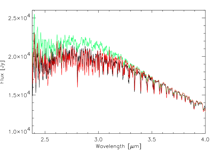
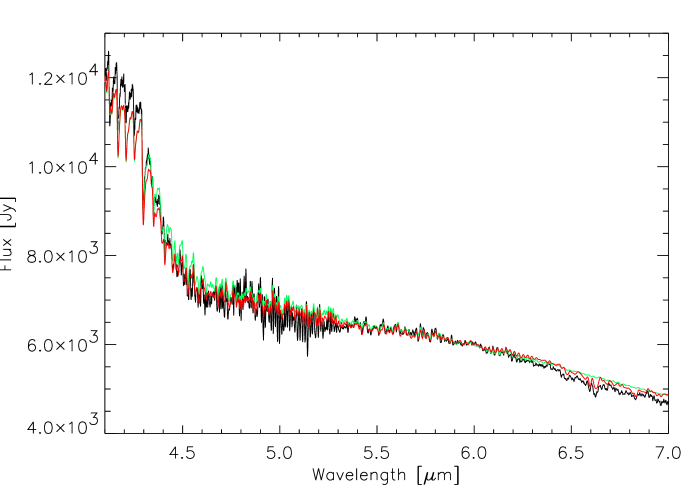
Figure 7: The ISO-SWS spectrum (black) is compared to the marcs photosphere model (green), and the marcs photosphere model embedded in a molecular layer (red) at 1.45 R_⋆, with a temperature of 1750 K and H₂O, CO and OH column densities of $2\times 10^{19}$ cm^-2, $2\times 10^{21}$ cm^-2, and $5\times 10^{20}$ cm^-2 respectively. The improvement is significant. The problems at 4.2 and 5 $\mu$m can be attributed to memory effects in the ISO-SWS observation (see Fig. 2).

Table 3: The grid of layer parameters in which we search for a best fit to both the ISO-SWS spectrum and the interferometric data.

parameter	min. val.	max. val.	stepsize
Rout [R⋆]	1.20	1.50	0.05
Temp. [K]	1500	2500	100
Col. dens. H2O [cm-2]	$6\times 10^{18}$	$4\times 10^{20}$	$\times$ 2
Col. dens. CO [cm-2]	$1\times 10^{20}$	$1\times 10^{24}$	$\times$ 10
Col. dens. OH [cm-2]	$1\times 10^{20}$	$1\times 10^{24}$	$\times$ 10
Col. dens. SiO [cm-2]	$1\times 10^{20}$	$1\times 10^{24}$	$\times$ 10

4.1.3 Comparison with the near-IR interferometric data

From this model, we can compute K and L wide band visibilities, to be compared to the FLUOR (K) and TISIS (L) observations. The result is shown in Fig. 8. The agreement is convincing for a photospheric limb-darkened diameter of 45.6 mas. In fact, the layer opacity in the FLUOR and TISIS bandpasses is so low that there is no noticeable difference in visibility curve between pure photosphere and photosphere+layer model.

Figure 8: Observed K and L band visibilities are compared to our best single layer model. The match is excellent for a photospheric LD diameter of 45.6 mas. The very discrepant points at low spatial frequency are TISIS L band observations, which might be corrupted by a poor subtraction of the thermal background.

The derived photospheric diameter is slightly larger than determined from the same data by Perrin et al. (2004a), but this is due to the extent of our stellar photosphere model: the outermost layer of our model corresponds to R${}_{\tau_{\rm{ross}}=10^{-7}}$. This translates into a “tail” on the intensity profile which is not present in the analytical profile used by Perrin et al. (2004a) and which amounts to about 4 percent of the total stellar diameter. We conclude that the photospheric diameter of our best-fitting photosphere+layer model is in good agreement with the one found by Perrin et al. (2004a), i.e. that the molecular layer does not change the apparent size in the near-IR at low spectral resolution.

4.2 The mid IR

4.2.1 Excess emission and a larger apparent diameter

The mid-IR part of the ISO-SWS spectrum is dominated by the Si-O stretching and O-Si-O bending resonances in amorphous olivines at 9.7 and 18 $\mu$m respectively (Fig. 10). The MIDI N-band spectra on the other hand do not show such a 9.7 $\mu$m feature (Fig. 9). The slit used for the latter observations is only 0.52 arcsec wide. This confirms the large inner radius of the olivine dust shell as suggested by Sloan et al. (1993) who found no silicate emission inside a region of about 0.5 arcsec, some emission between 0.5 and 1 arcsec, and the better part of the silicate emission even further out. This is also consistent with UKIRT mid-IR images presented by Skinner et al. (1997) and with the inner radius (1 arcsec) measured by Danchi et al. (1994) with the ISI interferometer.

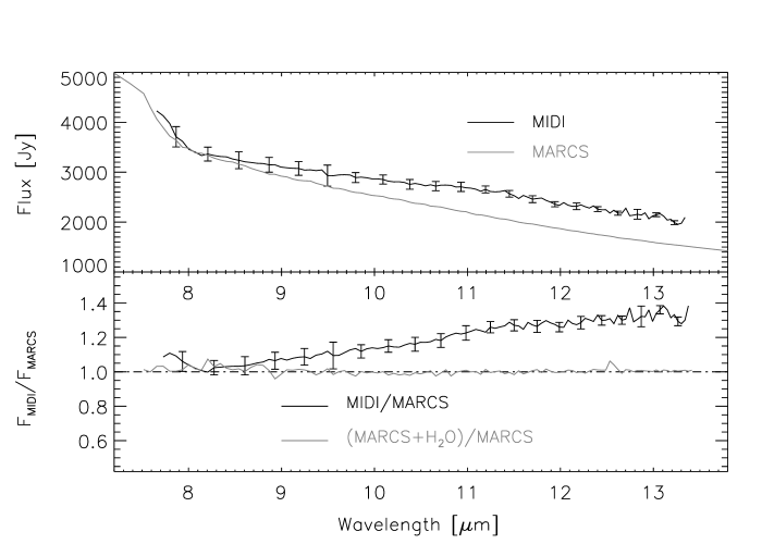
Figure 9: Average MIDI N-band spectrum compared to the marcs prediction for the photospheric emission. Upper panel: the calibrated MIDI spectrum and the marcs photospheric spectrum. There is no trace of olivine emission in the MIDI slit, which is 0.54 arcsec wide, confirming that the olivine dust is indeed more than 10 R_⋆ out. Lower panel: the MIDI spectrum divided by the marcs spectrum. There is excess emission within the PSF which increases with wavelength up to about $11-12$ $\mu$m and then levels out.

Surprisingly, there is excess (non-silicate) emission within the PSF of the MIDI N-band spectra which increases with wavelength up to about 11 $\mu$m and then levels out (Fig. 9). That such excess emission is present is also confirmed by a modust modelling of the dust shell based on the ISO-SWS spectrum: in Fig. 10, we see that the 2 features due to amorphous olivine can be modelled quite accurately but that the flux predicted in between is far too low. This problem cannot be solved with other grain sizes, nor with another extent of the dust shell. However, when subtracting the excess emission seen in the MIDI spectrum from the ISO-SWS spectrum, we arrive at a far better agreement between model and observations. Moreover, the excess seems to decrease again beyond 13 $\mu$m, disappearing entirely at 17 $\mu$m.

Table 4: Dust shell parameters for the best fit to the ISO-SWS spectrum. The dust shell inner radius corresponds to the measured inner radius of Skinner et al. (1997) and Sloan et al. (1993). The dust to gas ratio is taken from Knapp et al. (1980) and the outflow velocity from Knapp & Morris (1985). Grain shapes are a continuous distribution of ellipsoids (CDE).

Parameter	Value
$\dot{\rm{M}}_{\rm{dust}}$	$6.3\times 10^{-10}$ M⊙ yr-1
v∞	15 km s-1
Dust to gas ratio	0.0025
Rin	20 R⋆
Rout	$\infty$
Composition	Amorphous MgFeSiO4
Grain size	$0.01-1$ $\mu$m
Grain shapes	CDE

We remark that the dust mass loss rate we derive from a best fit to the ISO-SWS spectrum ($6.3\times 10^{-10}$ M_⊙ yr^-1) is in good agreement with that found by Knapp et al. (1980), Knapp & Morris (1985), Knapp (1986) and Skinner & Whitmore (1987). It is worth stressing that in the case of this optically thin dust shell, it is important to take into account the photospheric SiO band head at 8 $\mu$m when using the 9.7 $\mu$m feature to determine the dust mass loss rate.

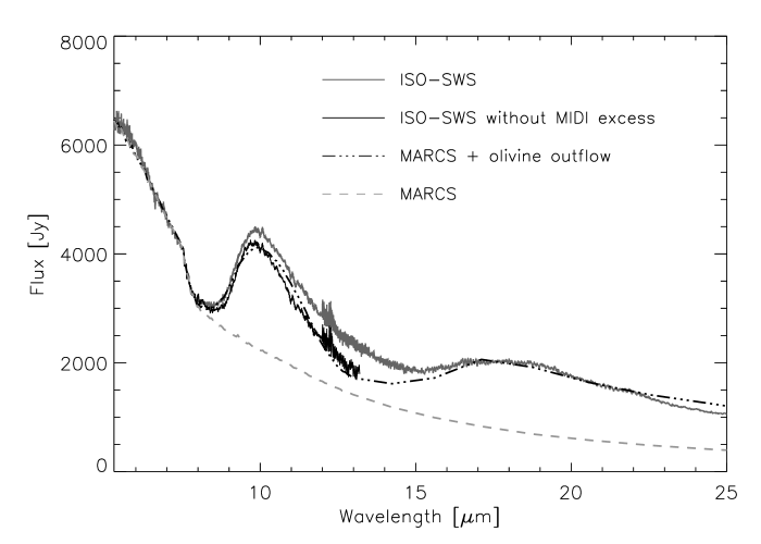
Figure 10: The ISO-SWS spectrum of $\alpha$ Orionis (black) in the mid-IR is dominated by the amorphous olivine resonances at 9.7 and 18 $\mu$m respectively. If the dust features are modeled with an olivine outflow (parameters listed in Table 4), a large discrepancy from $8-17$ $\mu$m suggests another source of emission/opacity. Indeed, when we subtract from the ISO-SWS spectrum the excess emission found in the MIDI N-band spectrum, the agreement is far better (solid line).

Weiner et al. (2003) present ISI observations (at 11.15 $\mu$m) performed between November 1999 and December 2001 at spatial frequencies which cover very well the first lobe of the visibility curve due to the central object, i.e. the object inside e.g. the MIDI PSF. Together with earlier observations at much smaller baselines which allow the determination of flux ratio between central object and olivine dust shell, these allow a diameter determination of the central object at that wavelength. The flux ratio determined from these observations ranges from $55-65$ percent (Danchi et al., 1994; Bester et al., 1996; Sudol et al., 1999) which is compatible with the flux from the central object in the MIDI spectra. The diameter is about $55-60$ mas (Weiner et al., 2003), i.e. almost 1.5 times the size in the near IR. Moreover, no data in the second lobe of the visibility curve are available, and limb-darkening may therefore be significant, increasing the size of the central object at 11.15 $\mu$m even more.

4.2.2 Explaining the mid-IR data

In the previous section, we found that in the mid IR, $\alpha$ Orionis (without the detached olivine dust shell) appears to be about 1.5 times as large as in the near IR. Moreover, we found excess emission from 8.5 $\mu$m onward, which increases smoothly with wavelength up to about 11 or 12 $\mu$m, where the excess levels out at $25-30$ percent. Beyond 17 $\mu$m there appears to be no longer an excess. There are 3 possible sources of extra opacity which could be responsible for the observed excess and diameter increase: (1) an extra molecular layer, (2) chromospheric emission and (3) dust. Below, we investigate each of these possibilities.

An extra molecular layer

From an analysis of the near-IR part of the ISO-SWS spectrum, we found evidence for an extra molecular layer at about 0.45 R_⋆ above the photosphere, containing mainly water. This putative layer is so optically thin that it does not influence the apparent size in the K and L bands. Since H₂O opacity is in fact even lower around 11 $\mu$m (e.g. Van Malderen, 2003), we do not expect a significant diameter increase at those wavelengths. Indeed, to reproduce the ISI observations, the layer has to contain about $2\times 10^{22}$ cm^-2 of water (upper panel of Fig. 11), which is 1000 times more than what we found from the near-IR part of the spectrum. Such a thick H₂O layer is clearly not present: it would create optically thick water bands in the near-IR as well, and those are not seen in the ISO-SWS spectrum. Moreover, H₂O opacity has a minimum around 10 $\mu$m which would yield a clear spectral signature in the MIDI N-band spectrum (unless the layer is extremely thick and isothermal), which is not observed. We conclude that H₂O opacity can not be responsible for the observed diameter increase and excess emission.

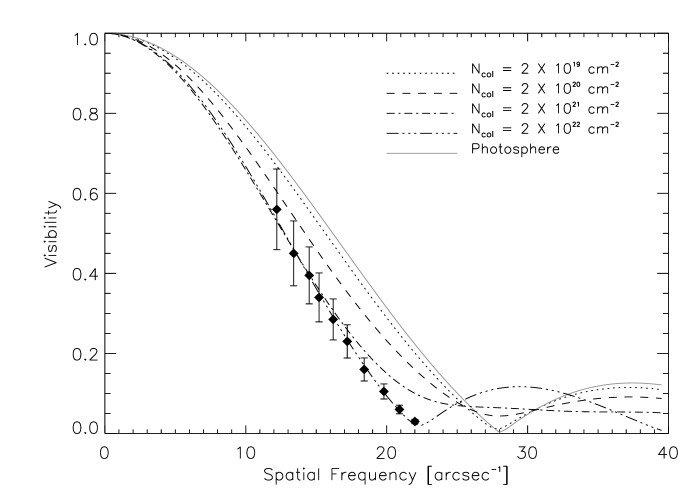
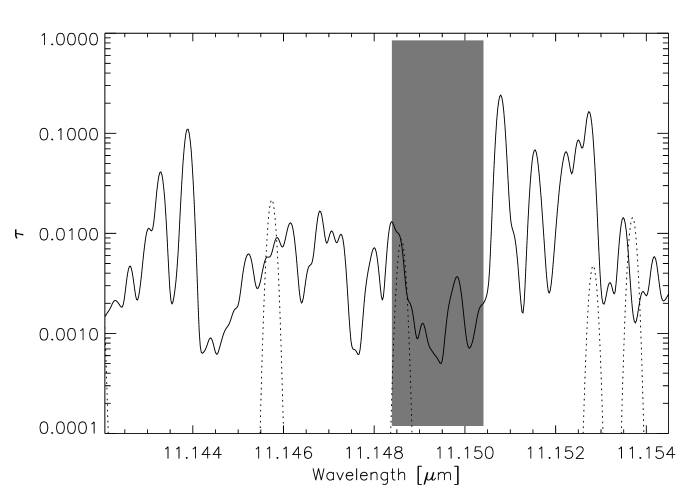
Figure 11: Upper panel: Comparison of different models with the ISI observations (diamonds) at 11.15 $\mu$m made by Weiner et al. (2003). To match these data with an H₂O layer, we need a high H₂O column density of about $2\times 10^{22}$ cm^-2, which is neither compatible with the near-IR spectrum, nor with the MIDI N-band spectrum. Lower panel: Opacity in the ISI bandpass (shaded region) of $2\times 10^{19}$ cm^-2 of H₂O (solid line) and $2\times 10^{21}$ cm^-2 of SiO (dotted line), both at a temperature of 1750 K. The opacity profile is redshifted by 21 km s^-1, which is the radial velocity of $\alpha$ Orionis (Wilson, 1953).

However, there may be other molecular sources of opacity at 11.15 $\mu$m. As can be seen from Fig. 3, both SiO and OH show spectral lines around 11 $\mu$m (TiO, which is not shown in Fig. 3, does not have significant lines in the mid-IR). Those of OH are well separated and not very numerous: our line list (Goldman et al., 1998) has no strong lines in the ISI bandpass. The red wing of the opacity profile of hot SiO might cover the ISI bandpass, but a very large column density would be required to reach the required amount of opacity. This is not compatible with the lack of an extra-photospheric SiO signature around 8 $\mu$m in the ISO-SWS spectrum. The lower panel of Fig. 11 displays the opacity of H₂O and SiO in the ISI bandpass. We thus exclude a molecular cause for the diameter increase and excess emission is.

Chromospheric emission

From UV and radio observations, $\alpha$ Orionis is known to have both a hot chromospheric component and an ionized wind with fairly low electron temperatures (e.g. Basri et al., 1981; Gilliland & Dupree, 1996; Skinner et al., 1997; Lim et al., 1998). Harper et al. (2001) present a model of the gas in the extended atmosphere of $\alpha$ Orionis from $1-10$ R_⋆, which matches the radio data up to the mid IR. It consists of a weakly ionized wind with mainly H^- f-f opacity. The temperature distribution peaks at about 80 mas (diameter) or 1.45 times the (mid-IR) ISI diameter. The maximum mean electron temperature in their model is only about 4000 K, but since that is not enough to explain the UV observations, they suggest an inhomogeneous medium: the region around 1.45 R_ISI has an ambient temperature of only 2000 K, but contains a multitude of chromospheric hot spots with electron temperatures of the order of 10000 K. With an areal filling factor (AF) of less than 0.25, this could reconcile the UV traces of a hot chromospheric component with a mean electron temperature of only 4000 K. While the mean model predicts neither excess emission nor a larger apparent size at 11.15 $\mu$m (Harper, private communication), we investigate whether the suggested chromospheric hot spots could be at the origin of the mid-IR excess and diameter increase.

We have strong constraints on the spectral shape of the excess emission and opacity: it should be transparent up to 8.5 $\mu$m, then increase strongly up to about 12 $\mu$m and decrease again toward longer wavelengths (Fig. 9 and 10). In the optically thin regime, the excess due to chromospheric emission is constant throughout the N band because the free–free opacity is proportional to $\lambda^{2}$ and the chromospheric temperature is high enough for the source function to be in the Rayleigh–Jeans limit. Such a constant excess is not compatible with the observed increase of the excess with wavelength (see also Fig. 13). In the optically thick regime, the observed shape of the excess requires (1) the temperature of the chromosphere to decrease strongly along the line of sight and (2) the opacity to reach unity within the N band. Because the total excess is far below that of a homogeneous, hot and optically thick chromosphere with a diameter of about 1.5 R_⋆, the chromosphere must be very clumpy.

To test this hypothesis, we constructed a model mimicking the central photospheric disk embedded in a halo with optically-thick chromospheric hot spots. This model yields the contrast ratio between the mean observed photospheric intensity and mean layer intensity as a function of layer diameter and chromospheric AF factor, under the constraint that the chromospheric hot spots must generate the excess emission seen at 11 $\mu$m in the MIDI spectrum and the visibilities observed with the ISI. Fig. 12 shows how each assumed diameter of the chromospheric layer requires a certain AF factor and hot spot temperature, if it is to match the observed excess and visibilities. The AF factor goes down asymptotically to zero for a layer radius approaching 1.8 R_⋆. At the same time, the chromospheric temperature increases to infinity, but it is clear that our model is too crude an approximation of the actual intensity distribution on the sky in this regime.

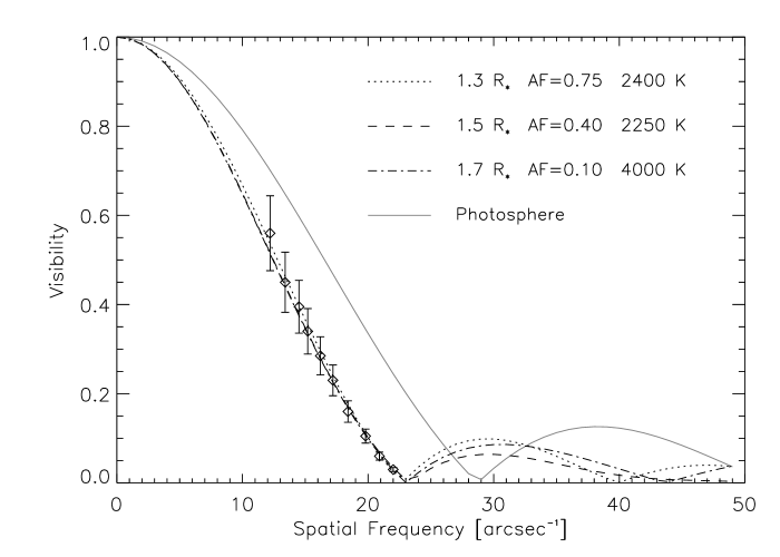
Figure 12: Both the visibilities and the excess emission at 11 $\mu$m can be explained as due to a halo covered with hot spots. Allowed layer diameters range from about 1.3 to 1.8 R_⋆. The derived hot spot temperatures remain well below the expected chromospheric temperature (10000 K, Harper et al., 2001).

We find that for almost the entire range of possible layer diameters, the hot spot temperature is far below the temperature of an actual hot chromospheric component (10000 K). Only in the asymptotic regime toward a layer radius of 1.8 R_⋆ (80 mas on the sky) does the model predict such a high temperature, at a very low AF factor (AF $\leq 0.03$), but the agreement with the observed visibilities is not as good as with a smaller layer diameter. Moreover, it appears unlikely that the very low AF factor can be combined with the requirements on the source function.

We conclude that, while there must be some emission by a hot chromospheric component in the mid IR, the hot spot temperatures and required areal filling factor, together with the spectral shape of chromospheric emission, appear to be in contradiction with the hypothesis that an inhomogeneous hot chromosphere is responsible for the observed N-band excess and diameter increase.

Dust

The last viable candidate source for the extra opacity and emission is dust. The maximum of the excess emission appears to be located close to 13 $\mu$m, which suggests a relation with the “13 $\mu$m feature” as seen in about 50 percent of all oxygen rich dust shells (Sloan et al., 1996) and attributed to a.o. Spinel (MgAlO₄, Posch et al., 1999), SiO₂ (Speck et al., 2000) or Alumina (Al₂O₃, Onaka et al., 1989). In fact, all but the last candidate have a fairly narrow, peaked absorption coefficient which can not explain our observations.

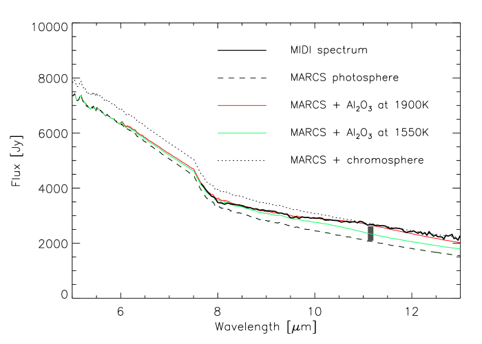
Figure 13: By including $1\times 10^{-3}$ g cm^-2 of amorphous Al₂O₃ at 1900 K in the layer at 1.45 R_⋆, we find a good fit to the ISI data (diamonds in the upper panel), and to the N-band excess (lower panel). The minor but systematic deviation at small spatial frequency suggests that the layer is actually located a little closer to the photosphere, i.e. 1.35 R_⋆. The grey box indicates the flux excess allowed by the flux ratio between the detached dust shell and the central object, i.e. the scaling factor used on the interferometric observations in the upper panel. The excess of an optically thin isothermal chromosphere as in Skinner & Whitmore (1987) is also shown (dotted line).

A simultaneous modelling of the N-band excess and the ISI visibilities with a layer of Al₂O₃ results in a very good agreement (Fig. 13) for a layer at 1900 K and a column density of $1\times 10^{-3}$ g cm^-2. Moreover, the transparency of Al₂O₃ in the near IR makes even the SiO band head at 7.7 $\mu$m well visible through the layer, as required by the ISO-SWS spectrum.

The derived temperature should be confronted with the temperature regime only 0.5 R_⋆ above the stellar photosphere. Although the effective temperature of $\alpha$ Orionis is 3600 K, the outermost layers of our marcs model have temperatures of the order of only 2000 K. It appears therefore not unlikely that the region 0.5 R_⋆ above the photosphere has a gas temperature of about 1900 K. However, demanding radiative equilibrium, i.e. the absorbed stellar radiation should be emitted thermally, we arrive at a much higher temperature, of the order of 2400 K.

Al₂O₃ dust grains are believed to condense in chemical equilibrium at a temperature of 1900 K only in high-pressure environments, i.e. for a total pressure above $10^{-2}$  bar (Lodders & Fegley, 1999). This required pressure is a factor of $10^{4}$ larger than the pressure in the outermost layers of our marcs photosphere.

Which one of the three?

A molecular origin can be ruled out right-away as long as we assume that there have not been drastic changes in the molecular environment of $\alpha$ Orionis between the epoch of the ISO-SWS and the near-IR interferometric observations and that of the mid-IR observations. The light curve of $\alpha$ Orionis (Fig. 14) shows no peculiar behaviour in that time span.

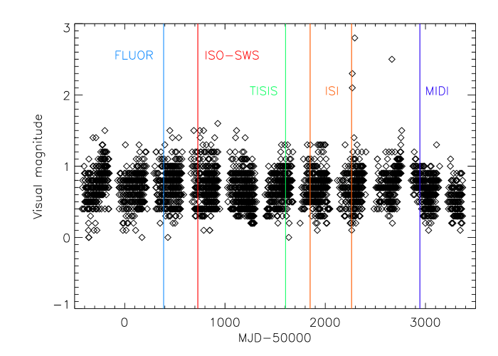
Figure 14: Light curve of $\alpha$ Orionis at the time of the observations presented in this paper. Constructed from observations by the American Association of Variable Star Observers (AAVSO) (Waagen, E. O. 2004, private communication)

Chromospheric emission is certainly present, and we cannot rule out some influence in the mid IR. However, as discussed above, we see no way of reconciling the spectral and spatial constraints with a chromospheric origin.

Dust appears to be the most attractive solution: it can reproduce spectral and spatial observations simultaneously. Nevertheless, the required temperature and pressure are a reason for concern. Furthermore, this inevitably leads to questions on the relation between such an Alumina layer and the detached olivine dust shell.

4.3 Discussion

The water layer

Let us start this discussion by returning to the near-IR observations. We found evidence for an optically thin molecular layer containing H₂O and maybe also CO and OH about 0.45 R_⋆ above the photosphere. The derived column density (about $2\times 10^{19}$ cm^-2) is slightly higher than that derived by Jennings & Sada (1998), but lower than that from Tsuji (2000b) and Ohnaka (2004b), as listed in Table 5. The lower value found by Jennings & Sada (1998) is the consequence of a higher adopted water temperature: $2500-2800$ K. However, this temperature is only an upper limit on the actual temperature of the H₂O (Jennings & Sada, 1998). Ohnaka (2004b) on the other hand infers both a higher temperature and a significantly larger column density. This is the consequence of his attempt to explain both the mid-IR water spectrum at 6 and 11 $\mu$m and the ISI diameter at 11.15 $\mu$m as being due solely to a layer of H₂O .

Table 5: Stellar and layer parameters for $\alpha$ Orionis, as derived by Jennings & Sada (1998), Tsuji (2000b), Ohnaka (2004b) and Perrin et al. (2004a). The first 2 determinations are purely spectroscopic, the third combines high-resolution spectroscopy and interferometry and the fourth one combines photometry with interferometry. (NA = not available)

Parameter	Jennings & Sada (1998)	Tsuji (2000b)	Ohnaka (2004b)	Perrin et al. (2004a)	This work
$\theta_{\star}$ [mas]	NA	NA	44.0	$42.00\pm 0.06$	45.6
T⋆ [K]	NA	3600	3600	$3690\pm 50$	3600
$\theta_{\rm{layer}}$ [mas]	NA	NA	$63.8\pm 6.4$	$55.78\pm 0.04$	65
Tlayer [K]	$\leq 2800$	$1500\pm 500$	$2050\pm 100$	$2055\pm 25$	1750
Layer Composition	H2O	H2O	H2O	undefined	H2O, Al2O3(?)
K, opacity	NA	NA	NA	$0.060\pm 0.003$	NA
L opacity	NA	NA	NA	$0.026\pm 0.002$	NA
11$\mu$m opacity	NA	NA	NA	$2.33\pm 0.23$	NA
H2O col. d. [cm-2]	$3\pm 2\times 10^{18}$	$\sim 1\times 10^{20}$	$1-4\times 10^{20}$	NA	$2\times 10^{19}$

Fig. 15 compares a model using the layer parameters of Ohnaka (2004b) with the ISO-SWS spectrum over the full wavelength range. Improvements w.r.t. the model as presented by Ohnaka (2004b) are the use of a marcs photosphere instead of a blackbody approximation and the use of the Ames line list for H₂O instead of that from the hitemp database. While this model reproduces quite well the spectral features between 6 and 7 $\mu$m also used by Ohnaka (2004b) (see inset of Fig. 15), it is not compatible with the spectro-photometric flux levels. Furthermore, the predicted band strength at 2.8 $\mu$m is too large and the SiO band head at 8 $\mu$m, clearly seen in the ISO-SWS spectrum, is no longer visible through such a thick layer. We conclude that the model as presented by Ohnaka (2004b) has too large an H₂O column density.

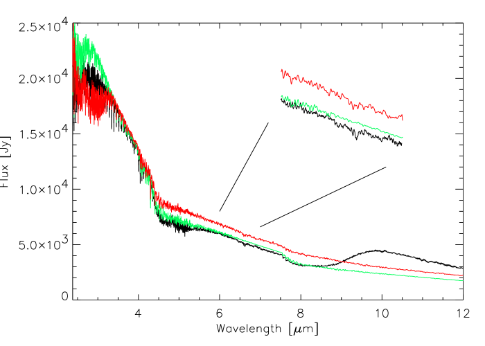
Figure 15: ISO-SWS spectrum (black), marcs photosphere model (green) and a photosphere+layer model (red) using the layer parameters by Ohnaka (2004b).

The dust layer

From the mid IR excess and the 11.15 $\mu$m interferometry, we found evidence for the presence of hot amorphous Al₂O₃ at about the same location above the photosphere as the H₂O layer. This is at least a factor of 10 closer to the star than the onset of silicate emission.

Several dust condensation scenarios ascribe a crucial role to Al₂O₃: it is assumed to be the first dust species to condense, and thereafter act as a seed nucleus for further dust condensation (e.g. Salpeter, 1977; Tielens, 1990; Sedlmayr, 1997; Lodders & Fegley, 1999). Remark that Patzer (2004) argue that this scenario is only valid in chemical equilibrium conditions, and therefore not in the rapidly expanding wind, but the conditions in the stationary layer we consider here may be more favourable to attain chemical equilibrium.

If indeed we have observed the very onset of dust formation, then it is quite puzzling why no dust is seen in between 1.5 and $10-20$ R_⋆. If the mass loss is not episodic, there are only two possibilities: either (1) there is no dust in this region, in which case it must be destroyed right after its formation, or (2) there is an outflow of amorphous Al₂O₃ but at such a low density and temperature that we do not see it.

The former scenario is plausible given the presence of a patchy hot chromospheric component which could destroy the Alumina before it reaches cooler regions. The dust seen at larger distances may well be formed anew, if the outflowing gas becomes again cool enough for condensation to occur. The silicate emission then does come from a detached shell.

The second hypothesis is supported by Onaka et al. (1989), who propose that the alumina grains are highly transparent up to the point where they collect silicates on their surface. Coupled with a very low density due to a strong acceleration at their birth in the molecular layer, this would make them invisible up to the silicate condensation location, where silicates settle onto the Al₂O₃ grains. We computed radiative equilibrium temperatures for both silicates and Al₂O₃ at the radius of the silicate condensation and find the Alumina to be cooler by a few hundred K, making it indeed undetectable!

This could mean that the dust shell of $\alpha$ Orionis is not really “detached” as previously assumed, but rather a continuous outflow from close to the stellar photosphere, which is transparent up to the point where silicates condense onto the alumina grains. Pure Al₂O₃ is then only visible at fairly high temperatures near the stellar surface where it is formed.

However, a major shortcoming in this scenario is that Alumina is fairly transparent at short wavelengths and therefore radiation pressure on a 0.01 $\mu$m grain is insufficient (by a factor of 10 at least) to initiate the outflow.

5 Conclusions and prospects

We have modelled the molecular (and possibly dusty) close environment of the late-type supergiant $\alpha$ Orionis. We took into account both spectral and spatial information from the near to mid-IR. The improvements over previous modelling attempts for $\alpha$ Orionis are the use of a sophisticated marcs model for the central star, the computation of radiative transfer through the molecular layers in spherical geometry, up-to-date line lists, and a larger set of observational constraints.

We find evidence for an optically thin layer of water close above the photosphere. This layer gives rise to some spectral signature, but does not increase the apparent size in the near-IR w.r.t. that of the pure photosphere. However, in the mid-IR, we find excess emission by amorphous silicates far out in the stellar wind (at least 20 R_⋆ from the stellar surface) and another source of excess emission much closer to the photosphere. The extra source of opacity close to the star is so optically thick that it increases the apparent size of the star with a factor of 1.5 from the near- to the mid-IR. It must however be fully transparent up to 8 $\mu$m, and the excess emission appears to decrease again beyond 15 $\mu$m. We show that it cannot be of a molecular origin since that would induce strong spectral features in the near IR. Chromospheric opacity/emission is most definitely present at radio and UV wavelengths, but we see no way to reconcile the spectral and spatial properties (inhomogeneity) of a chromosphere with the near and mid-IR observations. Dust grains of amorphous alumina (Al₂O₃) do yield a good spectral and spatial fit, but at an uncomfortably high temperature (1900 K). Nevertheless, this hypothesis fits in recent dust condensation scenarios and we believe it to be the most likely solution.

New MIDI observations at 5 different baselines, high spectral resolution and with simultaneous photometry are planned for autumn 2005 and, together with requested VISIR high spectral and spatial resolution observations in the Q-band, will undoubtedly help to select among the hypotheses.