The clumpiness of LBV winds

Abstract

We present the first systematic spectro-polarimetric study of Luminous Blue Variables (LBVs), and find that at least half those objects studied display evidence for intrinsic polarization – a signature of significant inhomogeneity at the base of the wind. Furthermore, multi-epoch observations reveal that the polarization is variable in both strength and position angle. This evidence points away from a simple axi-symmetric wind structure à la the B[e] supergiants, and instead suggests a wind consisting of localised density enhancements, or ‘clumps’. We show with an analytical model that, in order to produce the observed variability, the clumps must be large, produced at or below the photosphere, and ejected on timescales of days. More details of LBV wind-clumping will be determined through further analysis of the model and a polarimetric monitoring campaign.

¹School of Physics & Astronomy, University of Leeds, UK
²Blackett Laboratory, Imperial College, London, UK
³Astrophysics Group, Lennard-Jones Laboratories, Keele University, UK

1. Introduction

Luminous Blue Variables (LBVs, Humphreys & Davidson 1994, & Nota these proceedings) are very massive evolved stars that are found right at the top of the HR diagram, roughly the same region as the B[e] supergiants. Like the B[e]SGs, their spectra contain many emission lines due to their strong winds. Unlike the B[e]SGs, they are strongly photometrically variable, with amplitudes of 1-2 mags over timescales of a few months to years. The amount of material ejected by the LBVs is huge; their mass-loss rates are among the highest known ($10^{-5}-10^{-4}$M$\mbox{${}_{\normalsize\odot}$}\rm yr^{-1}$), whilst they can throw off many solar masses during giant eruptions (e.g. $\eta$ Car, Morris et al. 1999). The LBV phase therefore represents a crucial stage in a massive star’s evolution.

The products of the extreme mass-losing episodes of LBVs can be seen in the form of their surrounding nebulae (e.g.  Nota et al. 1995). However, it is unclear whether the bi-polar nature of these nebulae is due to a pre-existing density contrast, or if the wind itself is axi-symmetric. Such a wind may be linked to the asphericity of supernova explosions and the beaming of gamma-ray bursts; whilst wind asphericity is of major importance to stellar evolution, as it can lead to large over-estimates of mass-loss rates (e.g.  Bouret et al. 2005).

The study of the inner-wind morphology of these stars is not straight-forward. They are too far away to directly image the inner wind, and spectroscopy alone gives no unambiguous geometry information. The only tool capable of determining the present-day mass-loss geometry is spectropolarimetry, and we present here a comprehensive spectropolarimetric study of all LBVs in the Galaxy and the Magellanic Clouds.

1.1. Introduction to Spectropolarimetry

The technique is based on the following: the continuum emission of a star is electron-scattered by the ionised material at the base of the wind, while the line-emission, which forms in the wind over a much larger volume, remains essentially unscattered. If the material at the base of the wind is aspherical (e.g. an equatorially-enhanced flow), the continuum light will be left with a net polarization perpendicular to the plane of scattering. The line-emission, which is unscattered, remains unpolarized. The dilution of the polarized flux by the line-emission can be seen as a drop in polarization across the emission line (see Fig. 1). As the majority of the polarization occurs within a couple of stellar radii (Cassinelli et al. 1987), by looking for changes in polarization across strong emission lines such as H$\alpha$ we can look for inhomogeneous structure at the base of the wind.

Figure 1.: Polarization spectra of two LBVs, AG Car (left), and HR Car (right). The bottom panels show the intensity spectrum in the region of H$\alpha$; the middle panel and upper panels show the degree of polarization and PA as a function of wavelength respectively. The changes in polarization across the stars’ emission lines are indicative of aspherical structure low in the wind. Taken from Davies et al. (2005).

2. Spectropolarimetric observations of LBVs

Using the above-described technique, we have observed all known LBVs in the Galaxy and Magellanic Clouds. We find that at least half of those observed show changes in polarization across H$\alpha$, and therefore signatures of asphericity at the base of the wind. We put this 50% detection rate as a lower limit, due to the difficulty in achieving the target S/N of 1000 (0.1% precision) for the fainter stars. This compares with detection rates of 20% and 25% in similar studies of Wolf-Rayet stars and O supergiants respectively, where positive detections were very much the exception rather than the rule (Harries et al. 1998, 2002).

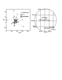
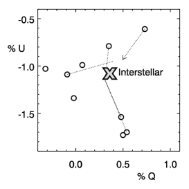
Figure 2.: Left: Polarization vector diagram of P Cyg. The magnitude of the vectors between the continuum measurements (open circles) and the zero-point polarization of P Cyg (marked ‘interstellar’) represent the strength of the intrinsic polarization; while the angle of the vector with the $Q$ axis represents the polarization’s position angle (PA). The polarization is variable in strength and PA on timescales of days. Taken from Nordsieck et al. (2001).
Right: Same as the figure on the left but for AG Car. The zero-point polarization (marked ‘interstellar’) has been determined from the H$\alpha$ depolarizations (dotted lines). Adapted from Davies et al. (2005).

In addition, we find that intrinsic polarization is more likely to be found in those objects with strong line-emission, and those that have been variable by $\mathrel{\hbox{\hbox to0.0pt{\hbox{\lower 4.0pt\hbox{$\sim$}}\hss}\hbox{$>$}}}$1 mag in the last $\sim$10 years (see Davies et al. 2005). This may be linked to the fact that the region occupied in the HR-diagram by the LBVs is close to certain instabilities, namely the bi-stability jumps and the Humphreys-Davidson limit. Strong variability in this regime means that they can often appear to stray into these zones, possibly resulting in erratic mass-loss behaviour, leading to strong line-emission and wind-inhomogeneity.

2.1. Temporal Variability

For four of our stars (AG Car, HR Car, P Cyg and R127) there exists multi-epoch data in the literature and archives (Schulte-Ladbeck et al. 1994, 1993; Leitherer et al. 1994; Clampin et al. 1995; Taylor et al. 1991; Nordsieck et al. 2001). For all four stars, the intrinsic polarization they exhibit is variable in both strength and PA (see Fig. 2). This is inconsistent with a steady axi-symmetric wind, as observed in Be stars, where we would expect the PA to remain constant. To explain the variable polarization, we considered four possible scenarios, which are summarized below (see Fig. 3). For a full discussion on each explanation and their merits, see Davies et al. (2005).

• An axi-symmetric wind with a variable optical depth, causing the polarized emission to originate from different latitudes as a function of time. In this scenario, polarization at any epoch would be aligned with one of two perpendicular directions (see Fig. 3a). As this is not observed, this rules out this scenario as the sole cause of the variability.

• A ‘flip-flopping’ wind, where the wind’s enhancement-plane switches between equatorial and bi-polar. This would again produce polarization in two perpendicular planes and can be ruled out.

• Binarity, similar to the mechanism producing the polarization observed in WR-O binary systems, see e.g. St.-Louis et al. (1987). This is unlikely due to the physical properties required of the companion; it would need to have comparable luminosity and/or mass-loss rate to the LBV. It is unlikely such an object would have not already been detected through doppler-wobble, composite spectrum, or X-rays from the wind-wind collision zone.

• A ‘clumpy’ wind, where the polarization is caused by light scattering off localised density-enhancements low in the wind. As the clumps move away from the star in the wind and new clumps are constantly being formed, the distribution of clumps and hence the net polarization will appear very different from epoch to epoch. This would produce the stochastic polarization variations we observe in LBVs (cf. Fig. 2), and is the most likely explanation.

A clumpy inner wind is consistent with the clumpy nature of these stars’ inner nebulae (e.g.  Nota et al. 1995; Chesneau et al. 2000) and the spectroscopic variability of their discrete absorption components (e.g.  Stahl et al. 2001). It is worth noting that wind-clumping is also the favoured explanation of similar polarimetric behaviour seen in WRs by e.g. Robert et al. (1989), who also find that the amplitude of the variability decreases with increasing terminal wind velocity. This is consistent with the LBVs, which have much slower winds ($\sim$200 km s^-1, compared with $\sim$1500 km s^-1), with greater polarimetric amplitude ($\sim$1% compared with $\mathrel{\hbox{\hbox to0.0pt{\hbox{\lower 4.0pt\hbox{$\sim$}}\hss}\hbox{$<$}}}$0.2%).

As an aside, the first few polarimetric observations of AG Car by Schulte-Ladbeck et al. (1994) suggested some form of axi-symmetry, leading the authors to suggest one of the first two explanations. However, these scenarios are not supported by subsequent observations (Leitherer et al. 1994; Davies et al. 2005). This highlights the pit-falls in drawing conclusions from single-epoch polarimetry data.

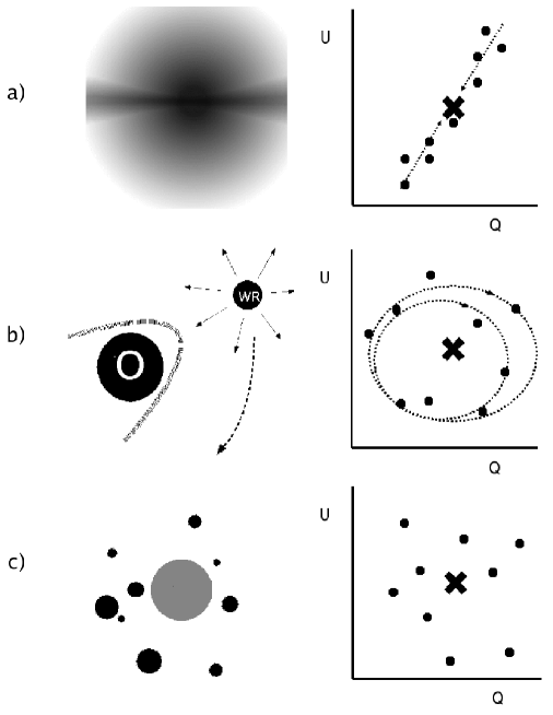
Figure 3.: Cartoons of three different scenarios capable of producing variable polarization (left), and the corresponding $Q-U$ behaviour we would expect (right). Symbols are the same as in Fig. 2.
(a): an axi-symmetric wind. When the PA of polarization is perpendicular to the disk, we measure polarization along one vector in $Q-U$ space. If the PA were to rotate by 90^∘ due to e.g. an opacity increase at the equator or a flip from equatorial to bi-polar wind, we would measure polarization along a vector on the opposite quadrant of $Q-U$ space.
(b): binarity, e.g. a WR-O system. The O star’s light is polarized due to scattering off the wind-wind collision zone. As the density enhancement region rotates with the binary system, the polarization describes a double-loop in $Q-U$ space.
(c): wind-clumping. Each clump in the wind scatters the starlight. If the clump distribution is not spherically symmetric, a net polarization results. As the clump distribution changes with time, so does the polarization.

3. Simulations of clumpy winds

In order to begin to get a handle on typical clump parameters, we have constructed an analytical model which simulates the polarimetric variability due to wind clumping. Clumps are given a typical size, optical depth, and ejection timescale. Once ejected radially from a random position on the surface of the star, the polarization of one clump is tracked as it accelarates with a $\beta=1$ velocity law. The polarization due to all the clumps in the wind is calculated as a function of time, as new clumps are ejected and move through the wind. A typical run is shown in Fig. 4. Full analysis of the models is pending (Davies et al. 2005 in prep), but initial results are summarized below.

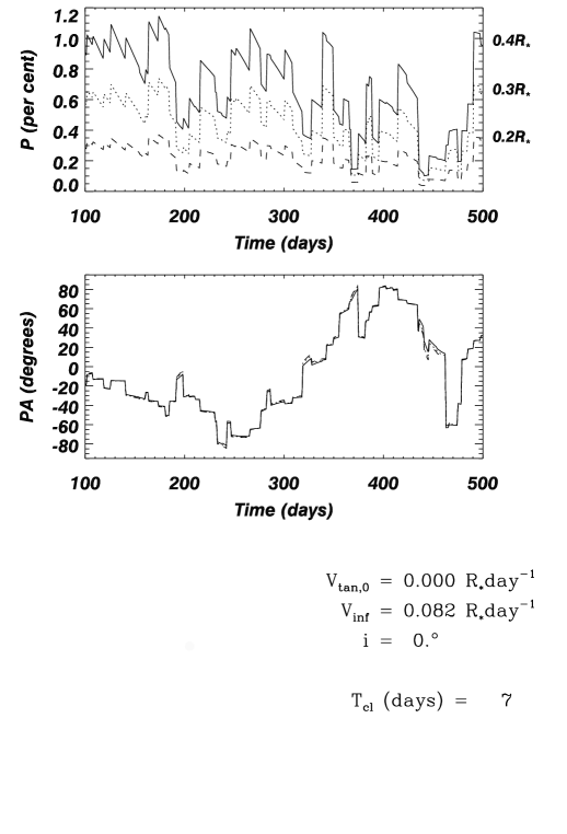
Figure 4.: Simulations of the time-dependent polarization produced by a random distribution of clumps in a spherical wind. The simulations use typical LBV parameters of $M=30$M_⊙, $R=300$R_⊙, and $v_{\infty}=$200 km s^-1; and the clumps have $\tau_{e}=1$ and ejection timescale of 7 days. Runs using three different clump sizes of $0.4$R_⋆, $0.3$R_⋆, and $0.2$R_⋆ are shown. From Davies (2005, in prep).

It can be seen that, in order to produce the observed levels of polarization and polarimetric variability, the clumps must be large ($\mathrel{\hbox{\hbox to0.0pt{\hbox{\lower 4.0pt\hbox{$\sim$}}\hss}\hbox{$>$}}}$ 0.2$R$_⋆) and ejected every few days. Increasing the density of the clumps (and hence the number of scatterers) does not allow the clump size to be reduced, as Monte-Carlo studies have shown that the polarization per clump plateaus at the $\tau_{e}\mathrel{\hbox{\hbox to0.0pt{\hbox{\lower 4.0pt\hbox{$\sim$}}\hss}\hbox{$>$}}}1$ level (Rodrigues & Magalhães 2000). Also, the polarization per clump falls off dramatically with distance. This means that (a) the clumps must be produced at or below the photosphere, not condense out of the wind at larger distances due to radiative instabilities (e.g.  Runacres & Owocki 2002); and (b) there must be a constant supply of clumps.

For a given mass-loss rate and density contrast between clump and ambient wind ($\sim$ 20, Nordsieck et al. 2001), the polarization as a function of clump size and ejection timescale can be simulated. Through polarimetric monitoring of the LBVs we will constrain the clump ejection timescale through the signature of jumps in polarization that ejection events cause (Fig. 4). From this, we can ultimately determine the volume filling-factor of the clumps, the parameter to which wind models are so sensitive (Bouret et al. 2005).

4. Summary

In the first comprehensive spectropolarimetric study of LBVs, we find that at least 50% show evidence of intrinsic polarization – over double the detection rate of WRs and O supergiants. Moreover, the polarization is stochastically variable, suggesting that the polarization is not due to axi-symmetric wind structure but instead caused by significant wind-clumping. Preliminary modelling of this shows that the clumps must be very large, and produced at/below the photosphere – clumps condensing out of the wind at large distances cannot produce the observed variability. Polarimetric monitoring will allow us to constrain further typical clump parameters, and ultimately determine the wind clump filling-factor, enabling more accurate mass-loss rate estimates.

References

- Bouret et al. (2005) Bouret, J.-C., Lanz, T., & Hillier, D. J. 2005, A&A, 438, 301
- Cassinelli et al. (1987) Cassinelli, J. P., Nordsieck, K. H., & Murison, M. A. 1987, ApJ, 317, 290
- Chesneau et al. (2000) Chesneau, O., Roche, M., Boccaletti, A., et al. 2000, A&AS, 144, 523
- Clampin et al. (1995) Clampin, M., Schulte-Ladbeck, R. E., Nota, A., et al. 1995, AJ, 110, 251
- Davies et al. (2005) Davies, B., Oudmaijer, R. D., & Vink, J. S. 2005, A&A, 439, 1107
- Harries et al. (1998) Harries, T. J., Hillier, D. J., & Howarth, I. D. 1998, MNRAS, 296, 1072
- Harries et al. (2002) Harries, T. J., Howarth, I. D., & Evans, C. J. 2002, MNRAS, 337, 341
- Humphreys & Davidson (1994) Humphreys, R. M. & Davidson, K. 1994, PASP, 106, 1025
- Leitherer et al. (1994) Leitherer, C., Allen, R., Altner, B., et al. 1994, ApJ, 428, 292
- Morris et al. (1999) Morris, P. W., Waters, L. B. F. M., Barlow, M. J., et al. 1999, Nat, 402, 502
- Nordsieck et al. (2001) Nordsieck, K. H., Wisniewski, J., Babler, B. L., et al. 2001, in P Cygni 2000: 400 Years of Progress, ed. M. de Groot & C. Sterken (ASP Conference Series v.233)
- Nota et al. (1995) Nota, A., Livio, M., Clampin, M., & Schulte-Ladbeck, R. 1995, ApJ, 448, 788
- Robert et al. (1989) Robert, C., Moffat, A. F. J., Bastien, P., Drissen, L., & St.-Louis, N. 1989, ApJ, 347, 1034
- Rodrigues & Magalhães (2000) Rodrigues, C. V. & Magalhães, A. M. 2000, ApJ, 540, 412
- Runacres & Owocki (2002) Runacres, M. C. & Owocki, S. P. 2002, A&A, 381, 1015
- Schulte-Ladbeck et al. (1994) Schulte-Ladbeck, R. E., Clayton, G. C., Hillier, D. J., Harries, T. J., & Howarth, I. D. 1994, ApJ, 429, 846
- Schulte-Ladbeck et al. (1993) Schulte-Ladbeck, R. E., Leitherer, C., Clayton, G. C., et al. 1993, ApJ, 407, 723
- St.-Louis et al. (1987) St.-Louis, N., Drissen, L., Moffat, A. F. J., Bastien, P., & Tapia, S. 1987, ApJ, 322, 870
- Stahl et al. (2001) Stahl, O., Jankovics, I., Kovács, J., et al. 2001, A&A, 375, 54
- Taylor et al. (1991) Taylor, M., Nordsieck, K. H., Schulte-Ladbeck, R. E., & Bjorkman, K. S. 1991, AJ, 102, 1197