MAGPIS: A Multi-Array Galactic Plane Imaging Survey

Abstract

We present the Multi-Array Galactic Plane Imaging Survey (MAGPIS), which maps portions of the first Galactic quadrant with an angular resolution, sensitivity and dynamic range that surpasses existing radio images of the Milky Way by more than an order of magnitude. The source detection threshold at 20 cm is in the range 1-2 mJy over the 85% of the survey region ($5\arcdeg<l<32\arcdeg,|b|<0\fdg 8$) not covered by bright extended emission. We catalog over 3000 discrete sources (diameters mostly $<30\arcsec$) and present an atlas of $\sim 400$ diffuse emission regions. New and archival data at 90 cm for the whole survey area are also presented. Comparison of our catalogs and images with the MSX mid-infrared data allow us to provide preliminary discrimination between thermal and non-thermal sources. We identify 49 high-probability supernova remnant candidates, increasing by a factor of seven the number of known remnants with diameters smaller than $5\arcmin$ in the survey region; several are pulsar wind nebula candidates and/or very small diameter remnants ($D<45\arcsec$). We report the tentative identification of several hundred H II regions based on a comparison with the mid-IR data; they range in size from unresolved ultra-compact sources to large complexes of diffuse emission on scales of half a degree. In several of the latter regions, cospatial nonthermal emission illustrates the interplay between stellar death and birth. We comment briefly on plans for followup observations and our extension of the survey; when complemented by data from ongoing X-ray and mid-IR observations, we expect MAGPIS to provide the most complete census yet obtained of the birth and death of massive stars in the Milky Way.

1. Introduction

The Milky Way is a galaxy of stars radiating most of their energy at optical wavelengths. But from stellar birth to stellar death, from the vast reaches of interstellar space to the tiniest of stellar corpses, radio and X-ray observations provide crucial diagnostics in our quest to understand the structure and evolution of our Galaxy and its denizens. These two spectral regimes are particularly crucial for studying massive stars: throughout their lives, stellar Lyman continuum photons produce H II regions with their associated free-free radio emission, while stellar wind shocks produce X-rays; in death, the remnants of supernovae are the brightest radio and X-ray sources in the Galaxy. Furthermore, the Galaxy is largely transparent in the radio and hard X-ray bands, giving us an unobstructed view through the plane, even at $b=0\arcdeg$. We are in the process of conducting a large-scale survey of the Galactic plane at X-ray wavelengths with XMM, the first results of which have been reported elsewhere (Hands et al. 2004). Here we describe a complementary effort to provide a new, high-resolution, high-sensitivity view of centimetric radio emission in the Milky Way.

While significant progress has been made recently in surveying the extragalactic radio sky (e.g., NVSS, SUMSS, and FIRST), the Galactic plane still remains inadequately explored. Even though the NVSS (Condon et al. 1998) covered the plane, it did so in snapshot mode with $uv$ coverage insufficient to achieve high dynamic range (typical values achieved are $\sim$30:1). The Canadian Galactic Plane Survey project (English et al. 1998) is covering a large region of the plane in the second quadrant with better dynamic range, but with a resolution of only $65\arcsec$ and limited sensitivity in the continuum. The third and fourth Galactic quadrants are being surveyed using Parkes and the Australia Compact Telescope Array in the Southern Galactic Plane Survey (McClure-Griffiths at al. 2001), although the angular resolution is only $\sim 2\arcmin$ and the $5\sigma$ detection threshold is $\sim 35$ mJy in the continuum.

Fifteen years ago, we used observations originally taken by Dicke et al. (unpublished) in the B-configuration of the Very Large Array (supplemented by additional 20 cm and 6 cm time awarded to us) to produce a catalog of over 4000 compact sources within a degree of the plane in the longitude range $-20\arcdeg<l<120\arcdeg$ (Becker et al. 1990; Zoonematkermani et al. 1990; White, Becker, and Helfand 1991; Helfand et al. 1992). Although the original analysis provided maps that were complete only to $\sim 20$ mJy at 20 cm, this remains the highest resolution and most sensitive census of compact sources over a large segment of the Galaxy. Comparison with the IRAS survey led us to identify more than 450 ultracompact H II regions, over 100 new planetary nebulae (which fill in the gap near $b=0$ caused by extinction in optical searches – Kistiakowsky and Helfand 1995), and, along with 90 cm maps we obtained covering a small portion of the longitude range, more than a dozen new supernova remnant candidates.

Motivated by the torrent of new, high-resolution mid-infrared data from the GLIMPSE Legacy survey with Spitzer (Benjamin et al. 2003) and taking advantage of modern data analysis algorithms developed for our FIRST survey (Becker, White & Helfand 1995; White et al. 1997), we have recently completed a reanalysis of all of the existing snapshot data (over 3000 individual pointings including some new data designed to fill holes and improve quality in poorly covered regions). This work yielded 6 and 20 cm catalogs with over 6000 entries and flux density thresholds nearly a factor of two below those of the original analysis (White, Becker & Helfand 2005). Nonetheless, the single-configuration, snapshot nature of these observations renders the data problematic for all but the most compact radio sources in the plane.

A high-sensitivity, high-resolution, high-dynamic-range map of the radio continuum emission from the Galactic plane is now possible with a relatively modest investment of telescope time owing to advances in the VLA receivers over the last decade, the implementation of the highly efficient ”survey mode” slewing algorithm, and improvements to the AIPS software package. We have begun to make this possibility a reality by producing a $5\arcsec$-resolution image of 27 degrees of Galactic longitude in the first quadrant. Our plan over the coming several years is to extend this survey over the entire Spitzer GLIMPSE longitude range in the north, covering $5\arcdeg<l<65\arcdeg$. This Multi-Array Galactic Plane Imaging Survey or MAGPIS (a moniker appropriate for the authors whose careers have been based on collecting random shiny objects gathered from overflights of much of the celestial sphere in several regions of the electromagnetic spectrum) is designed to provide a definitive archive of the Galactic sky at 20 cm.

In Section 2 we describe the survey parameters and the data acquired to date; in addition, we discuss complementary datasets we have used in our analysis and introduce the MAGPIS website, which offers comprehensive access to all of our data products. Section 3 outlines our analysis strategy, presents the imaging results, and provides a statistcal characterization of the survey sensitivity threshold and dynamic range. We then discuss our detection algorithms for both discrete and diffuse sources, and present the source catalogs as well as an atlas for all extended emission regions (§4). Section 5 includes a discussion of a preliminary comparison between MAGPIS and the MSX mid-IR data, and previews the prospects for a more complete census of H II regions in the first quadrant. This is followed by a discussion (§6) of the nonthermal emission regions detected in our survey, including the discovery of several dozen new supernova remnant candidates. We summarize our results in Section 7.

2. The MAGPIS Survey: Design and Data Aquisition

As noted above, radio emission is a prominent signature of massive stars; H II regions, pulsars, supernova remnants, and black hole binaries are all the products of O and early B stars that have a small scale height. This fact, coupled with constraints on the total observing time available, has led us to restrict our Galactic latitude coverage to $|b|<0\fdg 8$. This is greater than the OB star scale height (Reed 2000) for all distances beyond 3 kpc and covers a region up to $z=\pm 230$ pc at the solar circle on the far side of the Galaxy (we adopt $R_{\odot}=8.5$ kpc throughout).

2.1. The 20 cm data

Our first tranche of Galactic longitude, $32\arcdeg>l>19\arcdeg$, was chosen to complement our first X-ray data set and to explore the tangent to the Scutum spiral arm. The second segment we have completed covers the region $19\arcdeg>l>5\arcdeg$; we stopped at $5\arcdeg$ mainly because the central regions have been reasonably well-mapped previously. We intend to continue the survey as time becomes available, first to the GLIMPSE upper longitude limit of $l=65\arcdeg$ and later to both higher and lower longitudes.

Data are collected in the B-, C-, and D-configurations of the VLA operating in pseudo-continuum mode at 20 cm; two 25-MHz bandwidths centered at 1365 MHz and 1435 MHz are broken into seven 3 MHz channels to minimize bandwidth smearing as well as to reduce significantly our sensitivity to interference. The loss of a factor of two in bandwidth over the standard continuum mode is not important, since virtually all maps are dynamic-range, rather than sensitivity, limited.

Figure 1.— The hexagonal grid of 252 VLA pointing centers used for the MAGPIS 20 cm survey.

Figure 2.— The variation in the rms noise as a function of position after the overlapping images have been co-added. The rms is normalized to unity at field center for a single pointing. The top panel shows a cut in latitude at the edge of the survey ($l=32\arcdeg$), and the bottom panel shows the rms along a line passing near the field centers at $b=0\fdg 6$. The rms noise is uniform, with a peak-to-peak variation of only $\sim\pm 10$% except at the edges of the surveyed area.

The pointing pattern is displayed in Figure 1. The close-packed hexagonal array provides uniform coverage with a peak-to-minimum variation in sensitivity of $<20\%$ (after co-adding of adjacent images — see Fig. 2). We observe each location four times in each of the three configurations spaced roughly equally in hour angle over a range $\pm 4$ hrs to maximize $uv$ coverage; the result is an average of $\sim 12$ minutes per field per configuration, providing a theoretical noise level ($\sim 0.08$ mJy) far below the dynamic range limit of the maps. In the second round of observations we have saved observing time by using the full 12 minutes per field in the B configuration, but reducing the integration time by a factor of two in the two lower-resolution configurations (while maintaining the observational cadence at multiple hour angles). This reduces our sensitivity by $\sim 20\%$ in the least-populated map regions, although, again, most of the images are dynamic-range limited and the effect on the final source catalog is minimal.

A total of 165 hours of time has been accumulated to date in the MAGPIS project. Table 1 lists the observing epochs and configurations used to construct the 252 individual images, which cover an area of over 42 deg².

Table 1Observing Log

	VLA Configuration
Description	B	C	D	BnC
Phase 1, 20 cm	Mar–Apr 2001	Aug–Sept 2001	Aug–Sept 2000	May 2001
	31 hrs	28 hrs	28 hrs	1.5 hrs
Phase 2, 20 cm	Jan 2004	Feb–Mar 2004	Apr 2003
	36 hrs	19 hrs	18 hrs
Phase 1, 90 cm		Sept 2001
		3.5 hrs

2.2. The 90 cm data

Even with high-quality images, a single frequency is insufficient to identify source classes unambiguously and to disentangle thermal and nonthermal emission in crowded regions. As part of our initial observation program for MAGPIS, we obtained 3.5 hours of 90 cm pseudo-continuum observations in the C configuration of the VLA during September of 2001. Eight pointings were used to cover the region $20\arcdeg<l<33\arcdeg,|b|<2\arcdeg$. The data were reduced using a $15\arcsec$ pixel size and have a resolution of $\sim 70\arcsec$. In addition, we retrieved from the VLA archive 90 cm data originally taken by Brogan et al. (2005) that cover the remainder of our current survey area ($3\fdg 6<l<20\arcdeg,|b|<2\arcdeg$). These data were reduced using a $6\arcsec$ pixel size and have a resolution of $\sim 25\arcsec$.

2.3. The mid-IR data

We have retrieved the mid-IR images and catalogs of the Midcourse Space Experiment (MSX – Price et al. 2001) from the IPAC database for the regions our survey covers to date. For ease of comparison, we have regridded the E-band ($20\,\mu$m) data onto the same $l,b$ grid used to present the primary MAGPIS images. We have also constructed ratio maps for the 20 cm and $20\,\mu$m data for use in separating thermal and nonthermal emission. An example of such an image is displayed in Figure 3. High values of the radio-to-IR ratio generally indicate nonthermal radio emission such as is produced by supernova remnants, while low values tend to highlight dusty H II regions, although pulsar wind nebulae, dusty old supernova remnant shells, and dust-free H II regions can in principle exhibit intermediate ratios. We defer a quantitative discussion of the comparison of the radio and mid-IR emission to a future paper.

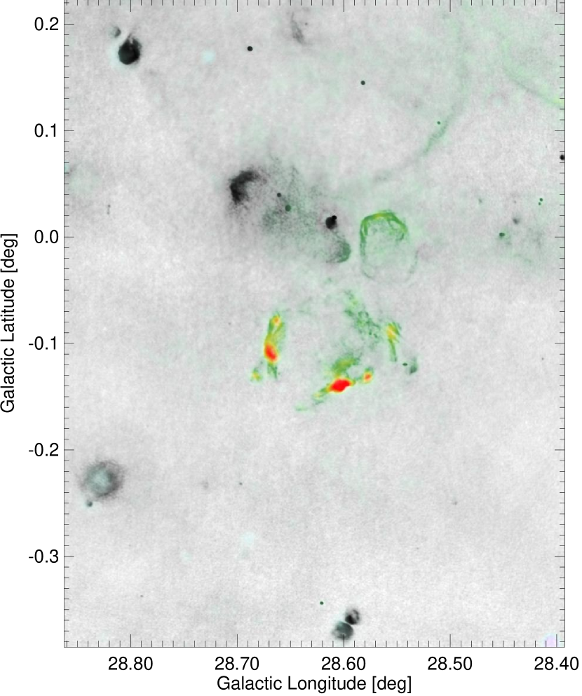
Figure 3.— Combined radio-IR image demonstrating the separation of thermal and non-thermal emission. The radio image is used to set the intensity of the displayed image, while the radio-IR flux ratio is used to set the color hue and saturation. Objects with strong IR emission (typical of thermal radio sources) appear in black and white, while objects that have absent or weak IR emission (typical of nonthermal radio sources) appear in colors ranging from green to red depending on the upper limit on the radio-to-IR ratio. Both the known SNR G28.6-0.1 and a previously undiscovered remnant at G28.56-0.01 are apparent, as are a half-dozen thermal sources with varying morphologies.

2.4. The MAGPIS website

Consistent with our past practice, the raw VLA data on which MAGPIS is based have been available in the VLA archive from the day they were taken. To facilitate use of these data by the broadest possible community, we have constructed the MAGPIS website (http://third.ucllnl.org/gps), which presents our data products in easily accessible forms. In addition to the full-resolution 20 cm images, the site provides the complementary 90 cm images, the regridded MSX $20\,\mu$m images, and an image atlas of diffuse emission regions (see below). The single-configuration 6 and 20 cm images from our earlier snapshot surveys (White, Becker & Helfand 2005) are also available. Images can be displayed with user-specified coordinates, box sizes, and intensity scales or can be downloaded as FITS files. The full discrete-source and diffuse catalogs are available for retrieval or through a search query function, as are our catalogs and publications from our earlier snapshot survey work. We expect to add our XMM X-ray survey data and the Spitzer GLIMPSE survey images and catalogs as they become available.

3. The MAGPIS Images

In contrast to the extragalactic radio sky, which is rather sparsely populated by mostly compact sources, radio emission in the Galactic plane is dominated by bright, diffuse H II regions and supernova remnants. Thus, the single-snapshot observations and two-dimensional mapping approximations that worked well in the FIRST and NVSS surveys are inadequate for producing high-dynamic-range images for MAGPIS. In this case, the VLA data must be treated as a three-dimensional data set. In practice, 3-d distortions scale with offset from the image center; thus, one way to minimize 3-d effects is to tile the VLA’s $30\arcmin$ primary beam with many small images. We have used a grid of 21 by 21 images, each of which is 128 by 128 pixels in size. Our initial data were reduced on a Sun Ultra 60, with each image requiring $\sim 12$ hours to CLEAN. We subsequently migrated the analysis to a dual-processor Pentium 4 computer that is approximately seven times faster. Since the images are greatly improved by self-calibration, each field has to be reprocessed several times.

Even with data from the D configuration, the resulting maps suffer missing flux from large-scale structure ($\gg 1\arcmin$) to which the VLA is insensitive. To correct for this deficiency, we combined the VLA images with images from a 1400 MHz survey made with the Effelsberg 100-m telescope ($\sim 7\arcmin$ angular resolution). The AIPS task IMERG makes FFTs of both the VLA and Effelsberg images, combines the derived FFT amplitudes, and then converts back to the image plane to produce the final individual images. We use a $6\farcs 2\times 5\farcs 4$ restoring beam on maps with a pixel size of $2\farcs$. The individual maps are ultimately summed and rebinned to produce mosaic images in Galactic coordinates. The dynamic range varies somewhat with location but, measured as a ratio of the peak flux in the brightest source to the full image rms, is typically in excess of 1000:1 in a 1 deg² image. Over most of the images, 1 mJy point sources are easily detected.

4. The MAGPIS Catalogs

The large, diffuse emission features and variable background, coupled with source size scales ranging from arcseconds to degrees, render impractical the type of automated source detection algorithms applied to extragalactic radio surveys. Thus, we have employed the human eye-brain detection system to search the 16.7 million MAGPIS beam areas for radio sources. We divided the problem into two parts: the detection and cataloging of discrete objects less than a few beam areas in size and unconfused by extensive diffuse emission, and regions of sky in which significant diffuse emission is present.

4.1. Discrete source detection

A square field was defined around each candidate discrete source. In cases where it was impossible to isolate a single emission peak (e.g., for overlapping or closely clustered sources), multiple sources were included in one field and the field was flagged as ”multiple”. The default field size was $34\arcsec\times 34\arcsec$, but this size was adjusted for larger sources (increased), for high density areas (decreased), or for other reasons (increased or decreased on a case by case basis) such as nearby bad pixels, proximity to the edge of the maps, etc. For the entire survey area this process yielded 2628 single-source fields, and 467 multiple-source fields.

The AIPS task HAPPY (see White et al. 1997) was then run on each of the fields. In HAPPY, a local rms level was calculated for each field using an area of three times the input field area; a minimum detection level of five times the local rms was set for each field.

Using the HAPPY output, we rejected any source with a fitted peak flux, $F_{p}<1.0$ mJy or $\leq 5.0$ times the local rms, whichever is higher. We also rejected any source with a fitted minor axis less than $3\farcs 5$ (the beam minor axis is $5\farcs 2$, and experience from the use of HAPPY in the FIRST survey shows that the vast majority of such “skinny” sources are spurious sidelobes); this only eliminated one source that passed the $F_{p}$ and rms criteria. This process yielded a catalog of 3229 sources.

Although restricting HAPPY to predetermined fields around candidate sources should reduce the number of spurious detections, this method is still susceptible to poor fits resulting from complex, extended emission as well as areas of patterned noise near bright sources. To assess these potential causes of contamination, we flagged for further examination HAPPY solutions

1. when HAPPY fit more than one source in a single-source input field (67 fields, 144 sources);

2. when HAPPY fit more than two sources in a multiple-source input field (69 fields, 219 sources); or

3. when any fit not meeting (1) or (2) had a major axis $>15\arcsec$, a major to minor axis ratio greater than 2.0, or $F_{int}/F_{p}>5.0$ (136 fields, 143 sources).

In total, 506 fields were flagged and examined. Of these 338 were determined to be good fits, 88 to be “acceptable” fits, 56 to be artifacts or noise, and 24 to be extended rather than discrete sources; the latter were moved to the extended source atlas (see below) and the artifacts were deleted.

The 88 “acceptable” fits are all (in our best judgement) real radio sources, but they are distinguished from good fits in that, upon inspection, it is clear that the two-dimensional Gaussian employed by HAPPY is a poor representation of the source surface brightness distribution. We report their HAPPY-derived parameters in Table 2 for consistency, but flag them accordingly.

The final catalog, presented in Table 2, includes 3149 discrete sources. A Galactic longitude $\pm$ latitude-based name (col. 1) is followed by the peak and integrated flux densities from the Gaussian fit (cols. 2 and 3), with the $S_{i}$ value flagged for the “acceptable” fits described above, and the estimated rms noise level (col. 4). The major and minor axes (full-width at half-maximum) and position angle for the elliptical Gaussian complete the morphological description of these compact sources. The last two columns give the infrared 8 $\mu$m and 21 $\mu$m flux densities for sources with MSX matches (described further below in §5.1).

Owing to the variable background and numerous regions of bright diffuse emission, the threshold for discrete source detection varies significantly over the survey region. We can obtain a mean value for the threshold by comparing the source surface density with that of the FIRST survey. That survey covers 9033 deg² of the extragalactic sky and includes 781,450 sources not flagged as sidelobes, for a mean surface density of 86.54 deg^-2 at a flux density threshold of 1.0 mJy. The mean source surface density of discrete sources in MAGPIS is 74.8 deg^-2 considering the entire survey area of 42.1 deg² and 73.0 deg^-2 in the 35.6 deg² lying outside regions of diffuse emission; the former value is higher owing to source clustering. Matching this surface density while allowing for several hundred true Galactic sources outside regions of diffuse emission (see §5.1), we find an effective discrete source threshold of $\sim 1.5$ mJy that yields 58.6 extragalactic sources deg^-2 in FIRST. Thus, our survey is significantly incomplete between the minimum reported flux density of 1 mJy and $\sim 2$ mJy, but, over the 85% of the area outside regions of diffuse emission, it is largely complete above this range. Note that a large majority of the discrete radio sources detected even within $1\arcdeg$ of the Galactic plane are extragalactic objects; this is evident from the lack of a strong Galactic latitude dependence of our source counts seen in Figure 4. Observations at other wavelengths are required to identify the Galactic components of the discrete source population.

Figure 4.— Galactic latitude distribution for the discrete source catalog. Even in the Galactic plane the 20 cm radio sky is dominated by extragalactic sources, so no strong latitude dependence is seen. The counts fall off in the $|b|>45$ arcmin bins due to the drop in sensitivity at the edge of the survey.

4.2. The diffuse source atlas

The elliptical Gaussians used in fitting the discrete sources are a poor approximation to the surface brightness distributions for nearly all of the more extended radio sources detected in our survey. Furthermore, for sources extended by more than $\sim 60\arcsec$, our VLA $uv$ coverage is inadequate to derive accurate flux densities, and the addition of the single dish data, while an asset in making images, has unquantifiable effects on derived flux densities. Thus, we again turn to the eye-brain system for identifying diffuse sources and source complexes, and do not attempt to derive accurate flux density measurements for these sources.

The entire survey region was examined by eye, and regions of extended emission were identified and enclosed in square boxes ranging in size from 1 arcmin² to $48\arcmin\times 48\arcmin$. In some instances regions are defined by a single coherent source, while in others a complex of diffuse emission regions is included. A total of 398 such regions covering 7.6 deg² were so identified. For each region, the peak flux density, minimum flux density (a proxy for the noise level in the region), total area, and net flux density were recorded; we emphasize that these flux densities are not necessarily accurate reflections of integrated source intensity and, in some regions, include the flux density of several related – or possibly unrelated – sources; they provide only a rough guide to source intensities. We have subtracted from the integrated flux density in each region the sum of the flux densities of the discrete sources from Table 2 that fall within the region; a table listing the cataloged discrete sources within each region is available at the MAGPIS website.

In order to estimate the accuracy of our diffuse flux density estimates, we have compared our flux densities for the 25 known supernova remnants in our survey region with those tabulated in Green (2004). We exclude remnants for which the tabulated value is uncertain (listed with a “?” in Green’s catalog), as well as those that do not fall completely within our survey coverage. We scale the 1.0 GHz flux densities listed in Green’s catalog to our observing frequency of 1.4 GHz using the tabulated spectral indices. We find a good correlation between the flux densities, albeit with an offset that depends on the size of the remnant (Fig. 5). We conclude that the integrated flux densities listed for the diffuse sources typically overestimate the true fluxes of very large sources by factors of two or more due to backgrounds and confusing sources and recommend caution when using them.

Figure 5.— Flux densities from our diffuse source catalog for supernova remnants from the Green (2004) catalog. The x symbols show that our catalog flux densities for these extended sources are typically higher than the Green values by factors of two or more. Subtracting a corrective offset of 0.07 Jy/arcmin² from our flux densities improves the agreement (dots).

The diffuse regions are cataloged in Table 3. A Galactic longitude$\pm$ latitude-based name is found in column 1. The box size in column 2 and an intensity scaling factor for display purposes (col. 3) precede the brightest pixel value (col. 4) and its location (cols. 5 & 6), the minimum flux density recorded in the box (col. 7), and the integrated flux density inside the box (col. 8). Column 9 provides names for known supernova remnants.

Cleaving to the maxim that quantifies the relative information content of words and pictures, we have constructed a diffuse source atlas to accompany the full survey images on the MAGPIS website. Here, Table 3 is reproduced with active links that allow the user to overlay circles representing sources from the discrete source catalog and contours of the $20\,\mu$m images from the MSX catalog (Eagen et al. 2003). Each image can also be downloaded as a FITS file.

The website also includes large area ($4\fdg 5\times 1\fdg 6$) JPEG versions of the MAGPIS images with the diffuse region boxes overplotted. It is difficult to display these high-dynamic-range images with a single constrast stretch, and indeed the discrete sources are almost invisible in these images, but they are nonetheless useful for viewing the environment of the diffuse sources.

The MAGPIS discrete source catalog and diffuse source atlas provide an improvement of more than an order of magnitude in both angular resolution and sensitivity over existing Galactic plane survey data. When combined with existing catalogs at other wavelengths along with data from X-ray and infrared surveys currently underway, MAGPIS will provide a resource for studying both thermal and nonthermal processes that mark the evolution of massive stars in the Milky Way. We have a number of followup projects underway; below we briefly comment on the impact the survey is likely to have on our knowledge of the H II region and supernova remnant populations of the Galaxy.

5. Galactic Thermal Emission Regions: MAGPIS and Mid-IR Images

The critical dependence of an H II region’s radio luminosity on the ionizing flux of its exciting star(s) allow for the contruction of a particularly pure census of massive star formation: the 20cm radio flux density falls by a factor of 300 between exciting star types O9.5 and B1 such that, at 20 kpc, O-star H II regions fall a factor of $>30$ above our survey threshold, while less-massive star-forming complexes (which produce at most B stars) fall a factor $>10$ below it. To separate the H II regions from the more numerous extragalactic source populations and the extended regions of Galactic nonthermal emission requires observations at another wavelength. Our 6 cm snapshot survey is useful for the most compact sources ($D<15\arcsec$) but resolves out flux on larger scales. Since most H II regions also contain dust that is heated by the stellar radiation, the mid-IR also can serve as a useful discrimnant.

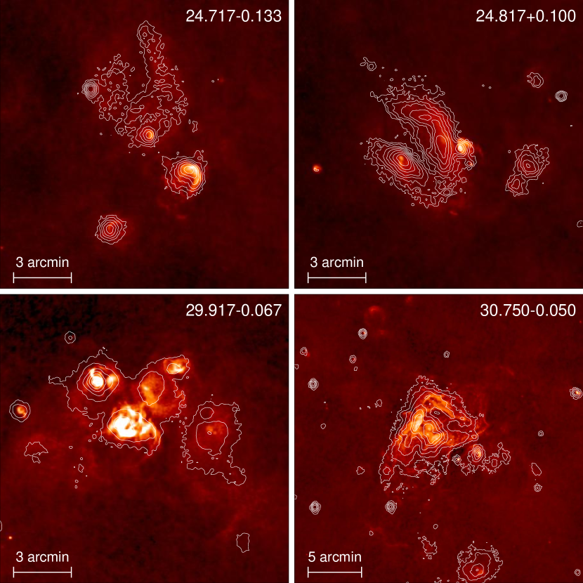
Figure 6.— Examples of H II complexes from our radio survey with the MSX $20\,\mu$m image contours overlaid, showing the excellent radio-IR correspondence for these thermal sources.

Figure 6 shows several examples of H II complexes from our radio survey with contours from the MSX $20\,\mu$m images overlaid. The degree of correspondence is remarkably good and provides a straightforward method for separating thermal and nonthermal emission in star formation regions. On the MAGPIS website we also provide large-scale radio images with boxes marking the previously published H II regions collected in the Paladini et al. (2003) meta-catalog. It is clear that the MAGPIS data (along with other radio and IR surveys) will enable the construction of a vastly improved H II region catalog.

We defer a detailed analysis of the H II region population to a future paper; here we provide some simple statistics for compact and ultracompact H II regions by matching our discrete source data to the MSX catalogs as an indication of the wealth of information such a comparison contains. The higher-resolution and greater sensitivity of the Spitzer GLIMPSE data soon to become available will fill in the 2–8$\,\mu$m band and provide crucial information in the most crowded regions.

5.1. Match to the MSX $20\,\mu$m catalog

The 20cm survey region is completely covered by the MSXPSCv2.3 ”MSX6C” (Egan et al 2003) data set. We searched for MSX6C sources using a search radius of $12\arcsec$ around each of the discrete 20 cm sources. To be accepted as a match, the MSX6C source was required to have a quality flag of 2 in at least one of the four bands (see Lumsden et al. 2002). If more than one MSX6C source fell within the search radius for a single 20 cm source, the MSX6C source closest to the 20 cm source was kept (this only occurred once). A total of 376 MSX6C sources corresponding to 418 20 cm sources were matched in this manner.

To estimate the number of false matches we repeated the matching process using fake catalogs produced by shifting the MSX6C catalog $\pm 10\arcmin$ and $\pm 20\arcmin$ in longitude. Since, for example, the vast majority (78%) of the MSX sources are stars detected only in the $8\,\mu$m band (very few of which have radio counterparts), we can greatly reduce the false match rate by assessing the false rates separately for sources detected in different band combinations. We have followed the methology descibed in Giveon et al. (2004; see also White et al. 1991), to arrive at a false-match reliability criterion for each of the band combinations in which a 20 cm-MSX6C match existed. Using a reliability of $R>90\%$ we find 245 MSX6C sources (of which $\sim 8$ should be false) matched to 278 20 cm sources. Of these, 217 are single 20 cm-MSX6C matches, 23 are cases in which one MSX6C source matches two 20 cm sources, and 5 represent one MSX6C source matching three 20 cm sources.

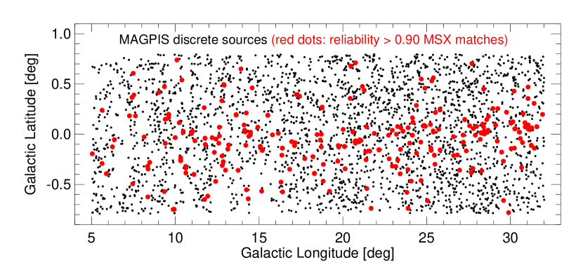
Figure 7.— Sky distribution of MAGPIS 20 cm radio sources from the discrete source catalog. Red dots show sources with confident (reliability $>0.90$) infrared counterparts in the MSX catalog. The radio-MSX matches are clearly concentrated toward the plane.

Figure 8.— Galactic latitude distribution for the 245 MSX sources having reliable radio matches. These sources are highly concentrated toward the plane of the Galactic disk.

The distribution of the matched and unmatched sources on the sky is displayed in Figure 7. While sources with infrared matches are found throughout the latitude coverage, it is clear that they concentrate toward the plane. The latitude distribution is displayed in Figure 8. The distribution peaks at $b=0\arcdeg$ with a surface density of 22 sources deg^-2 (when regions obscured by bright diffuse sources are excluded), and has a full width half maximumn of less than $15\arcmin$. Examination of the atlas of extended emission shows that there are more thermal sources inside the 6.5 deg² subsumed by the atlas images than outside, and most of these sources are not included in the discrete source catalog. We estimate that there are a total of more than 600 distinct H II regions in our 42 deg² survey area, although we defer to a future publication the development of a detailed catalog and its analysis.

6. Galactic Nonthermal Emission in MAGPIS

Supernova remnants (SNRs) are among the brightest radio sources – and the brightest X-ray sources – in the Galaxy. They are a dominant source of mechanical energy input to the ISM, drive the Galaxy’s chemical evolution, and mark the birthsites of neutron stars and black holes. Yet our knowledge of the Galactic population is woefully incomplete, owing to the low angular resolution of previous radio and hard X-ray surveys of the plane, and the soft spectral response of previous X-ray imaging observations. A total of 231 remnants appears in the latest catalog (Green 2004); Brogan et al. (2004) have recently added three new remnants in one of our fields. The current rate of discovery is a few remnants per year. However, based on 1) extragalactic SN rates ($\sim$ 1–2 per century) combined with SNR lifetimes (2.5-5$\times 10^{4}$ yr), and 2) a detailed analysis of the current SNR distribution (Helfand et al. 1989), we expect the total population to be between 500 and 1000. The youngest remnant we know is 340 years old; four to seven younger ones exist somewhere in the Galaxy.

MAGPIS can detect pulsar-driven remnants to a luminosity $10^{-4}$ that of the Crab Nebula at the edge of the Galaxy (or $\sim$ 10% that of 3C58, the least luminous young Crab-like remnant known). For shell-like SNRs, our survey will be sensitive to all young remnants. For example, we will detect remnants throughout the surveyed volume down to luminosities 0.01% that of Cas A, and can even see a clone of the underluminous historical remnant SN 1006 at 20 kpc: it would appear as a $1\arcmin$-diameter source with a flux density of $\sim 25$ mJy. Our survey could detect a remnant equivalent to SN87A from the time it was 3 years old anywhere in the survey region, and would resolve such a remnant only 15 years after the explosion.

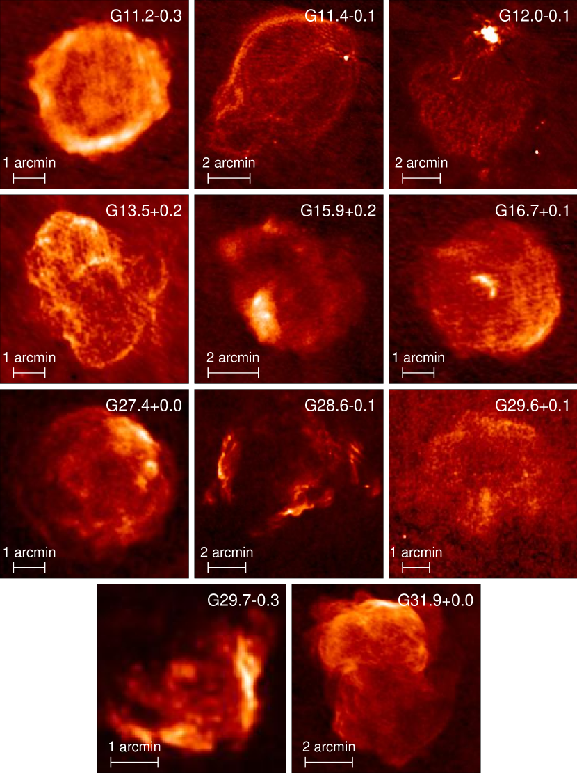
Figure 9.— MAGPIS 20 cm images of the eleven known supernova remnants in the survey area with diameters less than $10\arcmin$.

Twenty-five known remnants fall within the current survey area, and all are easily detected. The known remnants are indicated in Table 3; in many instances, the maps presented here are the best available. Images for the eleven remnants smaller than $10\arcmin$ in diameter — most of which lack high-resolution maps in the literature — are displayed in Figure 9.

As can be seen by browsing the diffuse-source atlas, there are a large number of shell-like sources detected in our survey. Without observations at other wavelengths, however, it is impossible to separate the thermal and non-thermal sources to derive a list of new SNR candidates. Fortunately, as noted above, we do have VLA data covering the entire region at 90 cm, as well as the MSX mid-IR images. A simple qualitative comparison of these three datasets (available for the reader at the MAGPIS website) allows us to identify quickly high-probablity SNR candidates.

In Table 4, we present 49 new SNR candidates in our $27\arcdeg$ slice of Galactic longitude. To derive this list, we have required:

• the object has a very high ratio of 20 cm to $20\,\mu$m flux (i.e., it is typically undetectable in the 20$\,\mu$m MSX image);

• the object has a counterpart in our 90 cm images with a similar morphology and a higher peak flux density; and

• the object has a distinctive SNR morphology. For shell-type remnants we require at least half of a complete shell, while for the two pulsar wind nebula candidates we see a centrally peaked brightness distribution.

For most of these candidates the data in columns 1, 3, 4 and 5 are repeated from Table 3. Column 2 gives the source diameter (as opposed to the display box size in column 3, which is always larger). Five of the the entries in this table are components of larger sources listed in Table 3, with three associated with the large diffuse complex at G19.60${-}$0.20 and two associated with G6.50${-}$0.48.

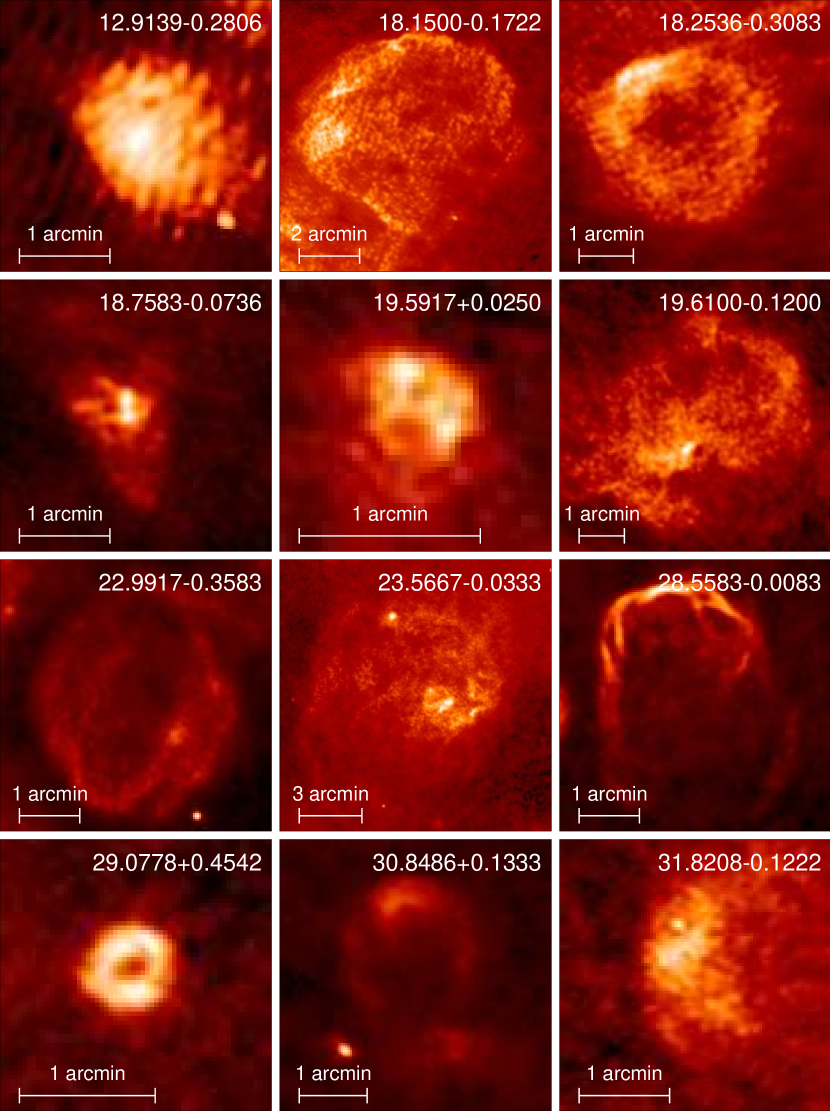
Figure 10.— MAGPIS 20 cm images of 12 new supernova remnant candidates.

Images for a dozen candidates ranging in size from $40\arcsec$ to $9\arcmin$ are displayed in Figure 10. Not unexpectedly, the diameter distribution for our remnant candidates varies markedly from that of the known remnant population. Assuming that followup spectral and polarimetric observations confirm the large majority of these sources as SNRs, we will have tripled the number of known remnants in this region of the Galaxy. However, while the number of remnants with $D\geq 10\arcmin$ will only rise from 13 to 16, the number with $10\arcmin>D\geq 5\arcmin$ will quadruple from 5 to 19, while the number with $D<5\arcmin$ will rise more than sevenfold from 5 to 37.

Particularly interesting among these new SNR candidates are those that may harbor young, high-$\dot{E}$ pulsars. In addition to the two PWN candidates, there are two shell-like remnants with central diffuse emission peaks highly reminiscent of composite SNRs. Given the core-collapse SN rate in the Galaxy, we should expect to find $\sim 10$ neutron stars younger than the Crab and 3C58 pulsars. While these new sources are significantly dimmer than even the underluminous PWN 3C58, if they are at distances of $\sim 15$ kpc, their luminosities are comparable. Also noteworthy are the three shell-type remnants with diameters less than $1\arcmin$. At 15 kpc, their diameters are $\sim 3$ pc, corresponding to an age of $\sim 130$ years for a radio expansion rate comparable to that of SN87A.

The SNR candidates listed in Table 4 far from exhaust the nonthermal emission features in our survey area; a roughly comparable number of filaments and arcs with apparently nonthermal radio spectra and no IR counterparts are seen. Furthermore, there are several regions in which thermal and nonthermal features are cospatial; these will require scaled-array observations at several frequencies to disentangle. Nontheless, it is clear that high-dynamic-range, high-sensitivity observations of the type reported here are essential for characterizing fully the Galactic SNR population.

7. Summary and Future Prospects

We have presented a centimetric image of the plane of the Milky Way in the first quadrant that represents an improvement over existing surveys by more than an order of magnitude in resolution, sensitivity, and dynamic range. The survey detection threshold is 1 to 2 mJy over most of the survey area. We identify over 3000 discrete radio sources and $\sim 400$ regions of diffuse emission, presenting catalogs and atlases that quantify the source properties. We include complementary 90 cm images over the entire survey region and provide a comparison with mid-IR data; taken together, these latter two datasets help to separate thermal from nonthermal emssion regions. We find several hundred H II regions in the survey area, many reported here for the first time. We also identify 49 high-probability supernova remnant candidates, including a seven-fold increase in the number of remnants with diameters smaller than $5\arcmin$ in the survey region. All of the survey’s results are available at the MAGPIS website.

Considerable work remains to exploit fully the survey results. A complementary hard X-ray survey over portions of this region is being conducted with XMM-Newton, and several followup obervations of interesting sources are scheduled with XMM and Chandra. Scaled-array polarimetric and photometric observations with the VLA are required to confirm the SNR candidates. As the Spitzer GLIMPSE program images become available, further progress will be possible in identifying compact and ultra-compact H II regions and in using these to provide a census of the OB star population; higher frequency observations with the VLA will be required to identify optically thick H II regions. Future observations to extend the MAGPIS coverage area will provide the basis for a comprehensive view of massive star birth and death in the Milky Way.

Table 2Catalog of Discrete Sources

Name ($l+b$)	$S_{p}$(20cm)	$S_{i}$(20cm)	RMS	Major	Minor	$\theta$	S(8$\mu$m)	S(21$\mu$m)
°	mJy/beam	mJy	mJy	″	″	°	Jy	Jy
(1)	(2)	(3)	(4)	(5)	(6)	(7)	(8)	(9)
10.74968${-}$0.41783	01.69	007.07string	0.291	15.1	09.2	54.2	$\cdots$	$\cdots$
10.78586${-}$0.14376	12.86	015.14string	0.224	06.7	05.9	36.7	$\cdots$	$\cdots$
10.80070${+}$0.15285	05.28	006.51string	0.162	06.8	06.1	18.0	$\cdots$	$\cdots$
10.81109${+}$0.75435	01.92	002.49string	0.293	08.5	05.1	83.2	$\cdots$	$\cdots$
10.82677${-}$0.01064	03.98	026.58E	0.275	17.5	12.8	16.3	$1.10$	$1.56$
10.82960${-}$0.01145	02.05	006.68E	0.275	15.6	07.0	48.5	$\cdots$	$\cdots$
10.85201${-}$0.44069	06.61	009.99string	0.222	07.3	06.9	116.2	$\cdots$	$\cdots$
10.86448${-}$0.32989	02.32	003.28string	0.365	07.3	06.5	60.3	$\cdots$	$\cdots$
10.89153${+}$0.09971	03.67	004.39string	0.278	07.2	05.6	175.7	$\cdots$	$\cdots$
10.89487${+}$0.06428	04.00	004.93string	0.388	06.8	06.0	1.3	$\cdots$	$\cdots$
10.89530${+}$0.19694	01.62	004.32string	0.180	12.6	07.1	54.2	$\cdots$	$\cdots$
10.89687${+}$0.19994	04.04	006.13string	0.180	07.6	06.7	31.6	$\cdots$	$\cdots$
10.89866${+}$0.20285	01.19	003.28string	0.180	11.3	08.2	116.6	$\cdots$	$\cdots$
10.91317${+}$0.23448	30.65	051.38string	0.207	08.2	06.9	137.6	$0.16$	$<1.34$
10.91841${-}$0.48325	01.36	002.54string	0.218	09.9	06.3	9.1	$\cdots$	$\cdots$
10.92542${+}$0.02681	69.34	083.74string	0.308	06.6	06.2	32.0	$\cdots$	$\cdots$
10.93848${+}$0.41073	02.58	002.93string	0.203	06.9	05.5	41.9	$\cdots$	$\cdots$
10.94310${-}$0.40329	05.73	022.67string	0.258	12.4	10.6	94.2	$\cdots$	$\cdots$
10.94413${+}$0.63106	04.33	005.63string	0.186	06.8	06.4	2.9	$\cdots$	$\cdots$
10.95074${+}$0.23027	01.78	002.28string	0.236	07.1	06.0	155.7	$\cdots$	$\cdots$
10.95235${-}$0.48679	01.17	002.45string	0.217	09.9	07.1	77.8	$\cdots$	$\cdots$
10.95854${+}$0.02233	37.32	047.92string	0.395	06.8	06.3	27.7	$0.35$	$12.58$
10.96456${+}$0.00641	24.92	196.93E	0.370	23.7	11.2	168.1	$1.95$	$11.42$
10.96557${+}$0.00971	46.57	207.93string	0.370	14.7	10.2	159.4	$1.95$	$11.42$
10.96678${+}$0.45096	08.77	010.53string	0.204	06.6	06.1	37.2	$\cdots$	$\cdots$
10.97994${+}$0.47065	01.66	002.76string	0.213	07.8	07.1	44.1	$\cdots$	$\cdots$
10.98345${+}$0.46966	01.26	002.33string	0.213	09.4	06.6	67.0	$\cdots$	$\cdots$
10.98584${+}$0.70115	47.01	049.54string	0.214	06.4	05.5	28.8	$\cdots$	$\cdots$
10.99897${+}$0.16847	22.35	026.37string	0.225	06.5	06.1	26.8	$\cdots$	$\cdots$
11.00796${+}$0.58933	17.50	018.61string	0.166	06.5	05.5	30.9	$\cdots$	$\cdots$
11.02311${+}$0.32766	02.35	002.94string	0.229	06.8	06.2	170.8	$\cdots$	$\cdots$
11.02444${+}$0.25564	03.39	004.10string	0.217	06.7	06.1	0.6	$\cdots$	$\cdots$
11.03023${+}$0.05336	05.64	014.01string	0.318	09.8	08.5	92.3	$\cdots$	$\cdots$
11.03291${+}$0.02761	02.95	003.71string	0.280	07.0	06.0	71.9	$0.44$	$2.52$
11.03867${-}$0.03903	06.80	007.98string	0.267	06.6	06.0	29.0	$\cdots$	$\cdots$
11.04064${+}$0.61702	01.43	001.29string	0.164	06.8	04.4	14.4	$\cdots$	$\cdots$
11.04432${+}$0.36909	03.86	004.48string	0.215	06.7	05.8	25.7	$\cdots$	$\cdots$
11.05374${+}$0.47840	03.00	002.94string	0.208	06.7	04.9	24.0	$\cdots$	$\cdots$
11.05432${+}$0.48628	74.63	079.12string	0.204	06.3	05.6	30.3	$\cdots$	$\cdots$
11.06609${+}$0.12835	01.92	002.97string	0.238	09.3	05.6	29.0	$\cdots$	$\cdots$
11.07328${+}$0.60324	01.47	001.83string	0.146	07.4	05.6	50.7	$\cdots$	$\cdots$
11.07971${+}$0.12145	01.78	003.67string	0.236	10.6	06.5	31.8	$\cdots$	$\cdots$
11.11013${-}$0.39894	87.96	253.15string	0.422	10.8	08.9	22.3	$5.05$	$68.05$
11.11020${-}$0.40122	32.79	127.79string	0.422	14.9	08.8	177.1	$5.05$	$68.05$
11.11674${-}$0.65359	01.79	003.81string	0.259	10.2	07.0	132.5	$\cdots$	$\cdots$
11.11810${-}$0.65584	01.45	003.08string	0.259	12.8	05.5	35.3	$\cdots$	$\cdots$
11.13753${-}$0.21337	04.82	006.26string	0.191	07.2	06.0	41.8	$\cdots$	$\cdots$
11.14507${-}$0.14098	01.12	002.17string	0.192	10.5	06.2	42.6	$\cdots$	$\cdots$
11.14767${+}$0.70009	01.65	002.82string	0.185	09.0	06.3	176.6	$\cdots$	$\cdots$
11.16342${+}$0.77554	01.67	005.11string	0.262	11.4	08.9	156.2	$\cdots$	$\cdots$

Note. — Table 2 is published in its entirety in the electronic edition of the Astronomical Journal and is also available on the MAGPIS website (http://third.ucllnl.org/gps). A portion is shown here for guidance regarding its form and content.

Table 3Catalog of Diffuse Emission Regions

Name ($l+b$)	Box Size	Scale	$S_{p}$	$l_{p}$	$b_{p}$	$S_{i}$	Comment
°	arcmin	mJy/beam	mJy/beam	°	°	Jy
(1)	(2)	(3)	(4)	(5)	(6)	(7)	(8)
5.1917${-}$0.2833	02.0	015.0	017.0	5.1903	${-}$0.2838	001.050
5.4444${+}$0.2056	01.0	003.0	002.3	5.4466	${+}$0.2052	000.136
5.4667${+}$0.3833	06.0	001.0	001.7	5.5155	${+}$0.3474	001.920
5.4750${-}$0.2458	06.0	007.0	114.3	5.4749	${-}$0.2432	004.040
5.5250${+}$0.0292	04.0	005.0	007.5	5.5228	${+}$0.0285	001.040
5.9000${-}$0.4333	20.0	020.0	199.5	5.8851	${-}$0.3924	056.900
5.9306${-}$0.0972	02.0	004.0	003.8	5.9301	${-}$0.0992	000.481
5.9500${+}$0.0833	25.0	010.0	175.7	5.9440	${+}$0.2013	047.900
6.0158${-}$0.3650	02.0	005.0	005.5	6.0146	${-}$0.3647	000.765
6.0806${-}$0.1167	05.0	010.0	016.1	6.0818	${-}$0.1181	006.070
6.1000${+}$0.5000	25.0	004.0	007.1	6.1624	${+}$0.4969	017.300
6.1075${-}$0.1731	01.0	005.0	006.1	6.1085	${-}$0.1720	000.289
6.1500${-}$0.6250	06.0	005.0	005.1	6.1346	${-}$0.6352	005.250
6.2000${+}$0.1833	11.0	003.0	003.7	6.2235	${+}$0.1897	015.200
6.2417${-}$0.5653	04.0	005.0	082.8	6.2085	${-}$0.5475	001.910
6.2653${-}$0.6458	02.0	002.0	002.6	6.2629	${-}$0.6475	000.516
6.3333${+}$0.5500	11.0	001.0	001.6	6.3191	${+}$0.6019	001.990
6.4167${-}$0.1667	48.0	015.0	200.0	6.5753	${+}$0.1897	341000.	SNR G6.4-0.1 (W28)
6.5000${-}$0.4800	24.0	006.0	017.2	6.5664	${-}$0.3025	123000.
6.5528${-}$0.0958	03.0	090.0	123.2	6.5519	${-}$0.0975	006.160
7.0167${-}$0.2500	12.0	010.0	010.4	6.9814	${-}$0.2864	026.700
7.0417${+}$0.1750	02.0	008.0	008.5	7.0419	${+}$0.1786	000.580
7.0700${-}$0.1000	17.0	005.0	003.4	7.2042	${-}$0.2347	018.200	SNR G7.0-0.1
7.1764${+}$0.0875	03.0	005.0	004.8	7.1769	${+}$0.0853	000.704
7.2167${+}$0.1833	10.0	005.0	017.2	7.2658	${+}$0.1831	009.100
7.2600${-}$0.1400	11.0	006.0	006.1	7.2536	${-}$0.0753	013.200
7.4000${+}$0.6750	10.0	003.0	003.1	7.3658	${+}$0.6853	004.970
7.4300${+}$0.3500	15.0	001.5	016.2	7.4203	${+}$0.3664	007.500
7.4722${+}$0.0583	01.0	150.0	218.3	7.4714	${+}$0.0581	002.100
7.7972${-}$0.6333	04.0	002.0	002.4	7.7942	${-}$0.6292	001.000
8.0750${-}$0.1083	13.0	004.0	034.0	8.1392	${-}$0.0270	015.200
8.1250${-}$0.4722	12.0	001.5	005.0	8.1892	${-}$0.3986	011.100
8.1417${+}$0.2292	07.0	040.0	229.5	8.1403	${+}$0.2236	010.700
8.2514${-}$0.4403	02.0	002.0	002.1	8.2498	${-}$0.4441	000.363
8.3083${-}$0.0861	06.0	015.0	263.5	8.3387	${-}$0.0931	007.000
8.3583${-}$0.3000	04.0	010.0	012.4	8.3498	${-}$0.3187	003.610
8.3750${-}$0.3514	02.0	010.0	017.0	8.3754	${-}$0.3464	001.280
8.4167${-}$0.3472	02.0	005.0	004.5	8.4170	${-}$0.3453	000.913
8.4333${-}$0.2764	02.0	007.0	007.3	8.4326	${-}$0.2781	000.629
8.6000${-}$0.2500	15.0	003.0	005.2	8.5104	${-}$0.2636	043.700
8.6625${-}$0.3417	03.0	030.0	192.3	8.6688	${-}$0.3559	001.600
8.7000${-}$0.1000	30.0	007.0	021.0	8.5265	${+}$0.0891	124000.	SNR G8.7-0.1 (W30)
8.8583${-}$0.2583	06.0	003.0	003.4	8.8427	${-}$0.2481	004.790
8.8667${-}$0.3250	03.0	010.0	012.7	8.8722	${-}$0.3215	001.850
9.1750${+}$0.0333	06.0	003.0	008.2	9.1576	${+}$0.0162	003.160
9.6167${+}$0.2000	03.0	030.0	098.5	9.6167	${+}$0.1952	001.730
9.6319${+}$0.4833	06.0	002.0	001.6	9.6167	${+}$0.4674	002.000
9.6833${-}$0.0667	12.0	004.0	007.2	9.6639	${-}$0.0504	012.500
9.7833${+}$0.5667	16.0	003.0	005.1	9.7567	${+}$0.5380	008.220	SNR G9.8+0.6
9.8750${-}$0.7500	02.0	050.0	055.2	9.8756	${-}$0.7491	000.633
9.9667${-}$0.7472	10.0	004.0	037.5	10.0501	${-}$0.6858	005.990
10.0333${-}$0.2000	07.0	003.0	006.1	10.0629	${-}$0.1675	007.840
10.0750${-}$0.4167	04.0	010.0	009.7	10.0701	${-}$0.4180	003.530
10.1750${-}$0.3667	10.0	040.0	220.6	10.1502	${-}$0.3447	079.600
10.1833${-}$0.0139	09.0	005.0	004.4	10.1835	${-}$0.0125	008.700
10.2306${-}$0.3042	03.0	015.0	012.1	10.2291	${-}$0.2959	001.970
10.2375${-}$0.0792	04.0	005.0	004.7	10.2463	${-}$0.0770	002.380
10.2611${+}$0.0750	02.0	005.0	005.1	10.2630	${+}$0.0758	000.721
10.3139${-}$0.1417	04.0	080.0	220.5	10.3008	${-}$0.1475	017.800
10.3208${-}$0.2611	01.0	025.0	029.0	10.3213	${-}$0.2586	000.474
10.4500${+}$0.0167	04.0	020.0	114.0	10.4619	${+}$0.0341	003.570
10.5861${-}$0.0417	06.0	002.0	002.4	10.5864	${-}$0.0243	003.220
10.6333${-}$0.4000	10.0	015.0	261.4	10.6236	${-}$0.3840	014.500
10.6917${+}$0.0333	05.0	003.0	005.5	10.7026	${+}$0.0257	002.320
10.8556${-}$0.1250	03.0	003.0	002.3	10.8549	${-}$0.1243	000.560
10.8750${+}$0.0875	06.0	004.0	004.9	10.8950	${+}$0.0640	004.050
10.9639${+}$0.0167	02.0	012.0	055.7	10.9650	${+}$0.0096	001.100
11.0000${-}$0.0528	08.0	005.0	006.7	11.0384	${-}$0.0393	005.530
11.0333${+}$0.0639	02.0	015.0	051.1	11.0339	${+}$0.0629	000.595
11.0736${-}$0.2264	01.0	005.0	002.8	11.0756	${-}$0.2282	000.135
11.1639${-}$0.7167	10.0	002.0	001.9	11.1166	${-}$0.6535	003.110
11.1833${-}$0.3500	06.0	035.0	051.2	11.1778	${-}$0.3752	023.100	SNR G11.2-0.3
11.2000${+}$0.1167	10.0	005.0	008.3	11.2468	${+}$0.0691	010.800
11.3889${-}$0.0667	09.0	010.0	075.4	11.3440	${-}$0.0381	013.600	SNR G11.4-0.1
11.5500${+}$0.3333	10.0	002.0	002.5	11.5174	${+}$0.3541	004.340
11.7708${-}$0.0375	01.0	009.0	009.7	11.7730	${-}$0.0409	000.247
11.8000${-}$0.1083	08.0	002.0	063.9	11.8369	${-}$0.1736	005.160
11.8903${-}$0.2250	06.0	002.0	004.2	11.8753	${-}$0.2370	003.030
11.8917${+}$0.7500	05.0	010.0	011.8	11.9113	${+}$0.7464	004.200
11.9500${-}$0.0889	10.0	010.0	190.0	11.9447	${-}$0.0364	012.600	SNR G12.0-0.1
11.9694${+}$0.1917	02.0	030.0	051.6	11.9686	${+}$0.1814	001.270
11.9903${-}$0.2458	06.0	005.0	004.6	12.0003	${-}$0.2542	002.990
12.0639${-}$0.2819	01.0	003.0	003.1	12.0647	${-}$0.2842	000.100
12.2083${-}$0.1167	04.0	015.0	088.3	12.2081	${-}$0.1020	005.200
12.2694${+}$0.2972	06.0	003.0	002.8	12.2759	${+}$0.2642	002.620
12.3167${+}$0.4250	04.0	002.0	003.2	12.3164	${+}$0.4292	000.969
12.4167${+}$0.4667	07.0	002.0	005.4	12.4181	${+}$0.5036	002.280
12.4361${-}$0.0417	04.0	004.0	037.2	12.4298	${-}$0.0481	002.520
12.5125${-}$0.1056	04.0	002.0	002.7	12.5070	${-}$0.0969	001.710
12.7167${+}$0.0000	08.0	006.0	007.0	12.6814	${+}$0.0058	008.560
12.7500${+}$0.3333	04.0	002.0	006.9	12.7759	${+}$0.3336	001.510
12.8000${-}$0.1833	16.0	025.0	423.2	12.8059	${-}$0.2003	068.000
12.8208${-}$0.0208	04.0	004.0	005.1	12.8198	${-}$0.0342	003.400
12.8222${+}$0.5417	03.0	002.0	013.3	12.8159	${+}$0.5575	000.331
12.9139${-}$0.2806	03.0	015.0	016.4	12.9142	${-}$0.2814	001.390
13.1875${+}$0.0389	04.5	020.0	027.0	13.1831	${+}$0.0514	007.580
13.2119${+}$0.1411	02.0	010.0	001.9	13.2209	${+}$0.1247	000.260
13.2306${+}$0.0819	02.5	005.0	005.4	13.2336	${+}$0.0758	001.250
13.4500${+}$0.1389	06.0	008.0	010.3	13.4559	${+}$0.1747	009.150	SNR G13.5+0.2
13.5389${-}$0.1861	08.0	003.0	024.6	13.5420	${-}$0.1820	006.260
13.7083${-}$0.2417	02.0	003.0	002.6	13.7065	${-}$0.2436	000.359
13.8042${+}$0.1833	04.0	003.0	003.4	13.8098	${+}$0.1847	001.840
13.8750${+}$0.2819	02.5	075.0	212.5	13.8726	${+}$0.2819	004.420
13.8875${-}$0.4778	02.0	005.0	004.6	13.8921	${-}$0.4752	000.320
13.8986${-}$0.0153	02.0	008.0	009.2	13.8970	${-}$0.0175	000.650
13.9931${-}$0.1278	04.0	010.0	011.1	13.9880	${-}$0.1332	004.640
14.1028${+}$0.0917	02.0	015.0	036.9	14.1048	${+}$0.0918	000.506
14.1111${-}$0.1500	12.0	005.0	016.9	14.2059	${-}$0.1104	025.200
14.2208${-}$0.3083	07.0	003.0	009.8	14.2665	${-}$0.2718	009.570
14.2300${-}$0.5000	28.0	003.0	053.1	14.3832	${-}$0.5146	073.000
14.3250${+}$0.1333	04.0	005.0	003.6	14.3316	${+}$0.1329	001.910
14.3625${-}$0.1694	07.0	004.0	003.5	14.3494	${-}$0.1510	008.570
14.4292${-}$0.0639	04.0	005.0	005.0	14.4144	${-}$0.0726	003.430
14.6167${+}$0.0667	14.0	008.0	009.7	14.5989	${+}$0.0202	037.600
15.0667${-}$0.6833	18.0	400.0	418.7	15.0340	${-}$0.6786	738000.
15.0764${-}$0.1222	02.0	025.0	013.0	15.0763	${-}$0.1209	000.436
15.4350${+}$0.1600	15.0	003.0	005.8	15.5197	${+}$0.1903	008.810
15.8917${+}$0.1917	07.5	015.0	014.3	15.9135	${+}$0.1842	006.540	SNR G15.9+0.2
15.9583${+}$0.7167	09.0	002.0	001.7	15.9146	${+}$0.7447	000.420
16.2458${+}$0.0389	02.0	002.0	001.7	16.2436	${+}$0.0419	000.231
16.2917${-}$0.1667	06.0	005.0	006.2	16.3019	${-}$0.1497	004.060
16.3583${-}$0.1833	04.0	004.0	007.9	16.3603	${-}$0.2081	002.480
16.4306${-}$0.2000	03.0	010.0	009.9	16.4442	${-}$0.1953	001.880
16.6500${-}$0.3333	12.0	004.0	011.8	16.6002	${-}$0.2758	012.600
16.7417${+}$0.0833	06.0	008.0	010.3	16.7431	${+}$0.0892	005.120	SNR G16.7+0.1
16.9417${+}$0.7333	15.0	020.0	026.2	16.9508	${+}$0.7825	047.900
17.0167${-}$0.0333	08.0	004.0	004.5	16.9603	${-}$0.0869	002.630
17.0917${-}$0.1111	06.0	003.0	013.4	17.1142	${-}$0.1125	002.810
17.2903${-}$0.2022	01.0	012.0	010.0	17.2875	${-}$0.1997	000.240
17.3361${-}$0.1389	03.0	003.0	002.9	17.3358	${-}$0.1397	000.282
17.3625${-}$0.0375	01.5	007.0	007.7	17.3636	${-}$0.0369	000.300
17.4458${-}$0.0750	03.0	003.0	002.4	17.4486	${-}$0.0625	000.717
17.5167${-}$0.1125	09.0	002.0	003.8	17.5614	${-}$0.1069	002.610
17.5861${+}$0.0917	02.0	002.0	002.1	17.5847	${+}$0.0919	000.290
17.6250${+}$0.0472	01.0	002.0	001.8	17.6270	${+}$0.0458	000.069
17.9278${-}$0.6778	02.0	003.0	002.5	17.9298	${-}$0.6758	000.185
18.0778${+}$0.0708	02.0	006.0	006.2	18.0792	${+}$0.0708	000.474
18.0972${-}$0.3208	01.5	004.0	004.0	18.0931	${-}$0.3186	000.190
18.1408${-}$0.2806	04.0	050.0	083.0	18.1465	${-}$0.2831	008.890
18.1500${-}$0.1722	09.0	008.0	007.8	18.1915	${-}$0.1725	009.690
18.1500${+}$0.1000	03.0	001.0	002.0	18.1615	${+}$0.0897	000.563
18.1889${-}$0.3972	06.0	005.0	006.4	18.1853	${-}$0.3703	007.270
18.2333${-}$0.2361	06.0	008.0	010.1	18.2610	${-}$0.2853	007.570
18.2536${-}$0.3083	05.0	012.0	015.8	18.2748	${-}$0.2903	008.510
18.3028${-}$0.3894	01.0	175.0	174.8	18.3031	${-}$0.3892	001.710
18.3292${+}$0.0167	05.0	001.0	002.1	18.3176	${+}$0.0286	001.720
18.3861${-}$0.3861	03.0	001.5	002.0	18.3887	${-}$0.3742	000.925
18.4417${+}$0.0131	01.0	007.0	006.2	18.4410	${+}$0.0136	000.114
18.4531${-}$0.0081	02.0	015.0	087.4	18.4615	${-}$0.0036	000.710
18.5181${+}$0.3000	14.0	003.0	097.1	18.4944	${+}$0.2731	006.960
18.6375${-}$0.2917	06.0	004.0	004.1	18.6077	${-}$0.3153	004.310
18.6556${-}$0.0569	01.5	008.0	009.7	18.6561	${-}$0.0581	000.275
18.6778${-}$0.2347	01.5	015.0	025.8	18.6733	${-}$0.2364	000.625
18.7361${-}$0.1903	01.0	003.0	003.0	18.7356	${-}$0.1886	000.173
18.7583${-}$0.0736	03.0	009.0	010.2	18.7600	${-}$0.0708	001.340
18.7639${-}$0.1667	03.0	003.0	003.4	18.7600	${-}$0.1636	001.260
18.7736${+}$0.4000	18.0	008.0	022.0	18.7611	${+}$0.2631	041.400	SNR G18.8+0.3 (Kes 67)
18.8667${-}$0.2667	34.0	015.0	130.8	18.6970	${-}$0.4008	158000.
19.0500${-}$0.5861	05.0	007.0	012.0	19.0919	${-}$0.5874	002.860
19.2742${+}$0.5444	01.0	001.5	001.2	19.2747	${+}$0.5442	000.054
19.4611${+}$0.1444	09.0	007.0	105.9	19.4917	${+}$0.1353	008.090
19.5917${+}$0.0250	01.5	003.0	002.9	19.5923	${+}$0.0292	000.245
19.6000${-}$0.2000	15.0	007.0	306.6	19.6107	${-}$0.2342	024.700
19.6639${-}$0.3042	02.0	003.0	002.5	19.6663	${-}$0.2992	000.221
19.7139${-}$0.2583	01.5	003.0	002.1	19.7130	${-}$0.2564	000.224
19.7417${+}$0.2800	01.0	025.0	031.2	19.7402	${+}$0.2814	000.298
19.7600${-}$0.5500	12.0	002.0	010.3	19.7522	${-}$0.5291	007.460
19.7833${+}$0.2833	03.0	003.0	002.9	19.7836	${+}$0.2869	000.694
19.8111${+}$0.0139	04.0	001.5	001.7	19.8025	${+}$0.0264	001.060
19.9375${+}$0.5194	01.0	005.0	007.1	19.9364	${+}$0.5208	000.029
19.9653${+}$0.0800	01.0	002.0	002.3	19.9676	${+}$0.0858	000.045
19.9833${-}$0.1833	13.0	006.0	009.8	19.9537	${-}$0.2497	019.000	SNR G20.0-0.2
20.0764${-}$0.1389	01.0	075.0	098.4	20.0721	${-}$0.1419	000.863
20.0975${-}$0.1214	01.0	010.0	008.7	20.0994	${-}$0.1231	000.120
20.1806${+}$0.0778	15.0	001.5	002.8	20.1299	${+}$0.1986	007.570
20.2222${+}$0.1106	02.0	002.0	002.1	20.2217	${+}$0.1114	000.252
20.3561${-}$0.0444	01.0	002.0	001.3	20.3567	${-}$0.0447	000.047
20.3853${-}$0.0208	01.5	002.0	001.8	20.3828	${-}$0.0197	000.128
20.4583${+}$0.0056	06.0	001.5	003.9	20.4957	${+}$0.0431	002.040
20.4667${+}$0.1500	09.0	003.0	004.6	20.4095	${+}$0.0997	006.560
20.7333${-}$0.1333	14.0	012.0	030.9	20.7510	${-}$0.0899	024.100
20.9725${-}$0.0711	01.0	002.0	010.7	20.9639	${-}$0.0743	000.079
20.9917${+}$0.0903	03.0	020.0	027.1	20.9883	${+}$0.0896	001.690
21.0269${-}$0.4719	10.0	001.0	001.5	21.0216	${-}$0.4430	002.320
21.0417${-}$0.2486	06.0	001.0	003.4	21.0600	${-}$0.2354	001.510
21.1500${-}$0.3000	08.0	003.0	002.2	21.1328	${-}$0.3057	003.200
21.2486${+}$0.0556	02.0	002.0	001.3	21.2490	${+}$0.0558	000.097
21.3444${-}$0.1375	01.0	002.0	001.8	21.3435	${-}$0.1376	000.066
21.4619${-}$0.5903	04.0	002.5	003.0	21.4557	${-}$0.5886	000.816
21.5569${-}$0.1028	06.0	001.0	001.5	21.5430	${-}$0.1037	001.900
21.6417${+}$0.0000	05.0	002.0	005.4	21.6319	${-}$0.0070	001.540
21.6806${-}$0.2333	10.0	002.0	019.7	21.6036	${-}$0.1681	005.150
21.7078${+}$0.0972	06.0	002.0	017.5	21.7514	${+}$0.1308	001.980
21.8167${-}$0.5000	24.0	020.0	027.3	21.8202	${-}$0.4775	098.600	SNR G21.8-0.6 (Kes 69)
21.8731${+}$0.0064	02.0	020.0	152.8	21.8747	${+}$0.0080	001.290
21.9300${+}$0.1014	01.5	002.0	002.1	21.9331	${+}$0.1003	000.210
21.9764${+}$0.0458	02.0	002.0	002.2	21.9753	${+}$0.0486	000.420
22.0528${-}$0.0167	15.0	001.5	006.4	22.0964	${+}$0.0080	013.200
22.2767${-}$0.0944	03.0	001.5	001.6	22.2575	${-}$0.0986	000.844
22.3069${-}$0.0569	02.0	002.0	002.8	22.3036	${-}$0.0620	000.439
22.3833${+}$0.1000	08.0	002.0	005.5	22.3597	${+}$0.0647	004.660
22.7333${-}$0.2000	30.0	007.0	061.1	22.9364	${-}$0.0736	130000.	SNR G22.7-0.2
22.7486${-}$0.2458	04.0	007.0	006.6	22.7603	${-}$0.2447	003.650
22.7583${-}$0.4917	05.0	012.0	020.8	22.7592	${-}$0.4775	006.010
22.9917${-}$0.3583	04.5	007.0	015.2	22.9742	${-}$0.3919	005.100
23.0100${+}$0.2650	09.0	001.5	005.0	23.0209	${+}$0.1903	005.240
23.1069${+}$0.5500	09.0	003.0	025.4	23.0675	${+}$0.5186	006.250
23.2417${-}$0.3333	30.0	020.0	045.5	23.2937	${-}$0.2775	122000.	SNR G23.3-0.3 (W41)
23.2556${+}$0.2917	01.7	002.0	002.4	23.2559	${+}$0.2930	000.334
23.3750${+}$0.4500	02.0	003.0	003.0	23.3803	${+}$0.4508	000.350
23.4167${-}$0.2000	10.0	025.0	030.0	23.4359	${-}$0.2086	026.100
23.5500${+}$0.2833	16.0	003.0	003.2	23.5392	${+}$0.3214	020.300	SNR G23.6+0.3
23.5667${-}$0.0333	13.0	007.0	009.0	23.5426	${-}$0.0397	023.300
23.6583${-}$0.2500	02.0	006.0	005.6	23.6581	${-}$0.2520	000.501
23.6639${+}$0.4806	04.0	002.0	002.1	23.6848	${+}$0.4947	000.973
23.7000${-}$0.2000	03.0	007.0	010.7	23.7031	${-}$0.1959	001.360
23.7042${+}$0.1722	02.0	050.0	136.3	23.7109	${+}$0.1708	002.540
23.7417${-}$0.0167	02.0	003.0	005.7	23.7404	${-}$0.0159	000.329
23.7944${+}$0.2333	07.0	004.0	004.9	23.8265	${+}$0.2186	003.750
23.8167${+}$0.3917	03.0	002.0	002.1	23.8121	${+}$0.3814	000.779
23.8361${+}$0.1042	02.0	009.0	008.3	23.8354	${+}$0.1036	000.571
23.8667${-}$0.1167	03.0	020.0	051.2	23.8704	${-}$0.1225	002.310
23.9000${+}$0.0667	02.0	009.0	056.4	23.8982	${+}$0.0647	000.745
23.9569${+}$0.1528	03.0	015.0	206.7	23.9565	${+}$0.1497	003.050
23.9875${-}$0.1000	02.0	006.0	020.8	23.9875	${-}$0.0893	000.756
24.0222${+}$0.1917	01.0	002.0	002.1	24.0225	${+}$0.1934	000.106
24.1200${-}$0.0694	03.0	003.0	003.3	24.1320	${-}$0.0754	001.580
24.1300${+}$0.4500	06.0	002.0	002.5	24.1325	${+}$0.4518	001.750
24.1417${+}$0.1236	03.0	009.0	072.0	24.1198	${+}$0.1262	001.300
24.1803${+}$0.2167	07.0	003.0	044.5	24.1470	${+}$0.1746	005.390
24.1969${+}$0.2444	01.0	007.0	007.4	24.1981	${+}$0.2424	000.243
24.3000${-}$0.1350	10.0	005.0	022.0	24.3366	${-}$0.1576	017.800
24.3806${+}$0.0750	07.0	007.0	012.3	24.4027	${+}$0.0685	010.900
24.3958${+}$0.5778	05.0	002.0	002.9	24.3637	${+}$0.5746	002.380
24.4750${+}$0.4917	05.0	025.0	098.2	24.4721	${+}$0.4880	008.370
24.5000${-}$0.0417	05.0	005.0	086.4	24.4922	${-}$0.0387	005.620
24.5083${-}$0.2333	09.0	007.0	105.8	24.5072	${-}$0.2221	017.100
24.5083${+}$0.2333	12.0	010.0	092.2	24.4638	${+}$0.2463	029.900
24.5583${-}$0.1333	02.0	004.0	004.4	24.5417	${-}$0.1376	000.888
24.6667${+}$0.6000	18.0	004.0	235.5	24.5410	${+}$0.5996	038.700	SNR G24.7+0.6
24.6819${-}$0.1625	03.0	025.0	046.8	24.6756	${-}$0.1537	004.770
24.7083${-}$0.6333	18.0	008.0	016.3	24.7533	${-}$0.7241	021.700	SNR G24.7-0.6
24.7167${-}$0.0861	07.0	008.0	024.3	24.7106	${-}$0.1265	012.800
24.7319${+}$0.1569	02.0	005.0	003.6	24.7356	${+}$0.1524	000.763
24.7383${+}$0.0778	03.0	006.0	007.0	24.7534	${+}$0.0624	002.390
24.7417${-}$0.2083	03.0	008.0	011.8	24.7462	${-}$0.2037	002.420
24.7931${+}$0.0972	01.5	060.0	083.6	24.7984	${+}$0.0963	002.540
24.8250${+}$0.0917	07.0	015.0	040.8	24.8496	${+}$0.0880	014.700
24.8319${-}$0.1014	03.0	003.0	002.6	24.8384	${-}$0.1065	001.100
24.9528${-}$0.0472	02.0	003.0	003.1	24.9574	${-}$0.0520	000.575
25.1417${-}$0.3403	03.0	002.0	006.9	25.1568	${-}$0.3275	000.526
25.1500${+}$0.0764	04.0	008.0	011.6	25.1530	${+}$0.0891	002.340
25.2222${+}$0.2917	03.0	002.5	003.2	25.2185	${+}$0.2875	001.420
25.2472${-}$0.1417	03.0	050.0	579.0	25.2663	${-}$0.1609	003.260
25.2667${-}$0.3167	06.0	004.0	005.8	25.2535	${-}$0.3225	006.190
25.2917${+}$0.3083	05.0	004.0	004.9	25.2880	${+}$0.3152	004.270
25.3806${-}$0.1750	07.0	040.0	331.2	25.3980	${-}$0.1414	024.600
25.3833${-}$0.3500	08.0	003.0	004.3	25.3680	${-}$0.3653	008.390
25.3986${+}$0.0292	01.5	025.0	179.8	25.3947	${+}$0.0330	001.290
25.4042${-}$0.2542	04.0	007.0	007.9	25.4024	${-}$0.2536	002.410
25.4597${-}$0.2083	01.0	030.0	046.8	25.4597	${-}$0.2086	000.362
25.4694${-}$0.1250	03.0	004.0	003.9	25.4713	${-}$0.1170	001.220
25.4750${+}$0.0403	03.0	002.0	002.7	25.4763	${+}$0.0458	001.120
25.5389${+}$0.2236	02.0	003.0	005.5	25.5225	${+}$0.2162	000.533
25.6167${-}$0.4597	04.0	002.0	002.9	25.6192	${-}$0.4262	001.170
25.6528${-}$0.0333	04.0	003.0	002.6	25.6554	${-}$0.0332	002.120
25.6611${-}$0.0167	01.0	003.5	003.7	25.6626	${-}$0.0182	000.197
25.7056${+}$0.0389	03.5	015.0	016.9	25.7160	${+}$0.0485	004.170
25.8700${+}$0.1350	19.0	005.0	102.8	25.7882	${+}$0.0768	059.600
26.1000${-}$0.0917	09.0	008.0	048.0	26.0906	${-}$0.0576	012.600
26.1292${+}$0.0083	07.0	005.0	017.7	26.0823	${-}$0.0348	008.310
26.2611${+}$0.2819	02.0	002.0	002.1	26.2618	${+}$0.2735	000.410
26.3181${-}$0.0111	01.0	009.0	012.1	26.3163	${-}$0.0115	000.249
26.3292${-}$0.0708	02.0	004.0	004.6	26.3296	${-}$0.0737	000.631
26.4333${+}$0.6083	05.0	003.0	004.9	26.4301	${+}$0.6452	001.450
26.4708${+}$0.0208	03.0	007.0	019.5	26.4702	${+}$0.0213	001.120
26.5333${+}$0.1833	04.0	002.0	002.3	26.5363	${+}$0.1852	001.970
26.5375${+}$0.4167	05.0	010.0	113.1	26.5446	${+}$0.4152	003.670
26.5500${+}$0.0583	05.0	002.0	025.2	26.5358	${+}$0.0252	002.680
26.5542${-}$0.3083	12.0	003.0	096.4	26.6091	${-}$0.2119	015.100
26.5931${+}$0.0944	01.0	007.0	008.0	26.5880	${+}$0.0963	000.322
26.5972${-}$0.0236	02.0	005.0	050.9	26.5974	${-}$0.0237	000.697
26.6083${-}$0.0917	08.0	002.0	008.9	26.6413	${-}$0.0387	009.910
26.6444${+}$0.0194	01.0	007.0	007.8	26.6452	${+}$0.0197	000.199
26.6667${-}$0.2000	06.0	002.0	002.6	26.6280	${-}$0.1537	004.790
26.7208${+}$0.1722	02.0	010.0	011.3	26.7197	${+}$0.1736	000.584
26.8222${+}$0.3778	03.0	002.0	003.4	26.8180	${+}$0.3891	000.612
26.8667${-}$0.2750	02.0	003.0	002.5	26.8675	${-}$0.2714	000.529
26.9458${+}$0.2083	04.0	003.0	002.0	26.9658	${+}$0.2336	001.030
26.9500${+}$0.0708	10.0	003.0	006.1	26.9697	${+}$0.0219	008.220
26.9833${-}$0.0500	06.0	005.0	006.3	26.9736	${-}$0.0709	005.970
27.1333${+}$0.0333	11.0	005.0	005.7	27.1420	${-}$0.0125	017.800
27.1750${-}$0.0708	03.0	004.0	021.5	27.1859	${-}$0.0814	001.700
27.1875${-}$0.1542	02.0	004.0	004.9	27.1897	${-}$0.1497	000.884
27.2792${+}$0.1514	03.0	012.0	177.6	27.2797	${+}$0.1447	002.370
27.2903${-}$0.6486	01.0	002.0	001.8	27.2919	${-}$0.6486	000.030
27.3167${-}$0.1250	07.0	008.0	033.9	27.3642	${-}$0.1658	006.360
27.3375${+}$0.1778	03.0	003.0	003.3	27.3331	${+}$0.1725	001.350
27.3542${-}$0.0833	06.0	003.0	010.4	27.3164	${-}$0.1331	003.970
27.3750${+}$0.6542	03.0	002.0	001.8	27.3725	${+}$0.6564	000.517
27.3917${-}$0.0111	06.0	013.0	019.8	27.3664	${+}$0.0153	010.100	SNR G27.4+0.0 (4C-004.71)
27.5000${+}$0.1861	06.0	010.0	039.2	27.4942	${+}$0.1897	007.710
27.5000${+}$0.6500	10.0	002.5	003.0	27.5375	${+}$0.6725	005.740
27.6833${+}$0.0778	03.0	002.0	001.6	27.6820	${+}$0.0881	000.432
27.7139${+}$0.5833	34.0	002.0	094.9	27.7020	${+}$0.7047	054.000	SNR G27.8+0.6
27.8042${-}$0.3000	06.0	002.0	007.9	27.7609	${-}$0.3403	001.120
27.9319${+}$0.2056	01.0	011.0	011.9	27.9331	${+}$0.2058	000.154
28.0125${+}$0.3194	05.0	002.0	008.5	27.9781	${+}$0.3603	001.550
28.0208${-}$0.0417	07.0	004.0	008.9	28.0314	${-}$0.0725	006.670
28.1278${+}$0.3403	02.0	004.0	003.6	28.1270	${+}$0.3408	000.210
28.1500${+}$0.1583	03.0	002.5	002.7	28.1514	${+}$0.1631	000.993
28.3028${-}$0.3889	02.0	024.0	024.1	28.3053	${-}$0.3853	001.170
28.3194${-}$0.0222	02.0	004.0	003.8	28.3186	${-}$0.0125	000.868
28.3750${+}$0.2028	12.0	002.0	011.4	28.3470	${+}$0.1736	014.900
28.4333${-}$0.0056	03.5	005.0	038.1	28.4514	${+}$0.0025	002.370
28.5167${+}$0.1333	10.0	002.0	026.6	28.5814	${+}$0.1453	013.000
28.5167${+}$0.3000	03.0	003.0	002.6	28.5259	${+}$0.2980	001.340
28.5583${-}$0.0083	04.5	010.0	017.5	28.5687	${+}$0.0203	005.370
28.5972${-}$0.3639	02.5	012.0	015.6	28.5948	${-}$0.3591	001.210
28.6111${+}$0.0139	01.0	020.0	115.5	28.6087	${+}$0.0186	000.810
28.6111${-}$0.1167	10.0	010.0	036.3	28.6103	${-}$0.1414	017.700	SNR G28.6-0.1
28.6333${+}$0.1917	06.0	004.0	008.4	28.5831	${+}$0.1453	005.160
28.6361${+}$0.4806	02.0	006.0	006.9	28.6354	${+}$0.4769	000.791
28.6514${+}$0.0292	04.0	008.0	124.9	28.6520	${+}$0.0275	004.710
28.6958${+}$0.0458	03.0	010.0	013.4	28.7026	${+}$0.0430	003.260
28.7292${-}$0.2333	02.0	002.0	002.1	28.7281	${-}$0.2309	000.374
28.7653${+}$0.2750	03.0	005.0	003.7	28.7687	${+}$0.2741	001.480
28.7667${-}$0.4250	13.0	002.0	005.4	28.7698	${-}$0.4264	010.900
28.7972${+}$0.2444	03.0	007.0	011.4	28.7881	${+}$0.2430	002.160
28.8000${+}$0.1764	02.0	035.0	046.3	28.8070	${+}$0.1752	002.870
28.8278${-}$0.2278	04.0	005.0	005.9	28.8370	${-}$0.2509	002.890
28.8619${+}$0.0625	02.0	003.0	003.1	28.8615	${+}$0.0652	000.765
28.9000${+}$0.2417	04.0	002.0	002.4	28.9021	${+}$0.2402	001.980
28.9833${-}$0.6042	04.0	004.0	003.5	28.9727	${-}$0.6219	002.130
29.0028${+}$0.0861	04.0	004.0	005.8	29.0032	${+}$0.0702	002.650
29.0167${+}$0.1722	03.0	003.0	005.2	28.9982	${+}$0.1897	001.000
29.0667${-}$0.6750	10.0	002.0	046.1	29.0444	${-}$0.5986	007.560
29.0778${+}$0.4542	02.0	008.0	008.1	29.0771	${+}$0.4586	000.657
29.1333${+}$0.4333	08.0	003.0	003.9	29.1271	${+}$0.4363	007.090
29.1333${-}$0.1458	01.0	004.0	003.9	29.1343	${-}$0.1487	000.141
29.1583${-}$0.0500	10.0	003.0	091.7	29.2110	${-}$0.0687	013.300
29.2444${+}$0.4431	04.0	002.0	002.4	29.2366	${+}$0.4569	001.280
29.3667${+}$0.1000	12.0	004.0	006.5	29.3711	${+}$0.1035	016.600
29.5667${+}$0.1083	07.0	002.0	003.0	29.6156	${+}$0.0757	004.270	SNR G29.6+0.1
29.6181${-}$0.5972	01.0	002.0	001.5	29.6185	${-}$0.5968	000.050
29.7083${-}$0.2417	04.0	035.0	104.4	29.6890	${-}$0.2421	010.700	SNR G29.7-0.3 (Kes 75)
29.9333${-}$0.0667	15.0	010.0	355.6	29.9563	${-}$0.0175	046.800
29.9792${-}$0.6056	03.0	002.0	001.8	29.9757	${-}$0.6069	000.909
30.0542${-}$0.3389	02.5	004.0	003.7	30.0563	${-}$0.3403	001.120
30.2083${-}$0.1667	04.0	006.0	503.0	30.2335	${-}$0.1381	004.910
30.2486${+}$0.2431	01.5	007.0	009.9	30.2468	${+}$0.2447	000.347
30.2583${-}$0.0250	04.0	005.0	006.5	30.2496	${-}$0.0192	003.550
30.3194${-}$0.2083	03.0	003.0	003.8	30.3357	${-}$0.2064	001.540
30.3667${-}$0.2583	09.0	007.0	010.8	30.4374	${-}$0.2064	012.700
30.3750${+}$0.0250	02.5	005.0	005.7	30.3769	${+}$0.0219	001.060
30.3778${+}$0.1097	01.0	006.0	006.9	30.3785	${+}$0.1075	000.177
30.3819${-}$0.1097	01.0	008.0	013.7	30.3830	${-}$0.1108	000.315
30.4583${+}$0.4333	07.0	002.0	005.6	30.4707	${+}$0.4736	004.280
30.5083${-}$0.3292	07.0	005.0	005.0	30.5102	${-}$0.2997	008.260
30.5333${+}$0.0208	01.5	015.0	199.7	30.5346	${+}$0.0208	001.560
30.5583${-}$0.5000	12.0	004.0	047.5	30.5363	${-}$0.4436	017.200
30.7050${-}$0.2750	04.5	020.0	034.7	30.6874	${-}$0.2608	007.430
30.7500${-}$0.0500	13.0	050.0	267.1	30.7196	${-}$0.0825	142000.
30.7667${-}$0.2250	03.0	006.0	008.9	30.7691	${-}$0.2197	002.620
30.7958${+}$0.1653	01.0	010.0	012.6	30.7974	${+}$0.1686	000.376
30.8333${-}$0.2069	05.0	006.0	007.8	30.8541	${-}$0.1931	005.670
30.8486${+}$0.1333	04.0	010.0	090.4	30.8663	${+}$0.1142	003.810
30.8903${+}$0.1764	01.0	003.0	002.7	30.8908	${+}$0.1753	000.189
30.9069${+}$0.1611	01.0	004.0	004.3	30.9063	${+}$0.1625	000.209
30.9500${+}$0.5417	02.0	007.0	007.2	30.9513	${+}$0.5397	000.600
30.9569${+}$0.0819	01.0	020.0	036.2	30.9580	${+}$0.0869	000.526
30.9639${+}$0.5917	04.0	004.0	004.6	30.9519	${+}$0.5919	002.090
31.0000${-}$0.0500	06.0	004.0	004.4	31.0252	${-}$0.0653	007.340
31.0083${+}$0.5500	05.0	002.0	001.9	31.0447	${+}$0.5081	001.920
31.0500${+}$0.0833	03.0	010.0	017.8	31.0596	${+}$0.0919	003.170
31.0583${+}$0.4833	06.0	005.0	011.6	31.0497	${+}$0.4697	004.860
31.0653${+}$0.0444	02.0	010.0	083.2	31.0702	${+}$0.0508	001.440
31.0708${-}$0.0444	02.0	004.0	004.9	31.0741	${-}$0.0458	001.210
31.0786${+}$0.0236	01.5	004.0	004.1	31.0774	${+}$0.0247	000.636
31.1217${+}$0.0486	03.0	004.0	006.4	31.1219	${+}$0.0631	002.440
31.1319${+}$0.2889	04.0	006.0	008.3	31.1308	${+}$0.2686	002.900
31.1750${-}$0.1083	07.0	004.0	015.7	31.1874	${-}$0.0647	007.500
31.2486${-}$0.0278	06.0	003.0	003.8	31.2596	${-}$0.0231	005.810
31.2736${+}$0.4778	03.0	002.0	001.6	31.2669	${+}$0.4886	000.556
31.2972${+}$0.0500	03.0	003.0	099.1	31.2796	${+}$0.0631	001.760
31.3708${-}$0.0361	03.0	003.0	002.6	31.3702	${-}$0.0464	001.170
31.4000${-}$0.2667	03.0	015.0	036.0	31.3947	${-}$0.2592	002.310
31.4667${-}$0.3444	03.0	009.0	009.9	31.4758	${-}$0.3453	001.240
31.4903${+}$0.3708	01.0	004.0	002.6	31.4913	${+}$0.3680	000.120
31.5417${-}$0.1056	03.0	002.0	002.0	31.5402	${-}$0.1070	000.772
31.5500${-}$0.7167	22.0	002.0	020.5	31.3725	${-}$0.7514	007.650	SNR G31.5-0.6
31.6097${+}$0.3347	04.5	003.0	003.7	31.6219	${+}$0.3319	001.740
31.6125${-}$0.2389	04.0	002.0	002.2	31.6258	${-}$0.2436	001.310
31.7278${+}$0.7000	01.0	002.0	001.8	31.7270	${+}$0.6975	000.057
31.8208${-}$0.1222	03.0	003.0	003.2	31.8241	${-}$0.1136	000.896
31.8667${+}$0.0111	08.0	025.0	073.2	31.8680	${+}$0.0641	027.600	SNR G31.9+0.0 (3C391)
31.9069${-}$0.3083	01.0	003.0	003.0	31.9053	${-}$0.3081	000.076
31.9417${+}$0.1778	05.0	002.0	007.4	31.9097	${+}$0.1952	001.190

Table 4High-Probability Supernova Remnant Candidates

Name ($l+b$)	Diameter	Box Size	$S_{p}$	$S_{i}$
°	arcmin	arcmin	mJy/beam	Jy
(1)	(2)	(3)	(4)	(5)
6.4500${-}$0.5583	03.3	06.0	004.7	06.640
6.5375${-}$0.6028	05.0	09.0	016.9	09.420
7.2167${+}$0.1833	06.5	10.0	017.2	09.100
8.3083${-}$0.0861	03.0	06.0	263.5	07.000
8.8583${-}$0.2583	04.0	06.0	003.4	04.790
9.6833${-}$0.0667	08.5	12.0	007.2	12.500
10.8750${+}$0.0875	02.8	06.0	004.9	04.050
11.1639${-}$0.7167	07.0	10.0	001.9	03.110
11.2000${+}$0.1167	07.5	10.0	008.3	10.800
11.5500${+}$0.3333	04.5	10.0	002.5	04.340
11.8903${-}$0.2250	03.5	06.0	004.2	03.030
12.2694${+}$0.2972	04.0	06.0	002.8	02.620
12.7167${+}$0.0000	04.5	08.0	007.0	08.560
12.8208${-}$0.0208	02.0	04.0	005.1	03.400
12.9139${-}$0.2806	01.5	03.0	016.4	01.390
13.1875${+}$0.0389	02.5	04.5	027.0	07.580
16.3583${-}$0.1833	02.8	04.0	007.9	02.480
17.0167${-}$0.0333	04.0	08.0	004.5	02.630
17.3361${-}$0.1389	01.8	03.0	002.9	00.282
18.1500${-}$0.1722	07.0	09.0	007.8	09.690
18.2536${-}$0.3083	03.5	05.0	015.8	08.510
18.6375${-}$0.2917	04.0	06.0	004.1	04.310
18.7583${-}$0.0736	01.6	03.0	010.2	01.340
19.4611${+}$0.1444	06.0	09.0	105.9	08.090
19.5800${-}$0.2400	03.2	05.0	306.6	06.610
19.5917${+}$0.0250	00.8	01.5	002.9	00.245
19.6100${-}$0.1200	04.5	06.0	008.5	05.870
19.6600${-}$0.2200	04.5	06.0	010.2	04.800
20.4667${+}$0.1500	05.5	09.0	004.6	06.560
21.5569${-}$0.1028	04.0	06.0	001.5	01.900
21.6417${+}$0.0000	02.8	05.0	005.4	01.540
22.3833${+}$0.1000	07.0	08.0	005.5	04.660
22.7583${-}$0.4917	03.8	05.0	020.8	06.010
22.9917${-}$0.3583	03.8	04.5	015.2	05.100
23.5667${-}$0.0333	09.0	13.0	009.0	23.300
24.1803${+}$0.2167	05.2	07.0	044.5	05.390
25.2222${+}$0.2917	02.0	03.0	003.2	01.420
27.1333${+}$0.0333	11.0	11.0	005.7	17.800
28.3750${+}$0.2028	10.0	12.0	011.4	14.900
28.5167${+}$0.1333	14.0	10.0	026.6	13.000
28.5583${-}$0.0083	03.0	04.5	017.5	05.370
28.7667${-}$0.4250	09.5	13.0	005.4	10.900
29.0667${-}$0.6750	08.0	10.0	046.1	07.560
29.0778${+}$0.4542	00.7	02.0	008.1	00.657
29.3667${+}$0.1000	09.0	12.0	006.5	16.600
30.8486${+}$0.1333	02.2	04.0	090.4	03.810
31.0583${+}$0.4833	04.5	06.0	011.6	04.860
31.6097${+}$0.3347	03.1	04.5	003.7	01.740
31.8208${-}$0.1222	01.8	03.0	003.2	00.896

References

- Becker et al. (1990) Becker, R. H., White, R. L., McLean, B. J., Helfand, D. J. & Zoonematkermani, S. 1990, ApJ358, 485
- Becker et al. (1994) Becker, R. H., White, R. L., Helfand, D. J. & Zoonematkermani, S. 1994, ApJS91, 347
- Becker et al. (1995) Becker, R. H., White, R. L., & Helfand, D. J. 1995, ApJ450, 559
- Benjamin et al. (2003) Benjamin, R. A., et al. 2003, PASP, 115, 953
- Brogan et al. (2004) Brogan, C. L., Devine, K. E., Lazio, T. J., Kassim, N. E., Tam, C. R., Brisken, W. F., Dyer, K. K., & Roberts, M. S. E. 2004, AJ, 127, 355
- Brogan et al. (2005) Brogan, C. L., Gaensler, B. M., Gelfand, Y., Roberts, M. E. E., Lazio, T. J., & Kassim, N. E. 2005, X-Ray and Radio Connections (eds. L.O. Sjouwerman and K.K Dyer) Published electronically by NRAO, http://www.aoc.nrao.edu/events/xraydio
- Egan et al. (2003) Egan, M. P., et al. 2003, VizieR Online Data Catalog, 5114, 0
- English et al. (1998) English, J., et al. 1998, Publications of the Astronomical Society of Australia, 15, 56
- Giveon et al. (2005) Giveon, U., Becker, R. H., Helfand, D. J., & White, R. L. 2005, AJ, 129, 348
- Green (2004) Green, D. A. 2004, Bulletin of the Astronomical Society of India, 32, 335
- Hands et al. (2004) Hands, A. D. P., Warwick, R. S., Watson, M. G., & Helfand, D. J. 2004, MNRAS, 351, 31
- Helfand et al. (1989) Helfand, D. J., Velusamy, T., Becker, R. H., & Lockman, F. J. 1989, ApJ, 341, 151
- Helfand et al. (1992) Helfand, D. J., Zoonematkermani, S., Becker, R. H. & White, R. L. 1992 ApJS80, 211
- Lumsden et al. (2002) Lumsden, S. L., Hoare, M. G., Oudmaijer, R. D., & Richards, D. 2002, MNRAS, 336, 621
- McClure-Griffiths et al. (2001) McClure-Griffiths, N. M., Green, A. J., Dickey, J. M., Gaensler, B. M., Haynes, R. F., & Wieringa, M. H. 2001, ApJ, 551, 394
- Paladini et al. (2003) Paladini, R., Burigana, C., Davies, R. D., Maino, D., Bersanelli, M., Cappellini, B., Platania, P., & Smoot, G. 2003, A&A, 397, 213
- Price et al. (2001) Price, S. D., Egan, M. P., Carey, S. J., Mizuno, D. R., & Kuchar, T. A. 2001, AJ, 121, 2819
- Reed (2000) Reed, B. C. 2000, AJ, 120, 314
- White et al. (1991) White, R. L., Becker, R. H. & Helfand, D. J. 1991 ApJ371, 148
- White et al. (1997) White, R. L.,Becker, R. H., Helfand, D. J. & Gregg, M. D. 1997, ApJ475, 479
- White et al. (2005) White, R. L., Becker, R. H., & Helfand, D. J. 2005, AJ, 130, 586
- Zoonematkermani et al. (1990) Zoonematkermani, S., Helfand, D. J., Becker, R. H., White, R. L. & Perley, R. A., 1990, ApJS74, 181