The Galactic magnetic field as spectrograph for ultra-high energy cosmic rays

Abstract

We study the influence of the regular component of the Galactic magnetic field (GMF) on the arrival directions of ultra-high energy cosmic rays (UHECRs). We find that, if the angular resolution of current experiments has to be fully exploited, deflections in the GMF cannot be neglected even for $E=10^{20}\,$eV protons, especially for trajectories along the Galactic plane or crossing the Galactic center region. On the other hand, the GMF could be used as a spectrograph to discriminate among different source models and/or primaries of UHECRs, if its structure would be known with sufficient precision. We compare several GMF models introduced in the literature and discuss for the example of the AGASA data set how the significance of small-scale clustering or correlations with given astrophysical sources are affected by the GMF. We point out that the non-uniform exposure to the extragalactic sky induced by the GMF should be taken into account estimating the significance of potential (auto-) correlation signals.

I Introduction

Despite of more than 40 years of research, the field of ultra-high energy cosmic ray (UHECR) physics poses still many unsolved problems reviews . One of the most important open issues is the question at which energy astronomy with charged particles becomes possible. The answer depends both on the chemical composition of UHECRs and on the strength of the Galactic and extragalactic magnetic fields. Extensive air shower experiments can in principle measure the chemical composition of the CR flux. However, the indirect measurement methods and the differences in the predictions of hadronic interaction models make the differentiation between proton and heavy nuclei primaries a theoretical and experimental challenge chemie . Other signs for proton or nuclei primaries are therefore highly desirable.

Complementary information on the charge of the primary may be obtained by studies of the arrival directions of CRs. Historically, effects of the geomagnetic field on the CR propagation were decisive to understand the nature of low-energy CRs: The discovery of the latitude effect proved that a significant fraction of cosmic rays is charged, and the east-west asymmetry demonstrated the predominance of positively charged primaries latitude . It is natural to ask if the weaker magnetic fields known to exist on larger scales like the Galactic magnetic field (GMF) might play a similar role at even higher energies, thus providing important information about the charge composition and the sources of the UHECRs.

A possible signature of proton primaries is the small-scale clustering of UHECR arrival directions. The small number of sources able to accelerate beyond $10^{19}$ eV should result in small-scale clustering of arrival directions of UHECRs, if deflections in magnetic fields can be neglected or, to some extent, even in presence of a magnetized medium (see e.g. Takami:2005ij ). For nuclei with higher electric charge $Ze$, the deflections in the GMF alone dilute a small-scale clustering signal even at the highest energies observed. Therefore, the confirmation of the small-scale clustering observed by the AGASA experiment at energies above $4\times 10^{19}\>$eV Uc00 would favor the hypothesis of light nuclei primaries, in particular protons. At present, the statistical significance ascribed to the clustering signal varies strongly in different analyses Uc00 ; all ; Yoshiguchi:2004np . Moreover, the HiRes experiment Abbasi:2004ib has not confirmed clustering yet, but this finding is still compatible with expectations Yoshiguchi:2004np ; Kachelriess:2004pc . The preliminary data of the Auger Observatory have been searched only for single sources, with negative result Revenu:2005 .
Main aim of this work is to quantify the effect of the Galactic magnetic field (GMF) on the arrival direction of UHECRs and to study the possibility that corrections for the GMF role may provide important information about the charge composition and the sources of the UHECRs. In particular, the impact of the regular GMF on the clustering signal and on correlations of UHECRs with BL Lacs is addressed. Since UHECRs have presumably extragalactic origin, the possibility of UHECR astronomy relies on the negligible effect of extragalactic magnetic fields. Existing simulations EGMF agree on several qualitative features, but disagree on the magnitude of the UHECR deflections. In the following, we assume optimistically that such deflections are small in most of the extragalactic sky. In Sec. II, we review the main features of three GMF models presented previously in the literature. In Sec. III, we discuss the role of the GMF for the propagation of UHECRs, and the method we use to assess the significance of a possible small-scale clustering in UHECRs data. In Sec. IV, we apply these concepts to the AGASA data set of events with energy $E\geq 4\times 10^{19}\,$eV, first to autocorrelation and then to test suggested correlations with BL Lacs. In Sec. V, we summarize our results and conclude.

II Galactic magnetic field models

The first evidence for a Galactic magnetic field was found more than 50 years ago from the observation of linear polarization of starlight hiltner49 . Meanwhile, quite detailed information about the GMF has been extracted mainly from Faraday rotation measurements of extragalactic sources or Galactic pulsars Zwiebel1997 . However, at present it is not yet possible to reconstruct the GMF solely from observations (for an attempt see Stepanov:2001ev ), and instead we will employ three phenomenological models for the GMF proposed in the literature. The GMF can be divided into a large-scale regular and a small-scale turbulent component, with rather different properties and probably also origin. The root-mean-square deflection $\delta_{\rm rms}$ of a CR traversing the distance $L$ in a turbulent field with mean amplitude $B_{\rm rms}$ is (e.g. Harari:2002dy )

$$\delta_{\rm rms}=\frac{ZeB_{\rm rms}}{E}\sqrt{\frac{LL_{c}}{2}}\simeq 0.085^{\circ}\frac{Z}{E_{20}}\frac{B_{\rm rms}}{\mu{\rm G}}\sqrt{\frac{L}{\rm kpc}\>\frac{L_{c}}{50{\rm pc}}}\,,$$ (1)

where $L_{c}$ denotes the coherence length of the field, $E_{20}$ is the energy in units of $10^{20}$ eV, and $L\gg L_{c}$ has been assumed. Recently, Tinyakov and Tkachev noted that the latter condition could be not fulfilled, at least for some directions in the sky Tinyakov:2004pw . However, their analysis based directly on the observed turbulent power spectrum confirmed that the deflections in the random field are typically one order of magnitude smaller than those in the regular one. Therefore, we shall neglect the turbulent component of the GMF in the following.

The regular GMF has a pattern resembling the one of the matter in the Galaxy and has different properties in the disk and the halo. In the disk, the field is essentially toroidal, i.e. only its radial ($B_{r}$) and azimuthal ($B_{\theta}$) components are non-vanishing. The disk field can be classified according to its symmetry properties and sign reversals: antisymmetric and symmetric configurations with respect to the transformation of the azimuthal angle $\theta\to\theta+\pi$ are called bisymmetrical (BSS) and axisymmetrical (ASS), respectively. According to the symmetry property with respect to a reflection at the disk plane ($z\to-z$), the notation A or S is used: in the first case, the field reverses sign at $z=0$ (odd field), while in the second case it does not (even field). Theoretical motivations and observations in external galaxies Sok92 associate the presence of field reversals far away from the Galactic center (GC) to a BSS geometry: In our Galaxy, there are probably 3–5 reversals. The closest one is at a distance of 0.3–0.6 kpc towards the GC, where the higher values seem to be confirmed from the new wavelet data-analysis used in Stepanov:2001ev ; Frick:2000fd , and about 0.6 kpc is the value suggested in the review Beck:2000dc . Moreover, there is increasing evidence for positive $z$ parity (configuration S) of the GMF near the Sun Frick:2000fd ; Beck:2000dc ; Beck1996 .

Figure 1: The Galactocentric frame used in this paper, together with the Solar position (circle) along the y-axis and the orientation of the Galactic polar angle $\theta$. The corresponding Galactic longitudes are also shown, as well as the Galactic spiral arm model as given in Wainsc92 .

In Galactocentric cylindrical coordinates, the field components in the disk can be parameterized as

$$B_{r}=B(r,\theta)\sin p\,,\qquad B_{\theta}=B(r,\theta)\cos p\,,$$ (2)

where $p$ is the pitch angle and $R_{0}\simeq 8.5$ kpc is the Galactocentric distance of the Sun, cf. Fig. 1. Estimates for the pitch angle are $p=-8^{\circ}\pm 2^{\circ}$ from pulsar Han:2001vf and starlight polarization data, but other observations pointing to a value of $p\simeq-13^{\circ}\div-18^{\circ}$ also exist Beck:2000dc .

The function $B(r,\theta)$ is traditionally modeled reminiscent of the spiral structure of the matter distribution in the Galaxy as

$$B(r,\theta)=b(r)\cos\left(\theta-\frac{1}{\tan p}\ln(r/\xi_{0})\right)\,.$$ (3)

In terms of the distance $d$ to the closest sign reversal, $\xi_{0}$ can be expressed as $\xi_{0}=(R_{0}+d)\exp(-\frac{\pi}{2}\tan p)$. The radial profile function $b(r)$ is generally assumed to fall off as $\propto r^{-1}$ Stanev97 ; Tinyakov:2001ir , consistent with pulsar measurements RandLy94 . The behavior of the disk field in the inner region of the Galaxy is less known, but clearly the field can not diverge for $r\to 0$. For $r\geq r_{\max}$, the field is turned off. In the following, we will fix $r_{\max}=20$ kpc. The vertical profile of the field outside the plane $z=0$ is modeled by

$$B(r,\theta,z)=f(z)B(r,\theta)\,.$$ (4)

Despite remaining uncertainties, the regular magnetic field in the thin disk is yet much better known than other components, namely the halo (or thick disk) field and a possible dipole field. The first one could dominate at large Galactic latitudes and the second one may be of crucial importance near the center of the Galaxy. Because of the huge volume occupied by the halo field, it may play a determinant role for UHECR deflections, while the possibly much higher strength of the field in the center of the Galaxy might prevent us to access some directions in the UHECR extragalactic sky (see Sec. III).

For the halo field, an extrapolation of the thin disk field into the Galactic halo with a scale height of a few kpc has often been assumed (e.g. Stanev97 ; Tinyakov:2001ir ). This minimal choice is in agreement with radio surveys of the thick disk Beuer1985 and mimics the expected behavior of a “Galactic wind” diffusing into the halo. However, Faraday rotation maps Han:2001vf ; Han1997 of the inner Galaxy ($-90^{\circ}<l_{\rm G}<90^{\circ}$) and of high latitudes ($|b_{\rm G}|>8^{\circ}$) favor a roughly toroidal component in the halo, of opposite sign above and below the plane (odd $z$ parity or configuration A) and with an intensity of 1–2 $\mu$G HanMQ1999 . Moreover, there is some evidence for a $B_{z}$ component of about $0.2\,\mu$G at the Sun distance Han1994 that could derive from a dipolar structure at the GC Han:2002mz . In the filaments already detected, the field strength almost reaches the mG scale Beck:2000dc . Even if this intriguing picture is roughly consistent with the one expected if a A0 dynamo mechanism operates in the Galactic halo, it needs observational confirmation. For example, there is no general consensus about the existence of such high-intensity magnetic fields in the central region of the Galaxy, see e.g. Roy:2004sp ; LaRosa:2005ai .

In the following, we review three phenomenological models that parameterize the regular GMF. These models are characterized by different symmetries, choices of the functions $b(r)$ and $f(z)$ and parameters.

II.1 TT model

Tinyakov and Tkachev (TT) examined in Tinyakov:2001ir if correlations of UHECR arrival directions with BL Lacs improve after correcting for deflections in the GMF. They assumed $b(r)\propto r^{-1}$ for $r>r_{\min}=4$ kpc, and $b(r)=$ const. for $r\leq r_{\min}$. The field $b(r)$ was normalized to 1.4 $\mu$G at the Solar position. The pitch angle was chosen as $p=-8^{\circ}$ and the parameter $d$ fixed to $-0.5$ kpc. They compared a BSS-A and a BSS-S model and found that for the former model the correlations with BL Lacs increased. This model has an exponential suppression law,

$$f(z)={\rm sign}(z)\exp(-|z|/z_{0})\,,$$ (5)

with $z_{0}=1.5$ kpc chosen as a typical halo size. No dipole component was assumed.

II.2 HMR model

Harari, Mollerach and Roulet (HMR) used in Harari:1999it a BSS-S model with cosh profiles for both the disk and the halo field with scale heights of $z_{1}=0.3$ kpc and $z_{2}=4$ kpc, respectively,

$$f(z)=\frac{1}{2\cosh(z/z_{1})}+\frac{1}{2\cosh(z/z_{2})}\,.$$ (6)

Thus the disk and halo field share the same spiral-like geometrical pattern. The function $b(r)$ was chosen as $b(r)=3R_{0}/r\tanh^{3}(r/r_{1})\,\mu$G with $r_{1}=2$ kpc, hence reducing to $b(r)\propto r^{-1}$ for $r\gg r_{1}$ while vanishing at the Galactic center. The pitch angle was fixed to $p=-10^{\circ}$, and $\xi_{0}=10.55$ kpc. This model represents a slightly modified and “smoothed” version of the BSS model discussed by Stanev in Stanev97 . Apart for the vertical profile $f(z)$, the main differences with respect to the TT model are the $z$ parity and the $r\to 0$ behavior of the field.

II.3 PS model

In Prouza:2003yf , Prouza and Smida (PS) used for the disk field the same BSS-S configuration as Stanev97 , with a single exponential scale height $z_{0}$ and $b(r)$ as described in Sec. II.1. In the slightly modified version we use here, we fix $z_{0}=0.2\,$kpc, $p=-8^{\circ}$, $d=-0.5\,$kpc and normalize the local field to $2\,\mu$G. Apart for the larger field-strength, the main difference with the TT model is the parity of the disk field, which we take here to be even as in Prouza:2003yf . Additionally, we consider a toroidal thick disk/halo contribution,

$$B_{Tx} = -B_{T}\>{\rm sign}(z)\cos\theta\,,$$

$$B_{Ty} = B_{T}\>{\rm sign}(z)\sin\theta\,,$$ (7)

where

$$B_{T}=\frac{B_{T,\max}(r)}{1+\left(\frac{|z|-h_{T}}{w_{T}}\right)^{2}}\,,$$ (8)

$h_{T}=1.5$ kpc is the height of the maximum above the plane and $w_{T}=0.3$ kpc is its lorentzian width. In contrast to Prouza:2003yf , we choose

$$B_{T,{\max}}(r)=1.5\mu{\rm G}\left[\Theta(R_{0}-r)+\Theta(r-R_{0})e^{\frac{R_{0}-r}{R_{0}}}\right]\,,$$ (9)

with $\Theta$ denoting the Heaviside step function, so that the halo contribution becomes negligible for $r\gg R_{0}$, because there is no evidence for such a field outside the solar circle Han1997 . Finally, a dipole field is added as e.g. in Prouza:2003yf ; Yoshiguchi:2003mc ,

$$B_{x} = -3\mu_{G}\cos\varphi\sin\varphi\sin\theta/R^{3}\,,$$

$$B_{y} = -3\mu_{G}\cos\varphi\sin\varphi\cos\theta/R^{3}\,,$$

$$B_{z} = \mu_{G}(1-3\cos^{2}\varphi)/R^{3}\,,$$ (10)

where $R\equiv\sqrt{r^{2}+z^{2}}=\sqrt{x^{2}+y^{2}+z^{2}}$, $\cos\varphi\equiv z/R$ and $\mu_{G}$ is the magnetic moment of the Galactic dipole with $\mu_{G}=123\mu{\rm G\,kpc}^{3}$ in order to reproduce $B_{z}\simeq+0.2\mu$G near the Solar system Han1994 . To avoid a singularity in the center, we set $B_{z}=-100\,\mu$G inside a sphere of 500 pc radius centered at the GC. Note that in Prouza:2003yf values as large as 1 mG were used for the hard core of the dipolar field. However, data from low frequency non-thermal radio emissions of electrons LaRosa:2005ai favor a value of about $10\,\mu$G down to a $10\,$pc scale, and put the safe bound of $100\,\mu$G which we actually use.

Finally, we warn the reader that these models intend to provide only a rough approximation to the true structure of the GMF. Moreover, the GMF models are not self-consistent because the condition $\nabla\cdot{\bf B}=0$ is not fulfilled by any of the disk fields discussed: using the ansatz of Eq. (3) for $B(r,\theta)$, $\nabla\cdot{\bf B}=0$ can only be satisfied by $b(r)={\rm const.}$ or a non-vanishing $z$-component of the disk field.

III GMF and UHECR propagation

A generalized version of the Liouville theorem was shown to be valid for CRs propagating in magnetic fields soon after the discovery of the geomagnetic effect 33 . For UHECRs, this theorem has been numerically tested e.g. in Alvarez-Muniz:2001vf , where particles were injected isotropically from randomly distributed sources at different Galactocentric distances. Even after the propagation in the GMF, the sky on Earth appears isotropic (see their Fig. 6, left panel), while the effective exposure of an experiment to the extragalactic sky is strongly modified by the GMF (see their Fig. 6, right panel). Indeed, whenever the rigidity cutoff can be neglected for high energy cosmic rays, for an isotropic flux outside the Galaxy the GMF introduces no anisotropy. At sufficiently low energy, however, the GMF may introduce blind regions on the external sky, which translate into observed anisotropies for an Earth-based observer. This effect is easy to estimate in the simple case in which our Galaxy has a large scale dipolar field as the one introduced in the PS model. The Størmer theory (see e.g. latitude ) can be applied to determine the rigidity cutoff ${\cal R}_{S}$ below which no particle can reach the Earth. Since the Earth is at zero Galacto-magnetic latitude, we obtain

$${\cal R}_{S}=\frac{\mu_{G}}{2R_{0}^{2}}\frac{1}{[1+\sqrt{1-\sin\epsilon}]^{2}}\,.$$ (11)

Here, ${\cal R}_{S}$ depends on the arrival direction of the cosmic ray via the function $\epsilon$, that we do not need to specify here. Assuming that the tiny vertical component detected at the solar system of $0.2\,\mu$G is due to a dipole field, we get $\mu_{G}\simeq 120\,\mu{\rm G\,kpc}^{3}$ and then ${\cal R}_{S}$ would vary in the range $10^{17}\,$V–$10^{18}\,$V. For such a GMF, large-scale anisotropies should be seen around $E\sim Ze\,{\cal R}_{S}$, if an extragalactic component dominates at this energy. Models that invoke a dominating extragalactic proton component already at $E\simeq 4\times 10^{17}$ eV (see e.g. Ahlers:2005sn ) or extragalactic iron nuclei at $E\raise 1.29167pt\hbox{$\;<$\kern-7.5pt\raise-4.73611pt\hbox{$\sim\;$}}10^{19}$ eV might be in conflict with the observed isotropy of the CR flux. Unfortunately, the previous conclusion is not very robust against changes in the GMF model. Indeed, the geometry of the GMF is more complicated than a simple dipole. A naive estimates of the rigidity cutoff ${\cal R}_{S}$ might be obtained from the size of the Larmor radius in the Galaxy,

$$r_{L}=\frac{p}{ZeB}\simeq\frac{{\cal R}}{3\times 10^{15}{\rm V}}\>\frac{\mu{\rm G}}{B}\>{\rm pc}.$$ (12)

For $B\simeq$ few $\mu$G and a Galactic magnetic disk of thickness ${\cal O}$(100) pc, Eq. (12) implies ${\cal R}\lesssim{\rm few\>}\times 10^{17}$ V. However, the ${\cal O}$(100) pc disk thickness is comparable to the largest scale of turbulent fields. Thus, quasi-diffusive processes might work in an opposite direction, partially erasing anisotropies due to blind region effects in an extragalactic dominated flux. One should also keep in mind that in the same energy range a sizeable anisotropy is expected in Galactic models of the origin of CRs, although usually with a different large scale pattern Candia03 . Given present knowledge of the GMF, we conclude that the signature of blind regions for an extragalactic flux at ${\cal R}\lesssim{\rm few\>}\times 10^{17}$ V is less robust and unambiguous than naively estimated.

The previous discussion referred to the case of an incoming isotropic flux. However, if the AGASA small-scale clusters are not just a statistical fluctuation, the UHECR flux is, at least on small-scales, anisotropic. In this case, the CR flux can be magnified or de-magnified by magnetic lensing phenomena, and the application of the Liouville theorem is non-trivial Harari:2000az . The magnification effects of the GMF change the experimental exposure and a well-defined procedure is needed to assess the significance of any detected anisotropy. One can test the significance of observed anisotropies by comparing the values of the statistical estimator based on the $N_{d}$ data with a large number $\cal{N}$ of simulated $N_{d}$-points samples of the null-hypothesis. For each set, one should consider the propagation in the GMF, convolve with the experimental exposure, and finally reject the null-hypothesis with a given significance. In the following, we use for practical reasons the backtracking technique Karakula71 .

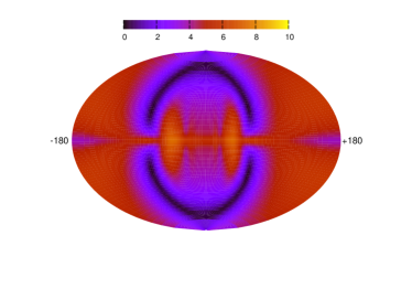
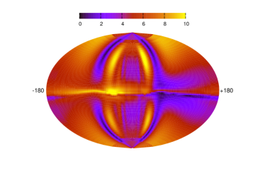
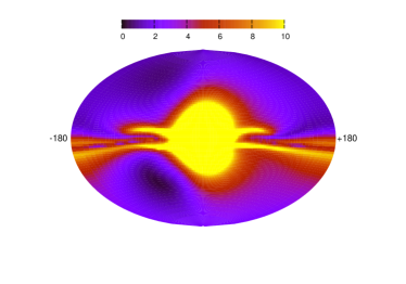
Figure 2: Deflection maps for the TT (top), HMR (middle), and PS (bottom) models of the GMF, for a rigidity of 4$\times$ 10¹⁹ V. The deflection scale is in degree, and the maps refer to the direction as observed at the Earth. All maps use a Hammer-Aitoff projection of Galactic coordinates.

Since we deal with ultra-relativistic particles, the equations of the motion can be written in the form

$$\frac{d{\bf v}}{dt}=\frac{{\bf v}\times{\bf B}}{\cal{R}}\,,$$ (13)

where ${\bf v}$ is a vector of modulus practically equal to $c=1$. The integration is stopped when the particle reaches a distance of 50 kpc from the GC. Note that the energy losses of UHECRs on Galactic scales ($\sim$ 10 kpc) are negligible, provided the trajectory is not very far from a rectilinear one. In Fig. 2, we show the map thus obtained, for the three models considered and a rigidity of $4\times 10^{19}$ V. Note that the deflection $\delta$ of a particle of rigidity $E/Ze$ in a field of strength $B$ coherent over the scale $L$ is approximately given by

$$\delta\simeq 0.53^{\circ}\frac{Z}{E_{20}}\frac{B}{\mu{\rm G}}\frac{L}{\rm kpc}\,.$$ (14)

To obtain an estimate for the average deflection of CRs in different sky regions, labeled as in Table 1, we have followed backwards 50000 randomly chosen CRs of rigidity ${\cal R}=10^{20}$ V, for which the hypothesis of a quasi-rectilinear trajectory is well fulfilled. In Table 2, we show the average value and the square root of the variance of ${\cal R}_{20}\delta$ (i.e., in units of $10^{20}$ V) for the three models of the regular GMF discussed in the Section II, calculated separately for eight different sky regions. The quantity ${\cal R}\delta$ depends only on the GMF model and scales almost linearly with the field strength $B$.

$b_{G}\backslash l_{G}$	315$\,\leq\,l_{G}\,<\,$45	45$\,\leq l_{G}<\,$135	135$\,\leq l_{G}<\,$225	225$\,\leq l_{G}<\,$315
$|b_{G}|\geq\,$30	Ah	Bh	Ch	Dh
$|b_{G}|<\,$30	Al	Bl	Cl	Dl

Table 1: The labels used for the eight different regions of the sky referred to in the text. Angles are in degrees.

The largest difference between the three GMF models occurs in the region Al: in the PS model, the only one with a dipole field, huge deflections arise close to the GC. In the regions Bh, Ch, and Dh the stronger halo fields of the TT and especially the HMR model cause larger deflections than in the PS model. In the l-regions, apart for Al, the deflections of the three models are all of the order $1^{\circ}$–$2^{\circ}$, and comparable to each other within $1\,\sigma$. Since the CR in these directions mainly travel through the disk, in order to escape the Galaxy they have to cross the regions where the field geometry and intensity is better known, and a better agreement among the models exists.

region	${\cal R}_{20}\,\delta$ (PS)	${\cal R}_{20}\,\delta$ (TT)	${\cal R}_{20}\,\delta$ (HMR)
Ah	$1.8^{\circ}\pm 1.0^{\circ}$	$0.9^{\circ}\pm 0.5^{\circ}$	$2.1^{\circ}\pm 0.8^{\circ}$
Bh	$1.3^{\circ}\pm 0.4^{\circ}$	$1.3^{\circ}\pm 0.6^{\circ}$	$2.2^{\circ}\pm 0.8^{\circ}$
Ch	$0.9^{\circ}\pm 0.4^{\circ}$	$2.0^{\circ}\pm 0.3^{\circ}$	$2.7^{\circ}\pm 0.5^{\circ}$
Dh	$0.5^{\circ}\pm 0.2^{\circ}$	$1.1^{\circ}\pm 0.6^{\circ}$	$2.1^{\circ}\pm 0.9^{\circ}$
Al	$14^{\circ}\pm 21^{\circ}$	$1.9^{\circ}\pm 0.4^{\circ}$	$2.2^{\circ}\pm 0.7^{\circ}$
Bl	$2.0^{\circ}\pm 0.9^{\circ}$	$1.7^{\circ}\pm 0.5^{\circ}$	$1.2^{\circ}\pm 0.4^{\circ}$
Cl	$1.7^{\circ}\pm 1.1^{\circ}$	$1.9^{\circ}\pm 0.5^{\circ}$	$1.8^{\circ}\pm 0.3^{\circ}$
Dl	$1.6^{\circ}\pm 1.0^{\circ}$	$1.6^{\circ}\pm 0.5^{\circ}$	$2.3^{\circ}\pm 0.6^{\circ}$

Table 2: The rigidity times average deflections ${\cal R}_{20}\,\delta$ in the eight different regions labeled in Table 1.

If one excludes the central regions of the Galaxy, the average deflection is $\delta\simeq 2^{\circ}/{\cal R}_{20}$, and the differences for the magnitude of the deflections are of the order of 50% among the models. Thus only for the highest energy events and proton primaries the role of the GMF is negligible compared to the angular resolution $\delta_{\rm exp}$ of CR experiments. The latter is as good as $\delta_{\rm exp}\simeq 0.6^{\circ}$ for the HiRes experiment Abbasi:2004ib and for Auger hybrid events AUGERres . For lower ${\cal R}$, correcting for deflections in the GMF would becomes crucial to exploit fully the angular resolution of UHECR experiments. Note also that, even in the ideal case of perfectly known GMF, a reconstruction of the original arrival directions would require a relatively good energy resolution: an uncertainty of, say, 30% in the energy scale around $5\times 10^{19}\>$eV would lead to errors $\gtrsim 1^{\circ}$ in the reconstructed position of proton primaries in most of the sky.

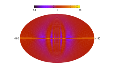
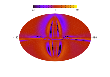
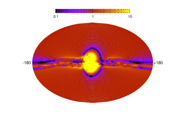
Figure 3: The extragalactic “exposure” maps for the TT (top), HMR (middle), and PS (bottom) model for a rigidity of 4$\times$ 10¹⁹ V. All maps use a Hammer-Aitoff projection of galactic coordinates.

Apart for deflections, (de-) focusing effects of the GMF effectively modify the exposure to the extragalactic sky. This modification can be calculated by back-tracking a large number of events and looking at the obtained map of event numbers per solid angle outside the Galaxy. For the purpose of illustration, we show in Fig. 3 some relative exposure maps obtained for fixed rigidity for the three chosen GMF models. They were obtained with the technique described in Harari:1999it , and essentially represent the ratio $\omega_{B}(l,b)=d\Omega_{\infty}(l^{\prime},b^{\prime})/d\Omega_{\oplus}(l,b)$, where $d\Omega_{\oplus}$ is an infinitesimal small cone at Earth (around the direction $l,b$) transported along the trajectory of a charged particle to the border of the Galaxy $d\Omega_{\infty}$ (around the new position $l^{\prime}(l,b),b^{\prime}(l,b)$). If $\omega_{B}(l,b)$ deviates significantly from one, the corrected exposure has to be used in (auto-) correlation studies. Note how this effect is present in all the models at least for cosmic rays observed at the Earth along the Galactic plane.

A remark on the role of the turbulent GMF is in order. A comparison of Eq. (1) and Eq. (14) shows that deflections in the turbulent GMF are sub-leading. However, this does not ensure automatically that magnetic lensing by the turbulent fields is irrelevant at high energies, because lensing depends on the gradient of the field and the critical energy for amplification is proportional to $L_{c}^{-1/2}$. The detailed analysis of Harari:2002dy showed indeed that small-scale turbulence can produce relatively large magnification effects, and argued that it may even be responsible for (some of) the multiplets seen by AGASA above $4\times 10^{19}$ eV. However, we expect that the random GMF introduces a small scale (and strongly energy dependent) correction of the sky map on the top of the magnification effects of the regular GMF. Then, we argue that neglecting the turbulent GMF in our analysis is justified both for intrinsic reasons and experimental limitations. First, possible lensing effects by the random GMF are weakened by the presence of a regular field component Harari:2002dy : Already without regular field, the magnification peaks are quite narrow in energy space, $\Delta E/E\sim 20\%$, and thus their width $\Delta E/E$ is comparable to the energy resolution of CR experiments. The presence of the regular GMF narrows these magnification peaks further by a factor of several. Due to the limited energy resolutions of current experiments, the turbulent lensing signature would be smeared out. Second, the experimental angular resolution introduces an additional averaging effect. Thus it is seems unlikely that lensing effects of the turbulent GMF lead at present to distinctive effects taking into account the current experimental limitations. Finally, note that from a phenomenological point of view our analysis is the same both if the multiplets are due to intrinsically strong UHECRs sources or due to turbulent lensing.

IV AGASA data sample

In order to make the general considerations of the previous section more concrete, we will discuss here some applications to the AGASA data. The AGASA experiment has published the arrival directions of their data until May 2000 with zenith angle $<45^{\circ}$ and energy above $4\times 10^{19}$ eV AGASA . This data set consists of $N=57$ CRs and contains a clustered component with four pairs and one triplet within $2.5^{\circ}$ that has been interpreted as first signature of point sources of UHECRs. The reconstruction of the original CR arrival directions and the estimate of their errors is obviously an important first step in the identification of astrophysical CR sources.

In Fig. 4, we show the measured directions of all CRs in the AGASA data with $E\geq 10^{20}$ eV together with their reconstructed arrival direction at the border of the Galaxy for the case of Carbon primaries. In the southern Galactic hemisphere, the TT model often produces opposite deflections with respect to the HMR and PS models, because of its antisymmetric field configuration. A longitudinal shift is often appreciable in the PS model, as consequence of the dipolar component we added. The larger deflection found in the TT and HMR models for high latitudes is explained by the stronger regular halo field these models use. The best chances for source identification arise obviously by looking at directions opposite to the GC. On the other hand, observations towards the GC have a certain importance to use the UHECRs as diagnostic tool for GMF, see e.g. TTiy .

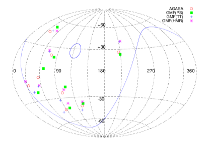
Figure 4: The AGASA data set of CRs with estimated energy exceeding $10^{20}$ eV together with their reconstructed positions assuming Carbon primaries and the three GMF models discussed in the text. The line bounds the region visible to AGASA for zenith angles $\leq 45^{\circ}$; note that for a better visibility, this map is centered around $l=180^{\circ}$, since AGASA is blind to the Galactic Center.

Before turning to the statistical analysis, we briefly recall the estimators we will use in the following. The autocorrelation function $w_{1}$ is defined as

$$w_{1}=\sum_{i=1}^{N_{d}}\sum_{j=1}^{i-1}\Theta(\ell-\ell_{ij})\,,$$ (15)

where $\ell_{ij}$ is the angular distance between the two cosmic rays $i$ and $j$, $\ell$ the chosen bin size, $\Theta$ the step function, and $N_{d}$ is the number of CRs considered. Analogously, one can define the correlation function $w_{\rm s}$ as

$$w_{\rm s}=\sum_{i=1}^{N_{d}}\sum_{a=1}^{N_{\rm s}}\Theta(\ell-\ell_{ia})\,,$$ (16)

where $\ell_{ia}$ is the angular distance between the CR $i$ and the candidate source $a$ and $N_{\rm s}$ is the number of source objects considered.

IV.1 Autocorrelation analysis

Let us discuss now how the small-scale clustering observed by the AGASA experiment is modified by the GMF. Note from Fig. 3 that even for protons the (de-) magnification of the exposure is already significant at energies $4\times 10^{19}$ eV. Neglecting the influence of the GMF (i.e., assuming neutral primaries), one generates a large number of Monte Carlo sets of CRs, each consisting of $N_{d}$ CRs distributed according to the geometrical exposure $\omega_{\rm exp}$ of AGASA. The fraction of MC sets that has a value of the first bin of the autocorrelation function $w_{1}$ larger or equal to the observed one, $w_{1}^{\ast}$, is called the chance probability $P$ of the signal. In the following, we shall consider a bin-width of 2.5^∘, suited for AGASA angular resolution. For a nonzero GMF, one uses the back-tracking method: the observed arrival directions on Earth are back-tracked following a particle with the opposite charge to the boundary of the GMF. Then the value $w$ of the autocorrelation function is calculated. Since also the exposure is changed by the GMF, the CRs of the Monte Carlo sets have to be generated now using as exposure $\omega_{\rm tot}({\cal R},l,b)=\omega_{\rm exp}(l,b)\omega_{B}({\cal R},l,b)$ (the energy spectrum is sampled according to the spectrum observed by AGASA, ${\rm d}N/{\rm d}E\propto E^{-2.7}$). This is automatically fulfilled if one back-tracks uniformly distributed Monte Carlo sets in the same GMF. The resulting chance probability is called $P$ in Table 3. The error due to the statistical fluctuation in the Monte Carlo sets is on the last digit reported. For illustration, we show also the chance probability $P_{0}$ calculated using only the experimental exposure (or $\omega_{B}=1$) that overestimates that clusters come indeed from the same source.

Correcting for the GMF reduces for all three GMF models the value of $w_{1}$. While however for the TT and HMR models two doublets above $5\times 10^{19}$ eV disappear, the PS model loses one low-energy doublet. Thus, either some of the pairs are created by the focusing effect of the GMF, or the GMF and especially its halo component is not well enough reproduced by the models. In the latter case, “true pairs” are destroyed by the the incorrect reconstruction of their trajectories in the GMF. Reference Troitsky:2005bc discussed in detail the effect of the GMF on the AGASA triplet and found that current GMF models defocus it. If the clustering is physical, this could be explained by a wrong modeling of the GMF in that high-latitude region. Alternatively, our assumptions of negligible deflections in the extragalactic magnetic field and of protons as primaries could be wrong. Note that the effect of the GMF induced exposure to the extragalactic sky is not in general negligible. The fact that $P_{0}$ is only somewhat smaller than $P$ hints that only a small fraction of clusters might be caused by magnetic lensing (in the regular field). For the AGASA data set this is expected, because the field of view of this experiment peaks away from the inner regions of the Galactic plane, and the GC in particular. Finally, we note that the energy threshold for which the chance of clustering is minimal decreases for the TT model. This change is however rather small and a larger data set is needed for any definite conclusion.

In Table 4 the same analysis is performed for the TT model only, but assuming also $Z=+2,-1$. In no case is the improvement with respect to the $Z=0$ case appreciable.

Model		no GMF		TT			HMR			PS
$E_{\min}/10^{19}$ eV	$N_{d}$	$w_{1}$	$P[\%]$	$w_{1}$	$P[\%]$	$P_{0}[\%]$	$w_{1}$	$P[\%]$	$P_{0}[\%]$	$w_{1}$	$P[\%]$	$P_{0}[\%]$
5.0	32	4	0.22	2	8.9	8.5	2	9.5	8.5	4	0.27	0.22
4.5	43	6	0.05	4	1.5	1.4	4	1.8	1.4	6	0.10	0.05
4.0	57	7	0.18	6	0.8	0.7	5	3.3	2.4	6	1.09	0.72

Table 3: Number $N$ of CRs with energy $E\geq E_{\min}$ and zenith angle $\theta\leq 45^{\circ}$; the values of the first bin of the autocorrelation function $w_{1}$, and the chance probability $P(w_{1}\geq w_{1}^{\ast})$ from an isotropic test distribution are shown for the two cases with ($P$) and without ($P_{0}$) correction of the exposure, respectively. Proton primaries are assumed.

Model		$Z$=0		$Z$=+1		$Z$=+2		$Z$=-1
$E_{\min}/10^{19}$ eV	$N_{d}$	$w_{1}$	$P[\%]$	$w_{1}$	$P[\%]$	$w_{1}$	$P[\%]$	$w_{1}$	$P[\%]$
5.0	32	4	0.22	2	8.9	1	41	4	0.27
4.5	43	6	0.05	4	1.5	4	1.8	6	0.10
4.0	57	7	0.18	6	0.8	5	3.5	6	1.08

Table 4: As in Table 3, but for different charges of the primary (TT model).

IV.2 Correlations with BL Lacs

Tinyakov and Tkachev examined in Tinyakov:2001ir if correlations of UHECRs arrival directions with BL Lacs improve after correcting for deflections in the GMF (see also otherBL ). The significance of the correlation found is still debated, and we just choose this example as an illustration how correlation of UHECR arrival directions with sources can be used to test the GMF model and the primary charge. We use from the BL Lac catalogue vcv11th all confirmed BL Lacs with magnitude smaller than 18 (187 objects in the whole sky).

Model		no GMF		TT			HMR			PS
$E_{\min}/10^{19}$ eV	$N_{d}$	$w_{\rm bl}$	$P[\%]$	$w_{\rm bl}$	$P[\%]$	$P_{0}[\%]$	$w_{\rm bl}$	$P[\%]$	$P_{0}[\%]$	$w_{\rm bl}$	$P[\%]$	$P_{0}[\%]$
5.0	32	8	8.8	8	9.7	8.8	4	65	64	7	17	17
4.5	43	11	4.7	14	0.6	0.5	7	49	39	7	39	39
4.0	57	13	6.6	20	0.05	0.05	11	20	18	7	67	67

Table 5: As in Table 3, but for the correlation function and the BL Lac catalogue discussed in the text.

In Table 5, we show the chance probability to observe a stronger correlation taking into account the three different GMF models and assuming proton primaries. An improvement of the correlation signal is found only for the TT model, while for the two other models the correlation becomes weaker. In Table 6, the same analysis is performed for $Z=+2$ and $-1$ using the TT model. An improvement with respect to the $Z=0$ case is only found for protons, i.e. for $Z=+1$. Obviously, the two cases $Z=+2$ and -1, i.e. a CR flux consisting only of Helium nuclei or anti-protons, is not expected theoretically, and is used mainly to illustrate the potential of this method to distinguish between different charges. Although it is difficult to draw strong conclusions given present uncertainties, this example clearly shows how UHECRs observations might be used to constrain the GMF models and/or to determine the charge of the CR primaries.

Model		$Z$=0		$Z$=+1		$Z$=+2		$Z$=-1
$E_{\min}/10^{19}$ eV	$N_{d}$	$w_{\rm bl}$	$P[\%]$	$w_{\rm bl}$	$P[\%]$	$w_{\rm bl}$	$P[\%]$	$w_{\rm bl}$	$P[\%]$
5.0	32	8	8.8	8	9.7	7	20	6	27
4.5	43	11	4.7	14	0.6	12	3.4	7	36
4.0	57	13	6.6	20	0.05	13	9.9	8	50

Table 6: As in Table 5, but for different charges of the primary (TT model).

V Conclusion and Perspectives

In this work we have discussed in detail the effect of the regular component of the Galactic magnetic field on the propagation of UHECR, using three GMF models discussed previously in the literature. Both in small-scale clustering and correlation studies, the GMF might be used as a sort of natural spectrograph for UHECR, thus helping in identifying sources, restricting the GMF models as well as the chemical composition of the primaries. Notice that the latter point is an important prerequisite to use UHECR data to study strong interaction at energy scales otherwise inaccessible to laboratory experiments.

As a consequence of the existence of blind regions, we have argued that in some GMF models the observed isotropy of cosmic ray flux e.g. around a few 10${}^{17}\,$eV might disfavor a transition to an extragalactic flux of protons at too low energies, say below 10${}^{17.5}\,$eV. Unfortunately the effect is model-dependent, and a better characterization of the GMF is needed to draw more robust conclusions.

At higher energies, the cosmic rays should enter the ballistic regime. We have provided in tabular and pictorial form an estimate of the typical deflection suffered by UHECRs in the small deflection limit and of its variability from model to model. These results imply that, if the angular resolution of current experiments has to be fully exploited, deflections in the GMF cannot be neglected even for $E=10^{20}\,$eV protons, especially for trajectories along the Galactic plane or crossing the GC region. Since the magnitude as well as the direction of the deflections are very model-dependent, it is difficult to correct for deflections with the present knowledge about the GMF.

We have also emphasized that, to the purpose of statistical analyses like auto-correlation/cross-correlation studies, the GMF can effectively act in distorting the exposure of the experiment to the extragalactic sky, and we provided some maps of this “exposure-modification” effect. As a consequence, to estimate the chance probability e.g. of small-scale clustering, one should take into account the role of the GMF. We showed that this effect is already appreciable in the data published by AGASA, although its field of view do not include the central regions of the Galaxy. Especially for experiments in the southern hemisphere like Auger, one might wonder if excluding some part of the data from (auto-) correlation studies might lead to more robust analyses, at least as long as no reliable model for the GMF is established. We stress that the required cuts would be quite drastic. For instance, fixing $E_{\rm min}=4\times 10^{19}$ eV and considering only sky regions where $|\omega_{B}-1|<0.2$ would exclude

TT: $-5^{\circ}\,<b_{G}\,<\,5^{\circ}$ for all $l_{G}$ and $-60^{\circ}\,<\,b_{G}<\,60^{\circ}$ for $-94^{\circ}<l_{G}<75^{\circ}$,
PS: $-25^{\circ}<b_{G}<22^{\circ}$ for all $l_{G}$ and $-38^{\circ}<b_{G}<40^{\circ}$ for $-33^{\circ}<l_{G}<35^{\circ}$,
HMR: $-11^{\circ}<b_{G}<8^{\circ}$ for all $l_{G}$ and all $b_{G}$ for $-90^{\circ}<l_{G}<90^{\circ}$.

Note that in the HMR model one would cut more than half of the sky. A more reasonable prescription is to evaluate the robustness of the significance of autocorrelation and correlation studies by taking into account several models of GMF and several primary charges, as we have done in this paper for the public available AGASA catalogue. Although the present statistics does not allow to draw strong conclusions, we have not found any signal of improvement after the correction for GMF. This could point to an insufficient knowledge of the field or to a significantly heterogeneous chemical composition of the primaries. Finally, the AGASA signal might only be a chance fluctuation.

Independently on the outcome, performing statistical analyses taking into account several models of GMF and several primary charges is an useful exercise. In the most pessimistic case, it allows one to quantify in an approximate way the contribution of the GMF to the overall uncertainty in the chance probability of a candidate signal. On the other hand, a strong improvement in the significance of a statistical estimator might favor a certain GMF model and/or primary charge assignment. For example, by repeating the study of Tinyakov:2001ir we have found that the significant correlation of BL Lacs with UHECRs is strongly dependent on the GMF and primary adopted, and is present only in the TT model of the GMF for $Z=1$. Although this evidence needs confirmation with a larger data set of UHECRs, it may be the start of the era of UHECR astronomy.

References

- (1) For recent reviews see e.g. M. Nagano and A. A. Watson, Rev. Mod. Phys. 72, 689 (2000); J. W. Cronin, astro-ph/0402487; M. Kachelrieß, Comptes Rendus Physique 5, 441 (2004) [hep-ph/0406174].
- (2) A. A. Watson, Nucl. Phys. Proc. Suppl. 136, 290 (2004) [astro-ph/0408110].
- (3) For an early review see Th. H. Johnson, Rev. Mod. Phys. 10, 193 (1938).
- (4) H. Takami, H. Yoshiguchi and K. Sato, Astrophys. J. 639, 803 (2006) [astro-ph/0506203].
- (5) Y. Uchihori et al., Astropart. Phys. 13, 151 (2000) [astro-ph/9908193]. M. Takeda et al., Astophys. J. 522 225 [astro-ph/9902239]; M. Takeda et al., Proc. 27th ICRC, Hamburg, 2001.
- (6) P. G. Tinyakov and I. I. Tkachev, JETP Lett. 74, 1 (2001) [Pisma Zh. Eksp. Teor. Fiz. 74, 3 (2001)] [astro-ph/0102101]; C. B. Finley and S. Westerhoff, Astropart. Phys. 21, 359 (2004) [astro-ph/0309159].
- (7) H. Yoshiguchi, S. Nagataki and K. Sato, Astrophys. J. 614, 43 (2004) [astro-ph/0404411].
- (8) R. U. Abbasi et al. [The High Resolution Fly’s Eye Collaboration (HIRES)], Astrophys. J. 610 (2004) L73 [astro-ph/0404137].
- (9) M. Kachelrieß and D. Semikoz, Astropart. Phys. 23, 486 (2005) [astro-ph/0405258].
- (10) B. Revenu et al. [The Pierre Auger collaboration], Proc. 29th ICRC, Pune, 2005.
- (11) K. Dolag, D. Grasso, V. Springel and I. Tkachev, JETP Lett. 79, 583 (2004) [Pisma Zh. Eksp. Teor. Fiz. 79, 719 (2004)] [astro-ph/0310902]; JCAP 0501, 009 (2005) [astro-ph/0410419]; G. Sigl, F. Miniati and T. Enßlin, Phys. Rev. D 70, 043007 (2004) [astro-ph/0401084]; Nucl. Phys. Proc. Suppl. 136, 224 (2004) [astro-ph/0409098].
- (12) W. A. Hiltner, Astrophys. J. 109, 471 (1949).
- (13) E. Zwiebel and C. Heiles, Nature 385, 131 (1997).
- (14) R. Stepanov, P. Frick, A. Shukurov and D. Sokoloff, Astron. Astrophys. 391, 361 (2002) [astro-ph/0112507].
- (15) D. Harari, S. Mollerach, E. Roulet and F. Sanchez, JHEP 0203, 045 (2002) [astro-ph/0202362].
- (16) P. G. Tinyakov and I. I. Tkachev, Astropart. Phys.24, 32 (2005) [astro-ph/0411669].
- (17) D. Sokolov, A. Shukurov and M. Krause, Astron. Astrophys. 264, 396 (1992).
- (18) P. Frick, R. Stepanov, A. Shukurov and D. Sokoloff, Mon. Not. Roy. Astron. Soc. 325, 649 (2001) [astro-ph/0012459].
- (19) R. Beck, in ”The Astrophysics of Galactic Cosmic Rays”, eds. R. Diehl et al., Space Science Reviews, Kluwer [astro-ph/0012402].
- (20) R. Beck, A. Brandenburg, D. Moss, A. Shukurov, D. Sokoloff, Ann. Rev. Astron. Astrophys. 34, 155 (1996).
- (21) R. J. Wainscoat et al., Astrophys. J. Suppl. 83, 111 (1992).
- (22) J. Han, in “Astrophysical Polarized Backgrounds”, American Institute of Physics, edited by S. Cecchini et al., p. 96 (2002) [astro-ph/0110319].
- (23) T. Stanev, Astrophys. J. 479, 290 (1997).
- (24) P. G. Tinyakov and I. I. Tkachev, Astropart. Phys. 18, 165 (2002) [astro-ph/0111305].
- (25) R. J. Rand and A. G. Lyne, Mon. Not. Roy. Astron. Soc. 268, 497 (1994).
- (26) K. Beuermann, G. Kanbach, E. M. Berkhuijsen, Astron. Astrophys. 153, 17 (1985).
- (27) J. L. Han, R. N. Manchester, E. M. Berkhuijsen, R. Beck, Astron. Astrophys. 322, 98 (1997).
- (28) J. L. Han, R. N. Manchester, G. J. Qiao, Mon. Not. Roy. Astron. Soc. 306, 371 (1999).
- (29) J. L. Han and G. J. Qiao, Astron. Astrophys. 288, 759 (1994).
- (30) J. L. Han, R. N. Manchester, G. J. Qiao and A. G. Lyne, in ”Radio Pulsars”, APS Conf. Ser., editted by M. Bailes et al. [astro-ph/0211197].
- (31) S. Roy, Bull. Astron. Soc. India 32, 205 (2004) [astro-ph/0411687].
- (32) T. N. LaRosa et al., Astrophys. J. 626, L23 (2005) [astro-ph/0505244].
- (33) D. Harari, S. Mollerach and E. Roulet, JHEP 9908, 022 (1999) [astro-ph/9906309].
- (34) M. Prouza and R. Smida, Astron. Astrophys. 410, 1 (2003) [astro-ph/0307165].
- (35) H. Yoshiguchi, S. Nagataki and K. Sato, Astrophys. J. 596, 1044 (2003) [astro-ph/0307038].
- (36) G. Lemaitre and M. S. Vallarta, Phys. Rev. 43, 87 (1933); W. F. G. Swann, Phys. Rev. 44, 224 (1933).
- (37) J. Alvarez-Muniz, R. Engel and T. Stanev, Astrophys. J. 572, 185 (2002) [astro-ph/0112227].
- (38) M. Ahlers et al., Phys. Rev. D 72, 023001 (2005) [astro-ph/0503229].
- (39) J. Candia, S. Mollerach and E. Roulet, JCAP 0305, 003 (2003) [astro-ph/0302082].
- (40) D. Harari, S. Mollerach and E. Roulet, JHEP 0002, 035 (2000) [astro-ph/0001084].
- (41) S. Karakula, J. .L. Osborne, E. Roberts and W. Tkaczyk, ‘Proc. 12th ICRC (Hobart) 1, 310 (1971).
- (42) C. Bonifazi et al. [The Pierre Auger collaboration], Proc. 29th ICRC, Pune 2005.
- (43) N. Hayashida et al., Astron. J. 120, 2190 (2000) [astro-ph/0008102].
- (44) D. Harari, S. Mollerach and E. Roulet, JHEP 0207, 006 (2002) [astro-ph/0205484] G. Medina-Tanco, M. Teshima, and M. Takeda, Proc. 28th ICRC, Tsukuba 2003; J. Alvarez-Muniz and T. Stanev, astro-ph/0507273;
- (45) S. V. Troitsky, astro-ph/0505262.
- (46) For a discussion of possible correlations of BL Lacs with the HiRes data see D. S. Gorbunov et al., JETP Lett. 80, 145 (2004) [Pisma Zh. Eksp. Teor. Fiz. 80, 167 (2004)] [astro-ph/0406654]; R. U. Abbasi et al. [HiRes Collaboration], Astrophys. J. 636, 680 (2006) [astro-ph/0507120]. The correlation signal between UHECRs and BL Lacs in futute data sets is estimated in D. S. Gorbunov et al., JCAP 0601, 025 (2006) [astro-ph/0508329].
- (47) M.-P. Véron-Cetty and P. Véron, Astron. Astrophys. 412, 399 (2003). The catalogue is available on-line at http://www.obs-hp.fr/www/catalogues/veron2_11/veron2_11.html