Inflation models and observation

Abstract

We consider small-field models which invoke the usual framework for the effective field theory, and large-field models which go beyond that. Present and future possibilities for discriminating between the models are assessed, on the assumption that the primordial curvature perturbation is generated during inflation. With PLANCK data, the theoretical and observational uncertainties on the spectral index will be comparable, providing useful discrimination between small-field models. Further discrimination between models may come later through the tensor fraction, the running of the spectral index and non-gaussianity. The prediction for the trispectrum in a generic multi-field inflation model is given for the first time.

I Introduction

If the primordial curvature perturbation is generated during inflation, observation constrains the height and shape of the inflationary potential. We consider various possibilities for the form for the potential, seeing to what extent present and future observation can distinguish between them. We cover most of the forms that have been proposed, though our citations are far from exhaustive.

In Section II we recall estimates for the number of $e$-folds occurring after the observable Universe leaves the horizon, which has to be specified before a model can be constrained. In Section III we recall the formulas giving the spectral tilt and the tensor fraction generated during single-component inflation. We give the present observational constraints on these quantities as well as future projections, and we plot the region of the $r$-$n$ plane corresponding to small-field models. In Section IV we recall the usual framework for effective field theory, and in V we consider small-field models based on that framework. In Section VI we consider Natural Inflation along with its limiting case $V\propto\phi^{2}$. We also consider the multi-field extension of that case, recalling and extending for that purpose the multi-field formulas for the tilt, the tensor fraction and the non-gaussianity. In Section VIII we see how the models might fare after PLANCK data is available and we conclude in Section IX.

II The number of $e$-folds

Observation provides a direct constraint on inflation only after the observable Universe leaves the horizon. We may call inflation during this era ‘observable inflation’ to distinguish it from the possibly very large amount of inflation occurring earlier. In order to make predictions, we need the number $N(k)$ of $e$-folds of slow-roll inflation, remaining after a scale $k$ leaves the horizon, where $k$ is the coordinate wavenumber corresponding to physical wavenumber $k/a$. The biggest scale of interest is roughly $k=a_{0}H_{0}$ (where $H\equiv\dot{a}/a$ is the Hubble parameter and the subscript denotes the present) and we denote $N(a_{0}H_{0})$ by simply $N$. While cosmological scales leave the horizon we assume almost-exponential inflation giving

$$N(k)=N-\ln(k/a_{0}H_{0}).$$ (1)

To determine $N$ one needs to know something about the history of the Universe between the end of slow-roll inflation and the onset of nucleosynthesis. To be precise, assuming Einstein gravity, one needs the pressure $P$ as a function of the energy density $\rho$. There is also a weak dependence on the value of the Hubble parameter during inflation, equivalent with Einstein gravity to the height of the inflationary potential.

Assume first radiation domination ($P=\rho/3$) from the end of inflation to the onset of nucleosynthesis. Then

$$N = 61-\ln\left(\frac{10^{16}\,\mbox{GeV}}{V^{1/4}}\right)\,.$$ (2)

Here $V$ is the inflationary potential, which for the present purpose can be taken to be constant.

Scales of cosmological interest correspond to

$$0\lesssim\ln\frac{k}{a_{0}H_{0}}\lesssim 14\,,$$ (3)

where the upper limit is the scale enclosing matter with mass $10^{6}M_{\odot}$. They have to leave the horizon during inflation which gives the lower bound $N\gtrsim 14$. Observation requires $V^{1/4}\lesssim 10^{16}\,\mbox{GeV}$ and the onset of nucleosynthesis at temperature $T\simeq 1\,\mbox{MeV}$ requires $V^{1/4}\gtrsim 1\,\mbox{MeV}$, which places the last term of Eq. (2) in the range $0$ to $-40$.

Now we consider other possibilities for $P(\rho)$. The biggest reasonable pressure andrewn is $P=\rho$, corresponding to domination by the kinetic term of a scalar field (kination). If kination dominates from the end of inflation to the onset of nucleosynthesis, the above estimate of $N$ is increased by $\frac{1}{3}\ln(V^{1/4}/1\,\mbox{MeV})<14$. If instead there is matter domination ($P=0$) during that era, the estimate is decreased by the same amount.

Finally, we consider the possibility that significant inflation occurs after slow-roll ends. The most plausible way of arranging this is to invoke one or more bouts of Thermal Inflation thermal , taking place at a relatively low energy scale. Each bout would reduce the estimate $N$ by $10$ or so.

From this discussion, we learn that in principle, $N$ might in principle be anywhere in the range

$$14<N<75\,.$$ (4)

On the other hand, most early Universe scenarios give $0<P<\rho/3$, and most of the models of inflation that we shall discuss give $V$ near the top of its allowed range. In that case, taking $V$ at the very top, we have $47<N<62$ corresponding to

$$N=54\pm 7\,,$$ (5)

and a fractional uncertainty

$$\frac{\Delta N}{N}=0.13\,.$$ (6)

Taking instead $V^{1/4}\sim 10^{10}\,\mbox{GeV}$ (which corresponds to $H\sim\,\mbox{TeV}$ and is the lowest value usually considered) we have $N=34\pm 7$ and a fractional error $\Delta N/N=0.20$.

This discussion leads to a very important conclusion. For any reasonable inflation scale, and post-inflation pressure in the standard range $0<P<\rho/3$, the fractional error in $N$ is of order 10 to $20\%$. As we shall see, the corresponding uncertainties in the predictions are of the same order in a wide range of models.

III Prediction and observation

III.1 Slow-roll inflation

We assume Einstein gravity, and take the fields to be canonically normalized. Until Section VII take the slow-rolling inflaton to have a single component. During inflation, the potential $V(\phi)$ depends only on the inflaton field $\phi$. It is supposed that the field equation

$$\ddot{\phi}+3H\dot{\phi}+V^{\prime}=0$$ (7)

is well-approximated by

$$3H\dot{\phi}=-V^{\prime}\,,$$ (8)

and that the energy density $3M_{\rm P}^{2}H^{2}=V+\frac{1}{2}\dot{\phi}^{2}$ is slowly varying on the Hubble timescale. (We are defining $M_{\rm P}=(8\pi G)^{-1/2}=2.4\times 10^{18}\,\mbox{GeV}$.) These conditions imply

$$3M_{\rm P}^{2}H^{2}\simeq V\,.$$ (9)

and the flatness conditions

$$\epsilon\ll 1\qquad|\eta|\ll 1\,,$$ (10)

where

$$\epsilon \equiv \frac{1}{2}M_{\rm P}^{2}(V^{\prime}/V)^{2}$$ (11)

$$\eta \equiv M_{\rm P}^{2}V^{\prime\prime}/V$$ (12)

Conversely, slow-roll inflation can usually take place on any portion of the potential satisfying the flatness conditions. In the slow-roll approximation $\epsilon$ is slowly varying;

$$H^{-1}\dot{\epsilon}=2\epsilon(2\epsilon-\eta)\,.$$ (13)

For future reference we note that $\dot{\epsilon}$ is positive if $\ln V$ is concave-downward and negative if $\ln V$ is concave-upward.

To obtain the predictions, one needs the field value $\phi(k)$ when a given scale leaves the horizon. From Eqs. (9) and (8) it is related to the number of $e$-folds by $dN(k)/d\phi=M_{\rm P}^{-2}V/V^{\prime}$ and we focus on the biggest scale $k=a_{0}H_{0}$. When this scale leaves the horizon, the field value $\phi_{*}$ is given by

$$N=M_{\rm P}^{-2}\int^{\phi_{*}}_{\phi_{\rm end}}\left(\frac{V}{V^{\prime}}\right)d\phi=M_{\rm P}^{-1}\int^{\phi_{*}}_{\phi_{\rm end}}\frac{d\phi}{\sqrt{2\epsilon(\phi)}}\,,$$ (14)

where $\phi_{\rm end}$ is the value at the end of slow-roll inflation and a star denotes horizon exit for the biggest scale. If $\ln V$ is concave-downward, $\epsilon$ increases with time. Then the value of $N$ will typically be insensitive to $\phi_{\rm end}$, making the model more predictive. The only exception to this rule that arises in practice is the potential $V=V_{0}-\frac{1}{2}m^{2}\phi^{2}$ with $V_{0}$ dominating.

In Figure 1 we plot in the $\log r$-$n$ plane the line $\eta=2\epsilon$, to the left of which $\log V$ is concave-downward, and the line $\eta=0$, to the left of which $V$ itself is concave-downward. For $r\lesssim 10^{-2}$ these lines practically coincide. In Figure 2 we plot the same lines in the $r$-$n$ plane.

In the vacuum, $V=0$. We shall consider both non-hybrid models, where the inflationary value of $V$ is generated almost entirely by the displacement of the inflaton field from its vacuum, and hybrid models where it is generated almost entirely by the displacement of some other (waterfall) field. In non-hybrid models, $\epsilon$ increases with time and inflation ends when one of the flatness conditions fails, after which $\phi$ goes to its vacuum expectation value (vev). In some hybrid models, $\epsilon$ decreases with time ($\log V$ concave-upward), and inflation ends only when the waterfall field is destabilized. In other hybrid inflation models, $\epsilon$ increases with time ($\log V$ concave-downward), and slow-roll inflation may end before the waterfall field is destabilized through the failure of one of the flatness conditions. If that happens, a few more $e$-folds of inflation can take place while the inflaton oscillates about its vev (locked inflation locked ), until the amplitude of the oscillation becomes low enough to destabilize the waterfall field.

III.2 The curvature perturbation

The vacuum fluctuation of the inflaton generates a practically gaussian perturbation, with spectrum ${\cal P}_{\phi}(k)=(H_{k}/2\pi)^{2}$ where the subscript $k$ indicates horizon exit $k=aH$. This perturbation generates at horizon exit a practically gaussian time-independent contribution to the curvature perturbation with spectrum specpred

$${\cal P}_{\zeta}=\frac{1}{24\pi^{2}M_{\rm P}^{4}}\frac{V}{\epsilon}\,.$$ (15)

Subsequently, the perturbations of additional light fields may generate an additional contribution to the curvature perturbation, which come to dominate so that the inflaton contribution is irrelevant. In that case the only constraint on the form of the slow-roll inflaton potential is that Eq. (15) is below the observed value. Here we suppose that instead Eq. (15) gives the dominant value.

Assuming that $\eta$ is slowly varying, the spectral tilt $n-1\equiv d\ln{\cal P}_{\zeta}/d\ln k$ is given by ll92

$$n-1=2\eta-6\epsilon\,.$$ (16)

(We will refer to the tilt $n-1$ instead of to the spectral index $n$ since more direct physical significance.)

In Eqs. (15) and (16) the potential and its derivatives are to be evaluated at horizon exit for the scale $k$ under consideration. We shall evaluate them at the single scale $k=a_{0}H_{0}$, corresponding to $\phi_{*}$ given by Eq. (14). For the forms of the potential that we consider, this is good enough at least with present data. (As we see later future observation might detect the scale dependence of $n$ (running). We are not considering the running mass model, which gives strong running of $n$ that is already constrained by present observations cl ; ourrunning .)

The spectrum is measured with good accuracy as ${\cal P}_{\zeta}=(4.9\times 10^{-5})^{2}$, which with the prediction Eq. (15) requires

$$\frac{V^{1/4}}{\epsilon^{1/4}}=0.027M_{\rm P}=6.6\times 10^{16}\,\mbox{GeV}\,.$$ (17)

At present, measurements of the tilt are consistent with zero. Taking the tensor fraction $r$ to be negligible, which is the prediction of a wide class of models, a fit using WMAP CMB data and the SDSS galaxy survey sdsswmap gives

$$n=0.980\pm 0.020\,.$$ (18)

A fit using instead WMAP CMB data and the 2dFGRS galaxy survey gives 2dfwmap

$$n=0.956\pm 0.020\,.$$ (19)

A fit using WMAP and BOOMERANG CMB data and the SDSS and 2dFGRS galaxy surveys gives wbs2

$$n=0.950\pm 0.020\,.$$ (20)

These bounds are all at 68% confidence level, and all three of them are compatible at this level. For the purpose of illustrating our method we use the results of the first group, for $n$ and also for the tensor fraction that we come to next.

III.3 The tensor fraction

The prediction for the tensor fraction is

$$r=\left(\frac{V^{1/4}}{3.3\times 10^{16}\,\mbox{GeV}}\right)^{4}\,,$$ (21)

which with the cmb normalization (17) is equivalent to

$$r=16\epsilon\,.$$ (22)

Another expression for $r$ involves the field variation. Scales on which the tensor can be observed leave the horizon during about 4 $e$-folds, starting with the exit of the scale $k=a_{0}H_{0}$. During such a brief era $\epsilon$ will be practically constant. From Eqs. (21) and (14), it follows that the variation $\Delta\phi_{4}$ during the four $e$-folds is related to $r$ by mygrav

$$r=\left(\frac{\Delta\phi_{4}}{\sqrt{2}M_{\rm P}}\right)^{2}\,.$$ (23)

If $\epsilon$ is continuously increasing with time ($\log V$ concave-downward), Eqs. (23), (21), and (14) give the strong bound bl ,

$$r<\frac{8}{N^{2}}\left(\frac{\Delta\phi_{N}}{M_{\rm P}}\right)^{2}=0.0032\left(\frac{50}{N}\right)^{2}\left(\frac{\Delta\phi_{N}}{M_{\rm P}}\right)^{2}\,,$$ (24)

where $\Delta\phi_{N}$ is the total field variation. As we remarked earlier, the condition that $\epsilon$ be continuously increasing usually ensures also that $N$ is practically independent of $\phi_{\rm end}$. We shall refer to models with $\Delta\phi_{N}<M_{\rm P}$ as small-field models, and the rest as large-field models.

In Figure 1, the two curved lines divide the $\log r$-$n$ plane into three regions, according to whether $V$ and $\log V$ are concave-upward or concave-downward while cosmological scales leave the horizon. To the right of the rightmost line $\ln V$ is concave-upward while to the left of the leftmost line $V$ is concave-downward. If the concave-upward -downward behaviour persists till the end of slow-roll inflation, the right-hand region is inhabited exclusively by hybrid inflation models, since otherwise inflation would never end.

Still assuming that the concave-upward or -downward characterisation persists after cosmological scales leave the horizon, Figure 1 shows (taking $N=50$) the small-field region defined by $\Delta\phi_{N}<M_{\rm P}$ as well as a reduced small-field region defined by $\Delta\phi_{N}<0.1M_{\rm P}$. (In the right-hand area where Eq. (23) applies, we have assumed that $\Delta\phi_{4}\sim\Delta\phi_{N}$, otherwise the small-field region shrinks.) As we shall see, for inflation models invoking the usual framework of effective field theory, the small-field condition $\Delta\phi_{N}<M_{\rm P}$ usually has to be satisfied by some orders of magnitude. The only exception is if the inflaton is a modulus field, but even there $\Delta\phi_{N}/M_{\rm P}$ is usually well below 1. In Figure 1 we show how the ‘small-field’ region shrinks if it is defined instead by $\Delta\phi_{N}<0.1M_{\rm P}$.

In Figure 2 we repeat the plot of Figure 1 using a linear scale for $r$. This is the plot usually seen in the literature, but it loses important information because a region of very small $r$ is invisible. Following dkk the three regions are usually labeled, from left to right, ‘small-field’, ‘large-field’ and ‘hybrid’, but the first labeling is inappropriate since the bound (24) makes the small-field part of the left-hand region invisible in the linear plot. Also, hybrid models are not confined to the third region.

Now we come to observational constraints involving $r$. If $r$ floats in a fit to data, $n$ should also float since no known inflation model gives negligible tilt with a significant tensor fraction. At present observation gives something like $r<0.5$, $95\%$ confidence level. From Eq. (21) this requires

$$V^{1/4}\lesssim 3\times 10^{16}\,\mbox{GeV}\,.$$ (25)

One can also plot the allowed region in the $r$-$n$ plane. This is shown in Figure 3 for the data analysis that we are using.

Absent a detection, the bound on $r$ will come down dramatically in the future. Data from PLANCK planck will give $r\lesssim 0.05$. Clover clover will give something like $r<10^{-2}$ and the eventual limit may be rlimit something like $r<10^{-4}$. Values of $r$ as low is this have not previously been contemplated in connection with constraints on models of inflation. In the following we will be showing some model predictions in the $\log r$-$n$ plane.

The condition $r>10^{-4}$ for the tilt to be eventually observable is equivalent to $V^{1/4}>3\times 10^{-15}$. As far as the formula (2) is concerned, this is practically at the top of the allowed range. We conclude that for models giving an observable tensor fraction, the estimate (5) of $N$ will hold if $0<P<\rho/3$ between the end of inflation and nucleosynthesis.

Finally, we note that for small-field models, the tilt if it is big enough to observe will be accurately given by

$$n-1=2\eta\,.$$ (26)

This means that for small-field models, the tilt measures the second derivative of the potential. A concave-upward potential corresponds to positive tilt and a concave-downward potential to negative tilt.

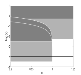
Figure 1: The large-field region corresponding to $\Delta\phi_{N}>M_{\rm P}$ is shaded in dark grey. The region corresponding instead to $\Delta\phi_{N}>0.1M_{\rm P}$ is lightly shaded. To be eventually observable $r$ should be above the black horizontal line.

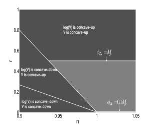
Figure 2: Figure 1 is plotted on a linear scale.

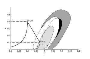
Figure 3: The curved lines are the Natural Inflation predictions for $N=20$ and $N=75$, and the horizontal lines are the corresponding multi-component Chaotic Inflation predictions. The junction of each pair of lines corresponds to single-component Chaotic Inflation. The regions allowed by observation with various assumptions are taken from tegmarketal .

IV Effective field theory

In the usual applications of field theory the relevant scalar fields are close to the fixed point of the relevant symmetries. By ‘close’ we mean that the distance to the origin in field space is much less than the ultra-violet cutoff ${\Lambda_{\rm UV}}$ of the effective field theory under consideration. Starting with some fields and a symmetry group, the action is usually supposed to contain all possible terms not forbidden by the symmetry, including non-renormalizable terms. The coefficients of non-renormalizable terms have by definition negative energy dimension. These coefficients parameterize physics beyond the cutoff ${\Lambda_{\rm UV}}$, and as discussed for instance in weinberg they are usually supposed to be of order 1 in units of the cutoff.

The cutoff presumably cannot be bigger than $M_{\rm P}$. If it is smaller, the effective field theory might be obtained by integrating out some heavy fields in an effective theory with a bigger cutoff. Then a definite contribution to the coefficients of the non-renormalizable terms can be calculated, which hopefully will be dominant. If instead ${\Lambda_{\rm UV}}\sim M_{\rm P}$, there is presently no good way of estimating these coefficients.

The non-renormalizable terms are negligible in most of the usual applications of field theory, but in some situations one or more low-order non-renormalizable terms may be significant. If the presence of some non-renormalizable term is unwelcome, a symmetry might be invoked to forbid or suppress it. Alternatively an argument from string theory or some setup with large extra dimensions might be invoked.

This is the usual setup for effective field theory, normally employed when considering what future colliders and detectors might find as well as in many discussions of the early Universe. Of course one is free instead to write down a lagrangian which does the job in hand without providing any justification for terms which have been omitted (apart from the requirement that they are not effectively generated by quantum effects). That is the view usually taken in for instance discussions of alternative gravity theories involving one or more scalar fields.

Both points of view have been taken in connection with inflation model-building; the usual setup for effective field theory, and the view that the required lagrangian need not be justified. When considering small-field inflation models one usually takes the former, as reviewed for instance in treview ; dl ; bl . Its virtue, here as in other contexts, is that the possibilities for model-building are relatively constrained so that one can exhibit some fairly well-defined examples.

Whichever view one takes, the energy density should be below the cutoff;

$$V^{1/4}<\Lambda_{\rm UV}\,.$$ (27)

In most of the models that we encounter, $V^{1/4}$ is not many orders of magnitude below its maximum value $3\times 10^{16}\,\mbox{GeV}$ which requires that $\Lambda_{\rm UV}$ is not too far below that value. In the context of Einstein gravity $\Lambda_{\rm UV}$ cannot exceed $M_{\rm P}$. Following the usual practice we focus on the maximum value ${\Lambda_{\rm UV}}\sim M_{\rm P}$ which turns out to be advantageous for inflation model-building.

In the effective field theory approach, the tree-level potential is expanded as a power series in the fields keeping only a few low-order terms. If the symmetries relevant for the inflaton are not spontaneously broken, the fixed point lies on the trajectory and $V^{\prime}$ vanishes there. In any case, assuming that $V^{\prime}$ vanishes at some point and choosing that as the origin, the power series expansion for the tree-level potential is

$$V=V_{0}\pm\frac{1}{2}m^{2}\phi^{2}+M\phi^{3}+\frac{1}{4}\lambda\phi^{4}+\sum_{d=5}^{\infty}\lambda_{d}\Lambda_{\rm UV}^{4-d}\phi^{d}\,,$$ (28)

with a symmetry often forbidding all odd terms. The coefficients can have either sign but $\lambda$ and $\lambda_{d}$ are usually taken to be positive and we are adopting the convention that $m^{2}$ is positive. If the non-renormalizable couplings $\lambda_{d}$ are of order 1, we need

$$\phi\ll\Lambda_{\rm UV}\,,$$ (29)

for this series to be under control. Then, barring a cancellation between terms, $V_{0}$ has to dominate and the flatness conditions limit the magnitude of each term.

For the non-renormalizable terms, $|\eta|\ll 1$ with Eqs. (21) and (23) requires treview

$$|\lambda_{d}|\ll 10^{-8}\left(\frac{\Lambda_{\rm UV}}{M_{\rm P}}\right)^{d-4}\left(\frac{3\times 10^{16}\,\mbox{GeV}}{V^{1/4}}\right)^{2(d-4)}\,.$$ (30)

For a given $V$ this constraint is loosest with our adopted value ${\Lambda_{\rm UV}}\sim M_{\rm P}$. It is then compatible with $|\lambda_{d}|\sim 1$ for all values of $d$ for a low inflation scale $V^{1/4}<3\times 10^{10}\,\mbox{GeV}$. More generally it is incompatible with $|\lambda_{d}|\sim 1$ only for the first few values, provided that $V^{1/4}$ is significantly below its maximum possible value. To forbid the first few values one can invoke a discrete symmetry.

For the quadratic and quartic terms, $|\eta|\ll 1$ requires treview (using in the second case also Eqs. (21) and (23))

$$m^{2}M_{\rm P}^{2} \ll V$$ (31)

$$|\lambda| \lesssim 10^{-14}\,.$$ (32)

The second constraint is satisfied in a supersymmetric theory if $\phi$ is taken to be what is called a flat direction. (Flat directions can also be present in non-supersymmetric conformal field theory paul .) Regarding the first constraint, if the mass in a globally supersymmetric theory is set to zero, supergravity generates mass a value

$$m^{2}\sim V/M_{\rm P}^{2}\,,$$ (33)

giving a contribution $|\eta|\sim 1$. That this marginally violates the flatness condition has been called the $\eta$ problem. It may be solved either by modest fine-tuning or by going to a non-generic supergravity theory. More generally, it is possible ewanmulti ; pseudonat to control the mass by making the inflaton a pseudo-Nambu-Goldstone boson.

The condition on the mass becomes problematic if one supposes that the inflaton is a fermion condensate in a generic non-supersymmetric field theory. In such a theory one expects $m$ roughly of order ${\Lambda_{\rm UV}}$, whereas the condition on the mass together with $V<\Lambda_{\rm UV}^{4}$ gives

$$\frac{m^{2}}{\Lambda_{\rm UV}^{2}}\ll\frac{V}{M_{\rm P}^{2}\Lambda_{\rm UV}^{2}}\lesssim 10^{-4}\left(\frac{V^{1/4}}{3\times 10^{16}\,\mbox{GeV}}\right)^{2}\,.$$ (34)

This discussion, based on Eq. (28) with the expectation $|\lambda_{d}|\sim 1$, is appropriate for typical fields. According to string theory there are likely to be special fields (moduli) whose potential is of the form

$$V(\phi)=V_{0}f(\phi/M_{\rm P})\,,$$ (35)

with $f$ and its low derivatives roughly of order 1 at a typical point in the range $0<\phi<M_{\rm P}$. Expanded about a given point, this gives non-renormalizable terms with coefficients of order $\pm V_{0}/M_{\rm P}^{4}$. Taking the point to be a maximum or a minimum so that the expansion has the form (28)

$$m^{2}\sim V_{0}/M_{\rm P}^{2}\,.$$ (36)

In the simplest setup, $m\sim\,\mbox{TeV}$ corresponding to $V_{0}^{1/4}\sim 10^{10}\,\mbox{GeV}$ but that is not supposed to be mandatory.

There is usually supposed to be more than one modulus. If the effective field theory is supersymmetric, the moduli come in pairs (usually taken as components of a complex field) of which one, the ‘axion’ is a PNGB whose potential is periodic with (from Eq. (35)) a period of order $M_{\rm P}$.

V Small-field models

In this section we deal with models of inflation based on the effective field theory approach of the last section. To keep the non-renormalizable terms under control we limit the inflaton field to the range $0<\phi<M_{\rm P}$, making the models automatically small-field models.

V.1 New and modular inflation

We first suppose that inflation takes place near the origin which is a maximum of the potential, as shown in Figure 8. Inflation taking place near a maximum is an attractive possibility because eternal inflation can take place very close to the maximum, providing a natural initial condition for the subsequent slow roll eternal1 ; eternal2 ; bl .

This type of model is usually taken to be non-hybrid, so that the vev ${\langle{\phi}\rangle}$ is the minimum corresponding to $V=0$, and inflation ends with the failure of slow-roll at $\phi_{\rm end}\sim{\langle{\phi}\rangle}<M_{\rm P}$. The reason is that one usually thinks of the maximum as the fixed point of symmetries, which means that one would be dealing with inverted hybrid inflation inverted , as opposed to ordinary hybrid inflation where the field is moving towards a fixed point. Inverted hybrid inflation is more difficult to arrange than ordinary hybrid inflation, especially in the context of supersymmetry. On the other hand, it can be that the origin is not a fixed point, in which case this type of model can be an ordinary hybrid inflation model. To keep things simple we take this kind of inflation to be non-hybrid though the key results still hold if it is hybrid.

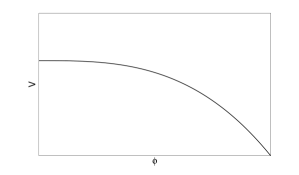
Figure 4: New inflation, modular inflation, etc.

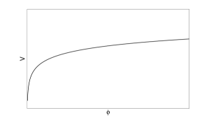
Figure 5: $F$- and $D$-term inflation, mutated hybrid, $D$-branes etc.

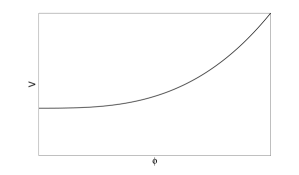
Figure 6: Tree-level hybrid etc.

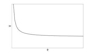
Figure 7: Dynamical supersymmetry breaking, $D$-branes etc.

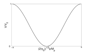
Figure 8: Natural/chaotic inflation

We shall take $\phi_{\rm end}<M_{\rm P}$ to keep within the effective field theory framework of the last section. Since $\Delta\phi_{N}<\phi_{\rm end}$ we then deal with a small-field model, and usually $\Delta\phi_{N}\sim\phi_{\rm end}$.

If ${\phi_{\rm end}}$ is far below $M_{\rm P}$ we shall call this setup New Inflation after the first viable inflation model new . If ${\phi_{\rm end}}$ is not very far below $M_{\rm P}$ we will call it modular inflation, since it is most plausible realised by invoking the potential (35). Modular inflation was discussed for instance in andrei83 ; modular1 ; modular2 ; graham . If there is more than one modulus, modular inflation should take place near a point in the space of the moduli where the potential is an extremum with respect to all of them, which may be difficult to arrange. Also, the trajectory may lie in the space of two or more moduli, corresponding in general to a multi-component inflation model with non-canonical normalization. Here we focus on the case where the trajectory is mainly in the direction of one modulus (taken to be canonically normalized) as for instance in modular2 . (For an example of the opposite case see ks .)

The potential (35) typically gives roughly $\epsilon\sim|\eta|\sim 1$, but the idea is that one gets lucky so that the flatness conditions (10) are marginally satisfied. The extent to which string theory allows modular inflation without fine-tuning is the subject of intense investigation at present, as for example in modular2 .

Considering both New and Modular inflation, let us suppose that one term dominates (28) at least while cosmological scales are leaving the horizon;

$$V=V_{0}\left[1-\left(\frac{\phi}{\mu}\right)^{p}+\cdots\right]\,,$$ (37)

We consider first the case that the dominant term is the leading one;

$$V = V_{0}-\frac{1}{2}m^{2}\phi^{2}+\cdots$$ (38)

$$= V_{0}\left[1-\frac{1}{2}{|\eta_{0}|}\frac{\phi^{2}}{M_{\rm P}^{2}}+\cdots\right]\,,$$ (39)

where $\eta_{0}<0$ is the value of $\eta$ at the maximum. The spectral tilt is $n-1=2\eta_{0}$ so that observation requires ${|\eta_{0}|}\lesssim 0.03$.

To achieve a vev ${\langle{\phi}\rangle}\lesssim M_{\rm P}$, the potential (39) must steepen sharply after cosmological scales leave the horizon. This would be expected for modular inflation (though there is no strong reason to expect the quadratic term to dominate in that case) and it can be arranged for New Inflation as in dr ; pseudonat (see also steve for a hybrid model). As a crude approximation, suppose that the quadratic term dominates until inflation ends at $\phi_{\rm end}\lesssim M_{\rm P}$. Then one finds

$$\phi_{*}=\phi_{\rm end}\exp(-N(1-n)/2)\,,$$ (40)

and bl

$$r=2\left(\frac{\phi_{\rm end}}{M_{\rm P}}\right)^{2}(1-n)^{2}e^{-N(1-n)}\,.$$ (41)

The maximum of this function is below the bound (24) (by a factor $e^{-2}$), consistent with $\log V$ being concave-downward.The prediction $r(n)$ is plotted in Figure 12 for $\phi_{\rm end}=M_{\rm P}$ and $N=50$. Since $\phi_{\rm end}$ is actually expected to be significantly smaller we conclude that $r$ is unlikely to be observable.

This model, with the quadratic term dominating, is reasonable only if $n\lesssim 1-1/N\lesssim 0.98$. Otherwise, from Eq. (40), the quadratic term would have to dominate higher-order terms, up until practically the point where those terms become so important that they steepen the potential causing an immediate end to inflation. Such an abrupt transition is clearly unreasonable in the context of non-hybrid inflation.

All of this assumes that the quadratic term dominates when cosmological scales leave the horizon. The situation is quite different if we assume instead that a higher-order term has become dominant by that time. This case has often been considered as for instance in moreusual , and for modular inflation in graham . Adopting it, we arrive at Eq. (37) with $p\geq 3$. Inflation ends at $\phi_{\rm end}\lesssim\mu$, and to have a small-field model we will take $\mu\lesssim M_{\rm P}$. Then

$$N = \frac{1}{p(p-2)}\left(\frac{\mu}{M_{\rm P}}\right)^{2}\left(\frac{\mu}{\phi_{*}}\right)^{p-2}\left[1-\left(\frac{\phi_{*}}{\phi_{\rm end}}\right)^{p-2}\right]$$ (42)

$$\simeq \frac{1}{p(p-2)}\left(\frac{\mu}{M_{\rm P}}\right)^{2}\left(\frac{\mu}{\phi_{*}}\right)^{p-2}\,.$$

The final equality holds because we are requiring $\phi_{*}/\phi_{\rm end}$ appreciably less than 1, for the reason discussed earlier in connection with the quadratic potential. This gives, independently of $\mu$,

$$n=1-\frac{p-1}{p-2}\frac{2}{N}\,.$$ (43)

The absolute constraint $N<75$ implies $n<0.987$. This prediction is plotted against $N$ in Figure 9 for $p=3$, $4$ and the limiting case $p\to\infty$. We see that $p=3$ is disfavoured by observation, and that for all $p$ observation provides a significant lower bound on $N$. Adopting the reasonable range (5) the prediction becomes

$$n=1-(0.037\pm 0.005)\frac{p-1}{p-2}\,.$$ (44)

This prediction is in the range $n<0.967$.

We have been assuming that a single power in Eq. (37) dominates, which may be unreasonable for modular inflation. But even if a single power does not dominate, Eq. (37) could well be a useful approximation for the relevant values of $\phi$, with some non-integral $p$. Certainly, the specific models of modular2 give the small negative tilt and the high inflation scale which is the characteristic of that approximation. Treating $p>3$ as a continuous variable, the allowed region in the $p$-$N$ plane is shown in Figure 10. Taking $N=54\pm 7$, we plot $n(p)$ in Figure 11.

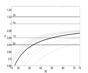
Figure 9: The prediction (43) for different $p$. The bold full line is the limit $|p|\to\infty$. Above it from top down are the lines $p=0$, $-2$ and $-4$, and below it from bottom up are the lines $p=3$, $4$ and $5$. The observational bounds from sdsswmap are indicated.

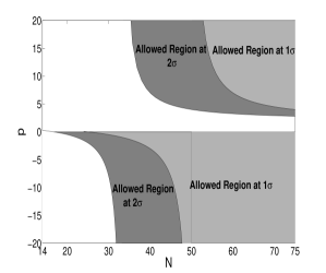
Figure 10: The regions excluded by the observational bounds from sdsswmap , for the parameter $p$ in the prediction (43).

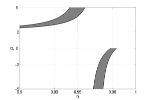
Figure 11: The prediction (43) for $N=54\pm 7$.

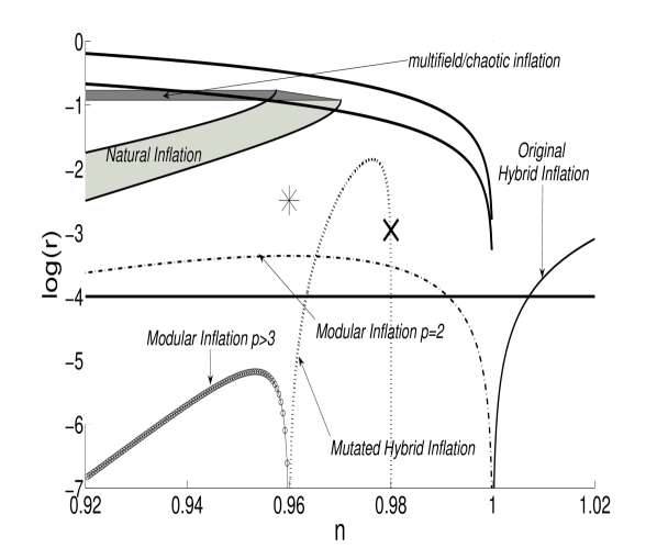
Figure 12: The two upper lines are the ones shown in Figures 1 and 2, which separate the three regimes. The shaded regions give the prediction for natural inflation and multi-component chaotic inflation with $N=54\pm 7$. Single-component chaotic inflation corresponds to the intersection of these two regions. The other predictions are calculated with $N=50$, and they represent upper bounds obtained by setting $\mu$, $\phi_{*}$ or $\phi_{\rm end}$ equal to $M_{\rm P}$, as described in the text. These are the four labeled curves, the cross which corresponds to the $D$/$F$-term potential (46) and the star which corresponds to the exponential potential (50). To be eventually observable, $r$ should be above the horizontal line.

The cmb normalization (17) corresponds to a tensor fraction

$$r=8\left(\frac{\mu}{M_{p}}\right)^{\frac{2p}{p-2}}p^{2}(p(p-2))^{-2\left(\frac{p-1}{p-2}\right)}N^{-2\left(\frac{p-1}{p-2}\right)}\,.$$ (45)

Taking $N=50$, this prediction is plotted in Figure 12 for $\mu=M_{\rm P}$. We see that $r$ is too small ever to observe.

In all of this we focused on the case $p>3$. Allowing instead $p-2$ to be quite small, the first line of Eq. (42) should generally be used. Then, taking $\phi_{\rm end}\simeq M_{\rm P}$, the prediction for $r(n)$ will interpolate between the $p=2$ and $p>3$ curves in Figure 12. As with the quadratic potential, the model makes sense (as a non-hybrid one) only if $n\lesssim 0.98$ since otherwise $\phi_{\rm end}/\phi_{*}$ would be very close to 1.

V.2 $F$- and $D$-term inflation

In a supergravity theory the potential has two parts, called the $F$ term and the $D$ term. They are constructed from three functions, called the superpotential, the Kahler potential and the gauge-kinetic function. There is also a possible constant contribution to the $D$-term called a Fayet-Iliopoulos term. With the simplest (minimal) Kahler potential and gauge-kinetic function, simple forms for the superpotential can be written down which at tree-level are perfectly flat, and can give either $F$-term cllw or $D$-term ewanexp inflation. The loop correction then dominates dss ; dterm , leading to a hybrid inflation model. To ensure that the one-loop correction is a good approximation the renormalization scale $Q$ should be chosen to be of order $\phi$.

In a non-supersymmetric theory the loop correction would generate a term $\lambda\phi^{4}\ln(\phi/Q)$; it was invoked in the original New Inflation model new and it practically corresponds to (37) with $p=4$. In a globally supersymmetric theory with soft supersymmetry breaking, the loop correction corresponds to a running mass term $m^{2}\phi^{2}\ln(\phi/Q)$. Taken as an approximation to supergravity, this gives a running-mass model of inflation ewanrunning , whose observational signature is discussed elsewhere cl ; ourrunning .

The case at hand corresponds (as an approximation to supergravity) to a globally supersymmetric theory with spontaneous supersymmetry breaking, with the loop correction coming from the waterfall field in a hybrid inflation model. Assuming $\phi\gg\phi_{\rm end}$, the potential is

$$V=V_{0}\left[1+\frac{g^{2}}{8\pi^{2}}\ln\frac{\phi}{Q}\right]\,,$$ (46)

where $g\lesssim 1$ is the coupling of $\phi$ to the waterfall field. With $Q\simeq\phi$, $V_{0}$ dominates and $V^{\prime}/V=g^{2}/8\pi^{2}\phi$. The shape of this potential is illustrated in Figure 8. The integral Eq. (14) is again be dominated by the endpoint $\phi_{*}$, so that the tilt is given by Eq. (43) with $p=0$ as $n-1=-1/N$. The observational bound is shown in Figure 9. For this case, the normalization (17) gives a tensor fraction

$$r=\frac{1}{2\pi^{2}}\frac{g^{2}}{N}=0.0011\left(\frac{50}{N}\right)^{2}g^{2}\,.$$ (47)

For $g=1$ this prediction is shown in Figure 12. We see that $r$ will never be observable if $g$ is much below 1.

Although these predictions are clean, they may not be realistic. Even within the setup we have described, there is a regime of parameter space where $\phi$ is close to $\phi_{\rm end}$ so that the coefficient of the log in Eq. (46) is reduced reduce . Much more seriously, the potential (46) gives

$$\phi_{*}=\sqrt{\frac{N}{4\pi^{2}}}gM_{\rm P}\,.$$ (48)

Unless the coupling is very small, this is only marginally a small-field model. A very small coupling is reasonable for the $F$-term case, but not for the $D$-term case.

If the coupling is not very small, the minimal forms for the Kahler and gauge-kinetic functions cannot be justified at all cllw ; mydterm , while the simple form for the superpotential requires an almost exact global symmetry which is usually considered implausible. For these reasons, the tree-level potential is unlikely to be precisely flat in that case. Including it could significantly alter the shape of the potential reduce , possibly generating a maximum bl ; sy . In that case, after re-defining the origin as the maximum, Eq. (37) may be an adequate approximate for some effective $p\gtrsim 3$. In any case, one expects that these $F$- and $D$-term inflation models will give $n<1$ corresponding to a concave-downward potential.

Before leaving $F$- and $D$-term inflation, we remark on their theoretical status. In both cases, the scale of inflation is related to the vev $\Lambda$ of the waterfall field by $V_{0}=g^{2}\Lambda^{4}$, and the cmb normalization determines the latter independently of $g$;

$$\Lambda=\left(\frac{50}{N}\right)^{1/2}\times 6\times 10^{15}\,\mbox{GeV}\,.$$ (49)

(This is equivalent to the fact that Eq. (47) contains a factor $g^{2}$.) In the case of $F$-term inflation, the waterfall field can be identified with a GUT Higgs field. Then $\Lambda$ should be essentially the unification scale deduced from observation, which is $2$ to $3\times 10^{16}\,\mbox{GeV}$. Considering the theoretical uncertainties the agreement is satisfactory, making $F$-term inflation one of the few inflation models which relate the observed value of ${\cal P}_{\zeta}$ to parameters of particle physics. In the case of $D$-term inflation, $\Lambda$ is the normalization of the Fayet-Iliopoulos term. It is related to the string energy scale, but the relation depends on the version of string theory that is relevant rr ; dreview .

V.3 More concave-downward potentials

Next we consider the potential (37), but with $p<0$ to give the shape of Figure 8. Within the context of the setup described in Section IV, this potential can be generated by mutated hybrid inflation mutated ; smooth ; inverted . In mutated hybrid inflation the potential is supposed to have negligible variation in the $\phi$ direction with all other fields fixed at the origin, but there is supposed to be a coupling with some heavy field. At each $\phi$ this field is fixed at the instantaneous minimum of its potential (integrated out), so that the potential $V(\phi)$ during inflation in fact has significant variation. The potential typically is of the form (37) with $p<0$, with integral values of $|p|$ favoured but not mandatory. With integral $p<0$, a potential of the form (37) has also been suggested in $N=2$ supergravity juann2 and in D-brane cosmology dbraneinf .

The predictions are given by the same formulas (43) and (45) as for $p>2$, taking again $\phi$ and $\phi_{\rm end}$ to be sufficiently well-separated. The allowed region in the $p$-$N$ plane is shown in Figure 10. The prediction $n(N)$ is shown in Figure 9 for $p=-1$, $-2$ and $-3$. The observations do not constrain $p$, but they do constrain $N$ significantly. For $N=54\pm 7$ the prediction $n(p)$ is shown in Figure 11. The prediction $r(n)$ with $\mu=M_{\rm P}$ is shown in Figure 12.

Another concave-downward potential is

$$V\simeq V_{0}(1-e^{-q\phi/M_{\rm P}})\,.$$ (50)

This potential has the shape in Figure 8, and it may be generated by a kinetic term passing through zero ewanexp , giving $q=\sqrt{2}$. The same form can arise in non-Einstein gravity inflation treview with $q=\sqrt{2/3}$. This case is actually on the border of the small-field regime, corresponding to $\Delta\phi_{N}\sim M_{\rm P}$, but the kinetic term and the non-Einstein mechanisms both fall outside the framework we set out at in Section IV. The prediction for the spectral tilt is given by Eq. (43) with $p=\infty$ as $n-1=-2/N$. The prediction for $r$ is

$$r=\frac{8}{q^{2}N^{2}}\sim\frac{8}{N^{2}}\,,$$ (51)

which should be observable as shown in Figure 12. A similar form has been derived for the potential of a modulus cq , which gives the same prediction for $n$ but negligible $r<10^{-9}$.

V.4 Concave-upward potentials

Next we consider the original hybrid inflation potential originalhybrid ,

$$V = V_{0}+\frac{1}{2}m^{2}\phi^{2}$$ (52)

$$= V_{0}\left(1+\frac{1}{2}\eta_{0}\frac{\phi^{2}}{M_{\rm P}^{2}}\right)\,,$$ (53)

It is supposed that $\eta_{0}\ll 1$, so that inflation ends only when the waterfall field responsible for $V_{0}$ is destabilized. The constant term $V_{0}$ dominates for $\phi/M_{\rm P}\ll\eta_{0}^{-1}$. In that regime, $\phi_{*}={\phi_{\rm end}}\exp[\frac{1}{2}(n-1)N]$. This gives

$$n-1=2\eta_{0}>0\,.$$ (54)

which might be indistinguishable from $1$. The tensor fraction is

$$r=2\left(\frac{\phi_{*}}{M_{\rm P}}\right)^{2}(n-1)^{2}\,.$$ (55)

Working within the framework of Section IV we need $\phi_{*}<M_{\rm P}$. As shown in Figure 12, the tensor fraction might be observable within this regime.

The original hybrid inflation model makes good contact with field theory beyond the Standard Model. In contrast with the other potentials we consider, the inflation scale $V_{0}$ can be quite low, which would reduce $N$. (Happily, the predictions for the spectral tilt is independent of $N$.) In the context of supersymmetry $V_{0}^{1/4}\sim 10^{10}\,\mbox{GeV}$ is a natural choice supernatural , with $\eta_{0}$ not too small so that $m\sim\,\mbox{TeV}$. The parameter space model is limited however, by the requirement that the loop correction from the waterfall field be negligible myhybrid . Supersymmetric hybrid inflation of any kind is impossible with $V_{0}^{1/4}\sim\,\mbox{TeV}$ which is desirable for instance mytev ; kl in the presence of extra dimensions. (See however clrt for a non-supersymmetric hybrid inflation model with $V^{1/4}\sim\,\mbox{TeV}$, which can generate baryon number as well.)

Next we consider the potential

$$V=V_{0}\left[1+\left(\frac{\phi}{\mu}\right)^{p}+\cdots\right]\,,$$ (56)

with the constant term dominating and $p\geq 2$ or $p<0$. For these values of $p$ the potential has the shape shown respectively in Figures 8 and 8. An integer $p\geq 3$ would correspond andreihybrid ; hybrid2 to a higher-order term dominating, and non-integral values $p>2$ can be motivated as an approximation (cf. the discussion in connection with Eq. (37)) or possibly from mutated hybrid inflation. Negative integral values of $p$ could correspond to dynamical supersymmetry breaking dsb , or to $D$-brane cosmology dbraneinf .

In all of these cases, inflation can occur only in a limited region $\phi<\phi_{\rm max}$, where $\phi_{\rm max}$ corresponds to $\eta\sim 1$, and it is not clear how the field is supposed to arrive in that region. The integral Eq. (14) is dominated by the endpoint $\phi_{\rm end}$ if it is sufficiently well separated from $\phi_{*}$. Then the spectral tilt and tensor fraction are given by Eqs. (43) and (45), with the replacement $N\to N_{\rm max}-N$ where $N_{\rm max}$ is the maximum number of $e$-folds. Barring fine-tuning one expects $N_{\rm max}\gg N$, which probably will make the spectral tilt and the tensor fraction too small to observe.

There remains the case of potentials (37) and (56) in the range $0<p<2$, which looks unlikely in the context of field theory. For the record, if $\phi_{\rm end}$ and $\phi$ are sufficiently well separated, (43) and (45) apply for the potential (56), while for the potential (37) these equations apply with $N\to N_{\rm max}-N$.

VI Single-component Natural/Chaotic inflation

VI.1 The single-component case

Now we consider large-field models, corresponding to $\Delta\phi_{N}>M_{\rm P}$. These lie outside the effective field theory framework described in Section IV.

Most discussions of the large-field case adopt a ‘chaotic inflation’ potential

$$V\propto\phi^{p}\,,$$ (57)

with $p$ an even integer. (The term ‘chaotic’ is used because the potential was first introduced chaotic as the simplest one which would support what Linde called a chaotic initial condition.) With such a potential, $\phi_{*}\simeq\sqrt{2Np}M_{\rm P}$, and $\phi_{\rm end}\sim M_{\rm P}$. With this form of the potential $V^{\prime}/V\propto 1/\phi$ making $\log V$ concave-downward. The integral (14) is practically independent of $\phi_{\rm end}$ leading to the predictions

$$n = -\frac{2+p}{2N}$$ (58)

$$r = \frac{4p}{N}\,.$$ (59)

Observation rules out $p\geq 4$, but marginally allows $p=2$. In Figure 3 we show the prediction for $p=2$, with $20<N<75$. Using the reasonable range (5) it becomes

$$n = -0.037\pm 0.005$$ (60)

$$r = 0.15\pm 0.02$$ (61)

We show this prediction in Figure 12.

Before continuing we address the following point. In a non-supersymmetric theory, where $V$ is part of the lagrangian, one is free to specify the potential (57) even though it goes beyond the effective field theory framework of Section IV. But in the context of supergravity, where $V$ (taking it to come from the $F$ term) has to be constructed from the Kahler potential and the superpotential one might wonder whether a given form is possible at all. That this is so has been demonstrated for $V\propto\phi^{2}$ by writing down explicit forms for the Kahler potential and superpotential adhoc ; kyy ; yy , and similar constructions would surely work for any power. Thus, the status of the potential $V\propto\phi^{p}$ in supergravity is the same as in a non-supersymmetric field theory.

The potential $V\propto\phi^{2}$ may be better motivated if it is considered as an approximation to a sinusoidal potential near a minimum. Such a potential was dubbed Natural Inflation by the people who first considered it natural . To achieve inflation the period of the potential has to be much bigger than $M_{\rm P}$, but proposals have been made extranat ; pseudonat ; Kim:2004rp which motivate such a large period. The first two of these go beyond the framework of Section IV by invoking non-trivial extra dimensions, while the last stays within it by making the field $\phi$ correspond to a path in field space which winds many times around the fixed point.

The sinusoidal potential can be written

$$V=V_{0}\sin^{2}(\sqrt{{|\eta_{0}|}/2}\phi/M_{\rm P})\,,$$ (62)

and is plotted in Figure 8. Provided that ${|\eta_{0}|}\ll 1$, the potential supports inflation until $\eta\sim\epsilon\sim 1$. From Eq. (14),

$$\sin\left(\sqrt{\frac{\eta_{0}}{2}}\frac{\phi_{*}}{M_{\rm P}}\right)\simeq\sqrt{\frac{1}{1+\eta_{0}}}\,e^{-N\eta_{0}}\,,$$ (63)

leading to

$$\epsilon = \frac{1}{2N}\frac{2N{|\eta_{0}|}}{e^{2N{|\eta_{0}|}}-1}$$ (64)

$$\eta = \epsilon-{|\eta_{0}|}\,.$$ (65)

From these expressions one can read off $n-1$ and $r$. At fixed $N$ the prediction depends on the parameter $|\eta_{0}|$. The results for $N=20$ and $N=75$ are shown in Figure 3, and the result for the reasonable range (5) is shown in Figure 12. We see in the latter figure that as $n$ goes more negative we move from the regime $V^{\prime\prime}(\phi_{*})>0$ into the regime $V^{\prime\prime}(\phi_{*})<0$. Note though that the requirement $|\eta_{0}|\ll 1$ always makes this a large-field model ($\Delta\phi_{N}>0$); we see again that the labeling of the left-hand region in Figures 1 and 2 as ‘small-field’ is inappropriate.

VII Multi-component Chaotic Inflation

So far in this paper we dealt only with single-component slow-roll inflation, where the inflationary trajectory is essentially unique; it is either the only possible one in the space of the scalar fields, or else is one of a family of straight-line trajectories which are equivalent during inflation. An important example of the latter case is a potential $V(\phi)$, with

$$\phi^{2}=\sum_{i=1}^{K}\phi_{i}^{2}\,.$$ (66)

We take the $\phi_{i}$ to be canonically normalized, making the radial field $\phi$ also canonically normalized along each direction. Each direction corresponds to a possible inflationary trajectory, but an $SO(K)$ symmetry leaves $\phi^{2}$ invariant and transforms the trajectories into each other.

For a multi-component slow-roll model, there is a family of possible curved trajectories in the space of two or more fields, which we refer to as components of the inflaton. The potential is supposed to satisfy flatness conditions analogous to Eq. (10)

$$\epsilon_{i}\ll 1\qquad|\eta_{ij}|\ll 1\,,$$ (67)

where

$$\epsilon_{i} \equiv \frac{1}{2}M_{\rm P}^{2}\left(\frac{\partial V/\partial\phi_{i}}{V}\right)^{2}$$ (68)

$$\eta_{ij} \equiv M_{\rm P}^{2}\frac{\partial^{2}V/\partial\phi_{i}\partial\phi_{j}}{V}\,.$$ (69)

The field equation for each field $\phi_{i}$ is supposed to be well-approximated by $3H\dot{\phi}_{i}=-\partial V/\partial\phi_{i}$, so that the possible inflationary trajectories are the lines of steepest descent of the potential. The set of all fields satisfying these conditions may be called the set of light fields.

While in principle every field satisfying these conditions could be regarded as components of the inflaton, in practice one will include only those fields corresponding to directions in which the slope $\partial V/\partial\phi_{i}$ is big enough to lead to significant curvature. Light fields corresponding to a smaller slope will have no significant effect during inflation, though they may come into play afterward and be the main source of the curvature perturbation.

To evaluate the curvature perturbation generated by the vacuum fluctuations of the multi-component inflaton, we can use the $\delta N$ formalism starob85 ; ss ; lms ; lr ; st which handles all light fields on an equal footing whether or not they are significant during inflation. Keeping quadratic terms lr , the time-dependent curvature perturbation smoothed on a given comoving scale $a/k$ is

$$\zeta({\mathbf{x}},t) = \delta N(k,\phi_{i}({\mathbf{x}}),\rho(t))$$ (70)

$$= \sum_{i}N_{i}\delta\phi_{i}({\mathbf{x}})+\frac{1}{2}\sum_{ij}N_{ij}\delta\phi_{i}\delta\phi_{j}\,.$$

Here, $N(k,\phi_{i},\rho)$ is the number of $e$-folds, evaluated in an unperturbed universe, from an epoch soon after the smoothing scale leaves the horizon when the fields $\phi_{i}$ have specified values, to an epoch when the energy density $\rho$ has a specified value. In the second line, $N_{i}\equiv\partial N/\partial\phi_{i}$ and $N_{ij}\equiv\partial^{2}N/\partial\phi_{i}\phi_{j}$, both evaluated on the unperturbed trajectory. In known cases the first two terms of this expansion in the field perturbations are enough.

These expressions involve the unperturbed inflationary trajectory. It is not determined by the potential during observable inflation, if more than one field is light then. It may be that well before the observable Universe leaves the horizon there is only one relevant light field, leading to an essentially unique trajectory at the classical level. In any case we suppose that somehow the unperturbed trajectory during observable inflation is known.

To evaluate a given Fourier component of $\zeta({\mathbf{x}},t)$ we can adopt a smoothing scale just a bit shorter than the inverse wavenumber. Thus we may in practice identify $k$ in the above expressions with the wavenumber of the Fourier component.

The field perturbations $\delta\phi_{i}$ are generated from the vacuum fluctuation. They are practically gaussian and uncorrelated, and each of them has the spectrum $(H_{k}/2\pi)^{2}$, where the subscript $k$ denotes the epoch of horizon exit $k=aH$. At some stage before nucleosynthesis, $\zeta$ settles down to a time-independent value, which is constrained by observation. We write down the predictions for $\zeta$, which follow from Eq. (70) at any epoch even though we are interested in the regime where $\zeta$ has settled down to its final value.

Since the observed $\zeta$ is almost gaussian, one or more linear terms must dominate Eq. (70) at least eventually, giving the spectrum

$${\cal P}_{\zeta}(k)=\sum N^{2}_{i}(k)(H_{k}/2\pi)^{2}\,.$$ (71)

Using the multi-component slow-roll formalism the spectral tilt is found to be ss ; treview

$$n-1=-2\epsilon-\frac{2}{M_{\rm P}^{2}N_{i}N_{i}}+2\frac{\eta_{jk}N_{j}N_{k}}{N_{m}N_{m}}\,,\,.$$ (72)

where identical indices are summed over and $\epsilon=\sum_{i}\epsilon_{i}$ is given by Eq. (11) with $V^{\prime}$ the gradient of $V$.

The field basis at horizon exit can be chosen so that one field $\phi$ points along the inflationary trajectory. Its contribution to Eq. (71) is time-independent, and if it dominates the final value one recovers the predictions (15), (16), and (21). The other contributions are initially negligible (almost-exponential inflation being assumed at horizon exit) but may grow to become significant or dominant. The tensor perturbation on the other hand depends only on $H_{k}$ and is time-independent, which means ss ; treview ; book that the tensor fraction cannot exceed the prediction (22);

$$r\leq 16\epsilon\,.$$ (73)

If the contribution of $\phi$ dominates, the non-gaussianity of $\zeta$ is too small to ever be measurable maldacena ; sl . Otherwise it may be observable. The likely observables are the bispectrum and trispectrum, which alone are generated by the quadratic expansion (66). They are specified respectively by bl quantities ${f_{\rm NL}}$ and ${\tau_{\rm NL}}$. Taking the field perturbations to be perfectly gaussian, which has been justified for the bispectrum sl ; lz , and ignoring the scale-dependence of the spectra, the predictions are lr ; bl2

$$-\frac{3}{5}{f_{\rm NL}} = \frac{N_{i}N_{ij}N_{j}}{2\left(N_{m}N_{m}\right)^{2}}+4A{\cal P}_{\zeta}\frac{{\rm Tr\,}N^{3}}{\left(N_{n}N_{n}\right)^{3}}$$ (74)

$${\tau_{\rm NL}} = 2\frac{N_{i}N_{ij}N_{jk}N_{k}}{\left(N_{m}N_{m}\right)^{3}}+16B{\cal P}_{\zeta}\frac{{\rm Tr\,}N^{4}}{\left(N_{n}N_{n}\right)^{4}}\,,$$ (75)

where $A$ and $B$ are of order 1 on cosmological scales. Present observation fnlbound gives roughly $|{f_{\rm NL}}|\lesssim 100$, and absent a detection the eventual bound will be bartolorev $|{f_{\rm NL}}|\lesssim 1$. There is at present no bound on ${\tau_{\rm NL}}$ from modern date, and no estimate of the bound that will eventually be possible. (A crude bound from COBE data bl is $|{\tau_{\rm NL}}|<10^{8}$.)

The shape of the potential of a multi-component inflation model is constrained by these predictions, if $\zeta$ is assumed to have reached its final value by the end of inflation. Stewart and collaborators have exhibited some small-field multi-component models ewanmulti ; ks , along with their prediction for the spectral tilt which depends strongly on the parameters of the potential. We are going to consider instead multi-component chaotic inflation, corresponding to

$$V=\frac{1}{2}\sum_{k=1}^{K}m_{i}^{2}\phi_{i}^{2}\,.$$ (76)

This potential gives uninterrupted slow-roll inflation if the masses are not too unequal interrupt , and we assume that this is the case.

If the field values are of the same order, inflation ends when $\phi_{i}\sim M_{\rm P}/\sqrt{K}\ll M_{\rm P}$, which can be much less than $M_{\rm P}$ if there are many fields. Recalling the discussion of Section IV, one might hope that the potential in that case is generically under good control, with non-renormalizable terms negligible. This general idea was termed Assisted Inflation by those who first considered it assisted . As the authors of Nflation point out, whether this is so should be considered case by case. One can see this by considering the case of equal masses, $m_{i}^{2}=m^{2}$, which gives

$$V=\frac{1}{2}m^{2}\phi^{2}$$ (77)

with $\phi^{2}$ given by Eq. (66) and inflation taking place at $\phi\gg M_{\rm P}$. If this potential were exact, there would be a $SO(K)$ symmetry which would forbid the appearance of non-renormalizable terms $\lambda_{d}\phi_{i}^{d}/M_{\rm P}^{d-4}$; instead there would be terms $\lambda_{d}\phi^{d}/M_{\rm P}^{d-4}$ which presumably would spoil inflation at $\phi\gg M_{\rm P}$ even though the individual $\phi_{i}$ can all be small.

As a specific way of keeping the multi-chaotic potential under control, the authors of Nflation suppose that the potential (76) is actually an approximation to the sum of sinusoidal potentials, evaluated near the minimum of the potential. They called this $N$-flation. Such a potential might arise in string theory, as the sum of the potentials of axions which are components of complex moduli, and it is argued that they are under good theoretical control.

Using the $\delta N$ results, the prediction for Eq. (76) is very simple treview . One finds

$$N(k,\phi_{i},\rho)=\frac{1}{4}\sum\phi_{i}^{2}(k)\,,$$ (78)

independently of the final epoch if it is well after horizon exit. (Remember that $k$ denotes the epoch of horizon exit $aH=k$.) The predictions are

$${\cal P}_{\zeta} = 2N\left(\frac{H}{2\pi}\right)^{2}$$ (79)

$$r = 8/N$$ (80)

$$\epsilon = 2\frac{\sum m_{i}^{4}\phi_{i}^{2}}{\left(\sum m_{i}^{2}\phi_{i}^{2}\right)^{2}}$$ (81)

$$n-1 = -2\epsilon-\frac{1}{N}\,.$$ (82)

The predictions for ${\cal P}_{\zeta}$ and $r$ are the same as in the single-component case. The minimum value of $\epsilon$ at fixed $N$ and ${\cal P}_{\zeta}$ is $1/2N$ and corresponds to equal masses. This reproduces the single-component result $n-1=-2/N$. Making the masses unequal increases $\epsilon$ and one cannot calculate an upper bound on $\epsilon$ without knowing the regime of parameter space within which continuous slow-roll takes place. Hence, making the masses unequal decreases $n-1$ by an unknown amount while leaving $r$ the same. As seen in Figures 3 and 12, this decreases the already-marginal viability of the model when compared with the data that we are using.

Using Eq. (78) one finds that the non-gaussianity parameters ${f_{\rm NL}}$ and ${\tau_{\rm NL}}$ given by Eqs. (74) and (75) are both much less than 1. This means that ${f_{\rm NL}}$ (and presumably also ${\tau_{\rm NL}}$) will never be measurable.

The non-gaussianity parameters have so far been evaluated for just two other multi-component inflation models, those of ks ; ev . Assuming that $\zeta$ attains the observed value by the end of inflation the non-gaussianity is again found to be negligible lr in the case of ks , but it could be significant in the case of ev if the non-gaussian part of the $\zeta$ is generated only after inflation is over lr .

VIII Outlook

With present data the bounds that we have presented are not very restrictive. One sees from Eqs. (18)–(20) that it would be quite reasonable to shift the allowed interval for $n$ down by $0.02$ or so, which would weaken the constraints on models presented in Figure 9. A downward shift in $n$ would also improve the viability of the large-field models presented in Eq. (3).

The situation will change dramatically when the accuracy of the data is improved. Consider first the possibility of discriminating among small-field models, through their prediction for the spectral tilt. Data from PLANCK planck should give kks $\Delta n=\pm 0.007$, reducing to $\Delta n=.003$ with the proposed CMBpol cmbpol . Adding galaxy survey data should give further reduction. Looking at Figure 9, one can distinguish four possibilities, according to the eventual value of $n$.

A value of $n\lesssim 0.98$

This case is very interesting because it is the expected prediction for some of the most reasonable-looking potentials. These are the quadratic potential (39), the potential (37) with $p\geq 2$ (corresponding to new and modular inflation) the same potential with $p<0$ (corresponding to mutated hybrid inflation, some $D$-brane proposals and an $N=2$ supergravity proposal), the $D$/$F$-term potential (46) and the exponential potential (50). Regarding the last two as special cases corresponding to $p\to 0$ and $p\to\infty$ we are dealing with the potential

$$V=V_{0}\left[1-\left(\frac{\phi}{\mu}\right)^{p}\right]\,,$$ (83)

with $\mu\lesssim M_{\rm P}$ and $V_{0}$ dominating.

For $p=2$, the spectral tilt has the scale-invariant value $n=-2V_{0}/M_{\rm P}^{2}\mu^{2}$ provided that this potential is valid on cosmological scales. For all of the other relevant values of $p$ ($p\gtrsim 3$ and $p\leq 0$) we suppose that the potential is valid also for long enough that it gives Eq. (42) for $N$. Then the spectral tilt depends only on $p$, being given by Eq. (43). Adopting the reasonable range Eq. (5), and taking $V^{1/4}\simeq 10^{16}\,\mbox{GeV}$ which for this type of potential is more or less required by the normalization of the spectrum, this prediction becomes

$$n-1=-(0.037\pm 0.005)\frac{p-1}{p-2}\,.$$ (84)

For the allowed range of $p$ the fraction is bigger than $1/2$, and observation requires it to be $\lesssim 2$. We conclude that the theoretical uncertainty in this case is roughly $\Delta n=0.005$, similar to the accuracy promised by PLANCK data.

Since the prediction for $n-1$ is proportional to $1/N$, the predicted running $n^{\prime}\equiv dn/d\ln k$ is

$$n^{\prime}=(n-1)/N=-\frac{p-1}{p-2}\frac{2}{N^{2}},\,,$$ (85)

which will be in the range $-.0004$ to $-.0016$ or so. The expected accuracy kks is $\Delta n^{\prime}\sim 0.003$ from PLANCK and $\Delta n^{\prime}=.0017$ from CMBpol, and galaxy survey data will reduce these uncertainties. It is therefore possible that the predicted running can be verified.

A value $0.98\lesssim n<1.00$.

This will indicate a concave-downward potential. If we are dealing with a non-hybrid model the potential cannot have the simple parameterization (37) ($p>2$ or $p<0$).

A value of $n$ indistinguishable from 1

This would be compatible both with concave-downward hybrid inflation potentials, and with the original hybrid inflation potential $V=V_{0}+\frac{1}{2}m^{2}\phi^{2}$. It would also be compatible with some more complicated models steve ; ks , and the poorly-motivated concave-upward potentials of the form (56).

A value $n>1$

This would favour the original hybrid inflation model $V=V_{0}+\frac{1}{2}m^{2}\phi^{2}$ or its running-mass version ewanrunning . The concave-upward potential (56) could also give $n$ significantly above 1, but not for the most reasonable case $N_{\rm tot}>>N$. A measurement of the running might provide discrimination between these possibilities.

Now consider the tensor fraction $r$. PLANCK planck will give $r\lesssim 0.05$. Clover clover will give something like $r<10^{-2}$ and the eventual limit may be rlimit something like $r<10^{-4}$. We see from Figure 12 that the tensor fraction generated by small-field models is very small. It will not be detectable by PLANCK or Clover, and it will never be detectable if the small-field condition is well-satisfied as would be desirable in the context of the effective field theory framework described in Section IV.

If $r$ is indeed observed by PLANCK or Clover, that would definitely require a large-field model. At present the only large-field models that are under serious consideration and are compatible with observation are Natural Inflation (corresponding to a sinusoidal potential), its limit single-component Chaotic Inflation (corresponding to $V\propto\phi^{2}$) and multi-component Chaotic Inflation.

Natural Inflation corresponds to a line in the $r$-$n$ plane, with an endpoint corresponding to single-component Chaotic Inflation. The same statement applies to multi-component Chaotic Inflation. Single-component Chaotic Inflation corresponds to the point $n=1-2/N$ and $r=8/N$, with $V^{1/4}$ not far below $10^{16}\,\mbox{GeV}$. Using the reasonable range Eq. (5) the predictions become

$$n=-0.963\pm 0.005\qquad r=0.14\pm 0.02\,.$$ (86)

Both $n-1$ and $r$ are proportional to $1/N$, their fractional uncertainties are given by Eq. (6) as roughly $10\%$. Also, their scale dependence is $\propto 1/\ln k$ which might eventually be detectable. To agree with observation the parameters of Natural Inflation and multi-component Chaotic Inflation should be chosen so that the prediction is not vastly different from this one.

Finally, it is worth saying again that any detection of the non-gaussianity parameter $f_{\rm NL}$ would rule out all single-component slow-roll inflation models, as well as multi-component Chaotic Inflation, on the hypothesis that the inflaton perturbation generates the curvature perturbation.

IX Conclusion

In this paper we have surveyed most forms of the inflationary potential, which have some motivation in the context of current ideas about field theory beyond the Standard Model of particle physics. Assuming that the inflaton generates the curvature perturbation, we have seen how observation can constrain the parameters for a given form of the potential, or rule it out.

The approach we are taking may be contrasted with the two other lines of inquiry. One of them reconstruct asks to what extent one may reconstruct the inflationary potential given an essentially unlimited amount of information about the spectrum ${\cal P}_{\zeta}(k)$, and preferably also about the tensor fraction $r(k)$. The other flow generates, using ‘flow equations’ a large family of potentials which can satisfy the data, without reference to current ideas about field theory.