Slitless grism spectroscopy with the HST Advanced Camera for Surveys

Abstract

The Advanced Camera for Surveys on-board HST is equipped with a set of one grism and three prisms for low-resolution, slitless spectroscopy in the range 1150 Å to 10500 Å. The G800L grism provides optical spectroscopy between 5500 Å and $>$ 1 $\mu$m with a mean dispersion of 39 Å/pix and 24 Å/pix (in the first spectral order) when coupled with the Wide Field and the High Resolution Channels, respectively. Given the lack of any on-board calibration lamps for wavelength and narrow band flat-fielding, the G800L grism can only be calibrated using astronomical targets. In this paper, we describe the strategy used to calibrate the grism in orbit, with special attention to the treatment of the field dependence of the grism flat-field, wavelength solution and sensitivity in both Channels.

1 Introduction

Studies of galaxy formation and evolution at high redshift greatly benefit from multi-object spectroscopy, which is widely accessible from the ground. How far in lookback time one can go is, though, severely limited by the emission spectrum of the night sky. This can be overcome with observations from the space, by performing multi-object spectroscopy which turns out to be rather sensitive to compact sources. Indeed, as shown by the GRAPES program (Pirzkal et al. 2004), grism spectroscopy with the HST Advanced Camera for Surveys (ACS) can detect the continuum emission of sources as faint as z${}_{AB}\sim$ 27 in 40 orbits. Multi-object spectroscopy with HST comes with low spectral resolution to compensate for the telescope size, and without slits. As we will discuss in the next Sections, the absence of a slit allows spectra of different sources to overlap, the size of the source to decrease the instrumental spectral resolution and the background to increase since each pixel collects the background emission integrated over the whole spectral range of the dispersing element.

Slitless spectroscopy has been made available with the Hubble Space Telescope (HST) since its launch, in 1990. The first instruments to be equipped with grism/prism elements were the Wide Field Planetary Camera 1 (WFPC1) and the ESA Faint Object Camera (FOC). WFPC1 contained an UV grism (G200L, Horne & MacKenty 1991), covering the spectral range between 1300 Å and 4000 Å with a resolving power of about 100 (at $\lambda$ = 3000 Å) in the first order. The grism was not extensively calibrated in wavelength and flux and was never used for GO science observations. During the time of WFPC1, HST was not yet corrected for spherical aberration.

Two prisms were mounted in the FOC; they covered the spectral ranges 1150 Å $\leq\lambda\leq$ 6000 Å and 1600 Å $\leq\lambda\leq$ 6000 Å with a resolving power R $\simeq$ 100 at $\lambda$ = 1500 Å and $\simeq$ 250 at $\lambda$ = 2500 Å, respectively. They provided slitless, FUV and NUV spectroscopy across the F/96 (14${}^{\prime\prime}\times$ 14^′′) and F/48 (28${}^{\prime\prime}\times$ 28^′′) fields of view. Both prisms were supported modes of FOC, i.e. they were calibrated in wavelength and flux before launch and in-orbit (cf. Paresce & Greenfield 1989, Hack 1992, Hack 1996). Nevertheless, the FOC prisms were seldomly requested by users during the 7 year life-time of this instrument. The FOC prisms were used to address a number of scientific cases, such as the measurement of the UV flux shortward of $\lambda$ = 1800 Å for a sample of QSOs at $z>$ 3 (Jakobsen et al. 1993); the study of the UV morphology and expansion of the SN 1987A ejecta (Jansen & Jakobsen 2001); and to spatially resolve the spectra of the giant stars in the Capella binary system (Young & Dupree 2002).

Since 1997 slitless spectroscopy has become feasible also at infrared wavelengths with NICMOS Camera 3, which is equipped with three grisms (G096, G141 and G206) covering the spectral range 0.8 - 2.5 $\mu$m at a resolving power of $\simeq$ 200 (Noll et al. 2004). While the first two grisms exploit the low background of HST, G206 is subject to the thermal background emission from HST. The three grisms provide multi-object spectroscopy over a field of view of 51${}^{\prime\prime}\times$ 51^′′ at a spatial resolution of 0.2^′′/pix, and were mainly used to study the evolution of field galaxies at 0.7 $<z<$ 1.9 (McCarthy et al. 1999) and to investigate the nature of planets and Kuiper belt objects (McCarthy et al. 1998). During the first two years of NICMOS, the grisms were calibrated in wavelength and flux in orbit, by observing a Galactic Planetary Nebula and a White Dwarf. Software for extracting spectra (NICMOSlook) was released by Freudling & Pirzkal (1997) and Freudling (1999).

The NICMOS grisms have been quite extensively used, by both GO proposals and parallel programs. Prior to the Servicing Mission 3B, the accepted GO proposals requiring spectroscopy represented about 14$\%$ of all the successful NICMOS proposals, while in the case of FOC the approved proposals making use of the prisms amount to only $\simeq$ 4$\%$ of the total.

Although designed as a slit, high-to-medium resolution spectrograph, STIS has also provided slitless spectroscopy mostly with the G750L grating (R $\simeq$ 750 at 7500 Å) when employed in parallel mode. An IRAF routine (SLITLESS in STSDAS/STECF) was developed by N. Pirzkal for the extraction of slitless spectra.

The slitless parallel data of STIS have been analyzed to search for new low-mass stars and brown dwarfs (Plait 1998a and 1998b), to study the intermediate-redshift Universe (de Mello & Pasquali 2001, Teplitz et al. 2001, Teplitz et al. 2003) and to derive the hydrogen reionization edge (Windhorst et al. 2000).

In March 2002, HST was refurnished with a new instrument, the Advanced Camera for Surveys (ACS) which offers the unique combination of a large field of view (3^′.4 $\times$ 3^′.4) with a high angular resolution (0.05^′′/pix, cf. Sect. 2). The main task of ACS is to perform deep imaging and spectroscopic surveys. In contrast to older generation instruments, the ACS grism and prisms have been extensively calibrated in laboratory and specific GO calibration proposals have been set up to assess their in-orbit performance. It is believed that such an effort will involve a larger number of HST users in using the ACS spectroscopic capabilities and will return relevant scientific results. In the first two years of ACS, the grism has been extensively used for the search for supernovae type Ia at high redshift (Magee et al. 2002, Tsvetanov et al. 2002, Blakeslee et al. 2003, Riess et al. 2004) and for high-redshift Ly$\alpha$ emitters, and to study galaxy formation and evolution at intermediate-to-high redshifts, especially in the UDF field (Pirzkal et al. 2004,2005a,b; Xu et al. 2005; Daddi et al. 2005; Malhotra et al. 2005; Pasquali et al. 2005a,b; Rhoads et al. 2005).

In this paper, we review the concepts and technique of the grism calibrations, which have been developed for non-drizzled, geometrically distorted data. Drizzling the grism data, before establishing their dispersion solution, involve a change of pixel size and geometry which in turn affect the dispersion and zero point of the wavelength calibration and also the amplitude and wavelength dependence of the flat-field correction for grism spectra. These quantities depend on the drizzle parameters which can be specified differently each time by different users. For these reasons, the grism calibration has been performed only for raw grism data.

2 The ACS instrument layout

The ACS is a three-channel instrument which performs broad and narrow band filter imaging from UV to NIR, polarimetric imaging at ultraviolet and optical wavelengths, and low-resolution slitless spectroscopy in the range from $\simeq$ 1150 Å to $\lambda$ $\simeq$ 1 $\mu$m with a set of grism and prisms (cf. http://www.stsci.edu/hst/acs/documents). The ACS spectral elements can be summarized as follow:

The Wide Field Channel (WFC) has a 3^′.4 $\times$ 3^′.4 field of view at a spatial resolution of 0.05^′′/pix and is equipped with a grism (G800L) covering the spectral range from 5500 Å to 1 $\mu$m with a response peak at $\simeq$ 7200 Å and $\simeq$ 6000 Å  in the 1^st and 2^nd orders, respectively. The grism resolving power is $\simeq$ 100 and the dispersion is nearly linear, $\simeq$ 39 Å/pix in the 1^st order and $\simeq$ 20 Å/pix in the 2^nd order. The tilt of the spectra is nearly -2^o from the image X axis, varying slightly across the field.

The High Resolution Channel (HRC) is characterized by a 26${}^{\prime\prime}\times$ 29^′′ FOV with a spatial resolution of 0.027^′′/pix and uses the same grism of the WFC, which introduces a tilt in the spectra of -38^o (from the image X axis) and offers a dispersion of $\simeq$ 24 Å/pix in the 1^st order and of $\simeq$ 13 Å/pix in the 2^nd order. The HRC also features a prism (PR200L) covering the 1600 - 5000 Å range, with a non linear dispersion varying from 2.6 Å/pix at 1600 Å to 105 Å/pix at 3500 Å and 560 Å/pix at 5000 Å.

The Solar Blind Channel (SBC) has a field of view of 31${}^{\prime\prime}\times$ 35^′′ where each pixel is 0.032^′′ in size. Two prisms are available with the SBC: PR110L covering from 1150 Å to 2000 Å, and PR130L from 1220 Å to 2000 Å(i.e. geocoronal Ly$\alpha$ is blocked). The dispersion of PR110L is 2.6 Å/pix at 1216 Å, while the dispersion of PR130L varies from 1.65 Å/pix at 1250 Å to 20.2 Å/pix at 1800 Å.

The ACS grism and prisms are used in slitless mode. This raises a number of important issues:

i) The extension of a source along the dispersion axis is given by the spatial profile of the object, and affects the achievable spectral resolution.

ii) The zero point of the grism wavelength calibration is defined by the position of the object in the direct image. When no direct image of the source is available, the position of the 0^th order can also be used, though in a less accurate way since the 0^th order is itself dispersed.

iii) The spectroscopic flat-field is field and wavelength dependent. Depending on the position of a target in the direct image, the same pixel in the grism/prism image receives different wavelengths.

iv) Each pixel in a grism/prism spectrum has a contribution from the background emission which is integrated over the entire spectral range of the grism/prism.

v) Depending on the luminosity of a source, the grism orders higher than 1 (at higher X coordinates in the grism image) and the grism negative orders (at lower X coordinates) can be identified. No filter can be used to suppress higher and negative orders.

vi) Depending on the position of the object in the direct image, the source spectrum can be truncated in the grism/prism image. Objects outside the field of view can still produce spectra in the grism/prism image.

vii) The extension of grism spectra and the number of their orders can give overlap and contamination among spectra of adjacent objects.

Therefore, the wavelength calibration of the ACS grism and prisms requires a full description of the grism/prisms physical properties, such as the tilt of the spectra, the length of the prism spectra and of the grism orders together with their separation from the grism 0^th order, the (X,Y) offsets between the object position in the direct image and the corresponding 0^th order in the grism image. Indeed, these quantities allow the identification of the spectrum in the grism/prism image of any object in the direct image, the tracing of spectra and set the size of the aperture extraction for each prism spectrum and grism order (Pasquali et al. 2003a,b). As described in the next Sections, these parameters are field-dependent because of the geometric distortions of ACS. This is also true for the flat-field, which an accurate flux calibration of the spectra depends on.

3 The effective spectral dispersion of the ACS grism

Since no slit is available, the nominal dispersion of the ACS grism gets convolved with the object size and, in the case of non-round sources, with the object size along the dispersion axis as determined by the object orientation. This convolution obviously lowers the grism resolution and plays a key role in planning the spectroscopic calibrations and the GO observations with the ACS (Pasquali et al. 2001a).

To quantify the effect of object size and orientation on the effective dispersion of the grism, we have simulated the optical spectrum of the Galactic Planetary Nebula NGC 7009 using SLIM 1.0 (Pirzkal & Pasquali 2001, Pirzkal et al. 2001b). SLIM 1.0 is a slitless spectroscopy simulator developed by N. Pirzkal and is designed to produce realistic and photometrically correct spectra acquired with the ACS grism and prisms. Briefly, any input spectrum is redshifted as required and scaled to a desired magnitude in a reference filter, then dispersed according to the grism/prisms dispersion solution. At each wavelength, the dispersed spectrum is convolved with the grism/prisms throughput curve and with a gaussian PSF whose FWHM value is set by the HST diffraction limit at any specific wavelength.

Two sets of simulations have been produced for both the WFC and the HRC which do not include background or read-out noise. The first set is based on the assumption that NGC 7009 is disc-shaped, with uniform surface brightness and diameter varying from 0^′′.05 to 0^′′.1, 0^′′.4 and 1^′′ for the WFC, and from 0^′′.06 to 0^′′.2 and 0^′′.5 for the HRC. The second set assumes that NGC 7009 is elliptical with a varying position angle (PA) with respect to the dispersion axis. The nebula size is 0^′′.1 $\times$ 0^′′.25 and 0^′′.05 $\times$ 0^′′.12 for the WFC and the HRC respectively. The PA of the nebula major axis is assumed to vary from 0^o to 20^o, 45^o and 90^o so that the object major axis progressively goes from being aligned along to being perpendicular to the dispersion axis.

We have measured the FWHM of a few lines in the 1^st and 2^nd order spectra obtained for the WFC and the HRC in both sets of simulations, in order to quantify the degradation of the grism nominal dispersion as a function of object size. These FWHM values have been normalized to the FWHM of a source with a 0^′′.05 diameter and are plotted in Figure 1 as a function of the object size along the dispersion axis in arcsecs, for both the WFC and the HRC. As expected, the line FWHM nearly doubles by doubling the object linear size, implying that the grism dispersion degrades by almost the same factor as the object size increases. The flattening in the curves for linear sizes larger than 3 $\times$ 0^′′.05 for the WFC (3 $\times$ 0^′′.03 for the HRC) is due to severe line blending which makes the line width measurements unreliable.

4 The calibration strategy

4.1 Ground calibrations

During the ground testing of ACS at the Goddard Space Flight Center, the Refractive Aberration Simulator (RAS/RAMP) was used to acquire a series of grism spectra for both the WFC and the HRC. Specifically, spectra were obtained through a 4 $\mu$m pinhole aperture fed by an Argon lamp and QTH fiber lamp sources. Spectra were acquired at different positions across the field of view, located close to the center and to the CCD amplifiers in the corners. These data provided a first wavelength calibration, and also allowed to check the amplitude of the field dependence of the grism resolution. The spectra of the continuum lamp were used to derive the relative, integrated throughput of the different grism orders across the field of view, but were not suited to determine the throughput as a function of wavelength for the various grism orders. We could then establish that the total power in the 0^th order is 2.5$\%$ of that in the 1^st order, and 1$\%$ and 0.5$\%$ in the positive and negative higher orders, respectively.

Since the grism is sensitive to wavelengths redder than 5500 Å, we could identify and use only the Argon lines redward of 6700 Å. This made the wavelength solutions of the grism orders less accurate than those derived in orbit (cf. Sects. 9 and 10). For example, the wavelength solution of the positive 1^st order could only be fitted with a first-order polynomial, which, later on, gave raise to significant wavelength offsets in the spectra of the in-orbit calibrators.

4.2 In-orbit calibrations

The results obtained in Sect. 3 pose important constraints on the planning of wavelength calibration observations, such as those foreseen for the Servicing Mission Orbital Verification (SMOV, following the installation of ACS onboard HST) tests and subsequent GO calibration programs. ACS is not equipped with arc lamps, therefore the in-orbit dispersion correction of the grism can only be determined from observations of specific astrophysical sources. For this purpose, calibration targets should satisfy the following requirements:

i) the spatial extension of the target should be minimal, to allow accurate determination of the dispersion and wavelength zero point;

ii) the target brightness allows for reasonably short exposure times;

iii) the target spectra should contain a significant number of unblended emission lines;

iv) no extended nebulosity is associated with the targets which would degrade the dispersion of the instrument and increase the local background;

v) the spectrophotometric variability (either intrinsic or induced by an eclipsing companion or by orbital motion) is negligible so that emission features can be identified at the same wavelength at any observational date;

vi) the targets should not lie in crowded fields to avoid contamination by nearby spectra.

Spectroscopy in slitless mode relies on a pair of direct and grism images, since the zero point of the grism wavelength solution is set by the position of the object in the direct image. Because the ACS is tilted with respect to the optical axis of HST, its field of view suffers severe geometric distortions which introduce a field dependence in the grism dispersion and wavelength zero point. Hence, calibration targets have to be observed at a number of positions across the WFC and HRC chips in order to be able to parameterize the field dependence of the grism wavelength solution. This need strengthens requirement i): the exposure times for the calibration targets should be reasonably short to allow multiple acquisitions across the field of view.

In what follows, we discuss the observational strategy adopted for the SMOV tests and following GO calibrations in order to achieve the wavelength calibration of the ACS grism.

4.3 The traditional calibrators: Planetary Nebulae

At optical wavelengths, the spectra of Planetary Nebulae are dominated by strong, narrow emission lines mainly due to H, HeI, [O II], [N II], [O III] and [S III]. The [O III] and [ NII] lines are often used to measure the expansion velocity of Planetary Nebulae (PNe); Galactic PNe span a wide range in expansion velocities, from $\sim$ 5 km s^-1 to 50 km s^-1 (Acker et al. 1992). In the worst case, an expansion velocity of 50 km s^-1 corresponds to a FWHM value of $\sim$ 1 Å at the restframe H$\alpha$ line. With a resolving power of R $\simeq$ 100, the ACS grism does not resolve any Planetary Nebula in velocity and any Planetary Nebula would be equivalent to a ground arc lamp. Among all the known PNe, only those which are compact (with a full size smaller than 0.1^′′) can be observed with the ACS grism according to the requirements listed in Sect. 4. PNe in the Galaxy and in the Magellanic Clouds are rarely compact when imaged with HST and even when compact often have a low intensity halo. Therefore, in order to preserve the nominal dispersion of the ACS grism, we have to resort to more distant PNe, for example those in M31.

To assess the feasibility of grism observations of extragalactic PNe in terms of exposure time and S/N ratio in the lines, we simulated the ACS spectra of the brightest and most compact PNe in M31 using SLIM 1.0 (cf. Pasquali et al. 2001b). The selected PNe were originally studied by Ciardullo et al. (1989) and Jacoby & Ciardullo (1999). Our simulations show that PNe can be used to determine the dispersion correction of the grism 1^st order, but fail the wavelength calibration of the 2^nd since only two lines can be detected with a reasonable S/N ratio. To improve this, the integration time should be longer by a factor of $\sim$3 (equivalent to $\sim$ 1 h per pointing), thus making PNe too time-consuming for routine GO calibration programs. An additional disadvantage of observing PNe in M31 is the field crowding, which makes spectra of adjacent sources overlap. Nevertheless, PNe can be employed as secondary targets, to verify the accurateness of the wavelength calibration.

4.4 An alternative choice: Galactic emission line stars

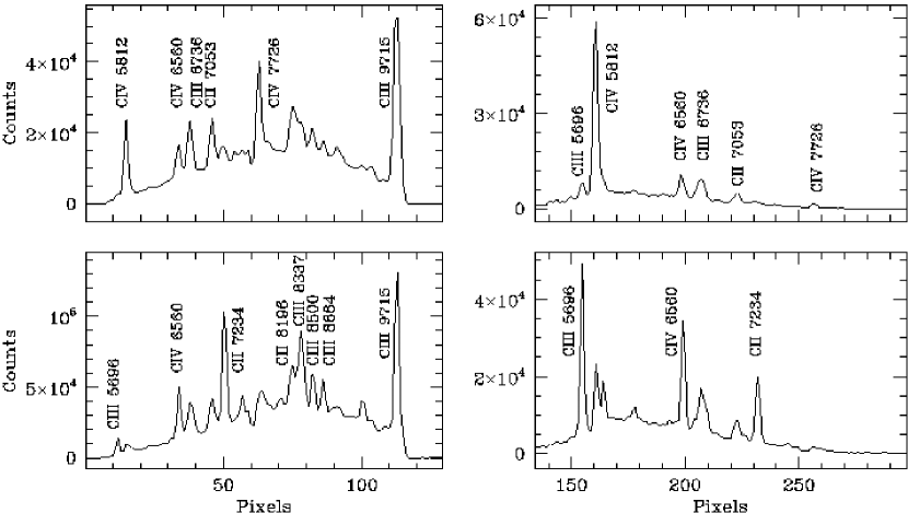
Figure 2: The SLIM WFC spectra for WR stars of spectral template WC6 (top) and WC8 (bottom). First orders are plotted in the left column and refer to an exposure time of 10 s. The second order spectra are shown in the right column and have been computed for an integration time of 60 s.

Having discharged PNe, our simulations show that Galactic Wolf-Rayet (WR) stars satisfy the calibration requirements. As Figure 2 points out, WR stars of spectral type WC6 - WC9 have a large number of bright emission lines (He and C) in the spectral range covered by the ACS grism. The only drawback here is that the velocity of their stellar winds considerably broadens their emission features.

The known Galactic WR stars (van der Hucht 2001) have wind velocities between $\sim$ 700 km s^-1 and 3300 km s^-1 with a mean wind speed of about 1700 km s^-1 and with 19$\%$ of the sample having a wind velocity larger than 2100 km s^-1. We thus assumed a wind speed of 2000 km s^-1 and computed the line broadening induced in WFC and HRC grism spectra of WR stars. The results indicate that such a stellar wind is hardly resolved in the 1^st order spectra and partially affects the 2^nd order spectra. Higher wind velocities rapidly decrease the grism resolution at any order.

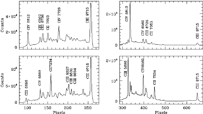
Figure 3: As in Figure 2 but for the HRC. First orders are plotted in the left column and refer to an exposure time of 20 s. The second order spectra are shown in the right column and have been computed for an integration time of 60 s.

Clearly, the wind velocity constraint ($v_{\infty}\leq$ 2000 km s^-1) has to be added to the selection criteria discussed earlier in Sect. 4, together with the requirement that the variability of the selected targets is negligible. Spectro-photometric variability could change the number of detectable emission lines, and variability in the stellar wind could change the line FWHM; both cases would make the grism wavelength calibration less accurate. From the catalogue of van der Hucht (2001), we have selected two stars, WR45 and WR96, whose spectral type, coordinates, V magnitude and wind velocity are listed in Table 1. We produced SLIM 1.0 spectra based on two WR templates kindly provided by P. Crowther and closely matching the spectral types of WR45 and WR96. The simulations are plotted in Figures 2 and 3 for the WFC and the HRC 1^st and 2^nd orders, respectively. In the case of the WFC simulations, an exposure time of 10 s and 60 s has been assumed for the 1^st and 2^nd order, respectively, while for the HRC 20 s and 60 s. Contrary to the Planetary Nebula case, the simulated spectra of WR45 and WR96 indicate that a relatively large sample of emission lines can be used for the wavelength calibration of both the 1^st and 2^nd orders of the ACS grism.

As a counter-check, the simulated spectra of WR45 and WR96 have been used to derive the grism wavelength solution for both the WFC and the HRC. We have measured the position of each identified line in the SLIM output in pixels scaled to the position of the object in the direct image, and fitted pixels against wavelength assuming a first order polynomial. The accuracy of the dispersion correction thus obtained is better than 0.3 pixels for both the 1^st and 2^nd order (i.e. 12 Å and 7 Å, respectively).

4.5 ESO/NTT support observations of WR45 and WR96

Since no high resolution spectra were available in literature at the time of the ACS ground calibrations, we observed WR45 and WR96 with the EMMI spectrograph, mounted on the ESO NTT telescope (266.D-5653, PI Pasquali). The observations were performed in service mode in June and August 2001 as part of the ESO Director General Discretionary Time. Spectra were acquired through the REMD grating $\#$ 8 (between 5000 and 7500 Å at 1.26 Å/pix, and in the range 7300 - 9750 Å at 1.26 Å/pix) and the RILD grism $\#$ 2 (from 4000 to 9000 Å at 2.7 Å/pix). The high resolution spectra were used for an accurate identification of the He and C lines typical of WR stars, while the low resolution spectra provided the flux calibration of the stellar continuum and lines. The NTT, high resolution spectra of WR45 and WR96 are plotted in Figure 4. They were used as inputs to SLIM 1.0 in order to simulate the WFC and HRC grism observations of WR45 and WR96 and to optimize the exposure time and S/N value of the in-orbit calibrations.

5 The ACS observations of WR45 and WR96

As part of the SMOV and INTERIM calibration programs (9029 and 9568, PI Pasquali), we observed WR45 at a number of positions across the field of view of the WFC and the HRC. WR96 was also observed, but only with the WFC, at the same positions used for WR45. We selected 10 pointings for the WFC (among which the five from the ground tests) and 5 (only those observed during the ground calibrations) for the HRC, in order to sample the field dependence of the grism properties, which ground-based calibrations indicated to be smaller for the HRC. WR96 was re-observed in Cycle 12 together with the Planetary Nebula SMP-81 in the LMC (Program 10058, PI Walsh). These observations were designed to provide additional sampling points across the field of view to better map the spatial variation of the wavelength solution. The INTERIM, and Cycle 12 data (i.e. the object positions in the direct image) are illustrated in Figures 5 and 6.

At each pointing a pair of direct and grism images was acquired and repeated at least twice, either during the same visit or in different visits, to test the repeatability of the filter wheel positioning. Direct images were taken with the F625W and F775W filters to test whether the target position in the direct image is filter-dependent. Exposure times for imaging and spectroscopy are listed in Table 2 for both Channels and targets. In particular, the spectroscopic exposure times were tuned to get a S/N ratio $\geq$ 30 in both the positive and negative 1^st and 2^nd orders, and turned out to be long enough to detect the 3^rd and -3^rd orders.

The observations included also two White Dwarfs, GD 153 and G191B2B, which were acquired at the same positions across the chips as the WR stars. Their spectra were used to derive the grism throughput and flux calibration of the WFC and the HRC grism configurations.

6 The WFC/grism configuration

The spectral tilt can be derived from the (X,Y) coordinates of the line-emission peaks, as measured along the spectrum from the -3^rd to the +3^rd order in the grism spectra. We have fitted up to 20 (X,Y) pairs with a first order polynomial, whose slope is the tilt of the grism spectra with respect the X axis of the grism image.

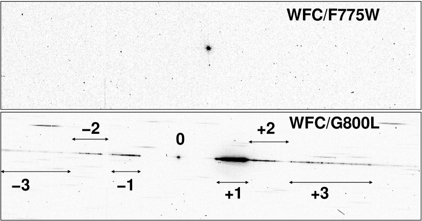
Figure 8: The 2D grism spectrum of WR96 taken with the WFC (bottom panel), where seven orders, from the negative to the positive third, have been identified. The upper panel shows the position of the object in the direct image at which the grism spectrum was acquired. The size of both images is 1500 $\times$ 400 pixels.

On average, the spectral tilt in the WFC/grism configuration is 1^o.98 $\pm$ 0^o.34 from the image X axis, but it varies by 1^o across the field of view of the WFC (cf. Figure 8). The maximum variation ($\sim$ 1^o.1) occurs along the diagonal from the top left corner to the bottom right; a variation of 0^o.79 is seen along the diagonal from the bottom left to the top right corner of the field of view (cf. Pasquali et al. 2003a).

The spectra appear off-set from the object in the direct image. We measured the positions of the 0^th order and the object in the direct image using their light centroid. We used the fits of the spectral tilt to calculate the Y^′ coordinate on the spectrum corresponding to the X coordinate of the object in the direct image. The difference (Y${}_{0^{th}}$ - Y^′) represents an offset between the object in the direct image and the grism 0^th order, which allows to locate the spectrum of a source in the grism image once the source coordinates have been measured in the direct image.

The mean value of this Y-offset across the field of view is -3 pixels, although the Y-offset is itself field dependent. The offset of the object in the direct image from the grism 0^th order along the X axis is almost constant across the WFC field of view and is of about 112 pixels (cf. Pasquali et al. 2003a and Figure 8).

To estimate the length of the grism orders along the image X axis, a threshold has to be set in the counts which distinguishes between pixels of background and pixels of source spectrum. We set this threshold to 3$\sigma$ level above the background, and measured the X coordinates of the blue and red edges of each order spectrum. These points give an estimate of the length and separation of the grism orders, which show negligible field dependence. The 0^th order turns out to be dispersed over 23 pixels and its FWHM is about 4 pixels. The 1^st order is about 156 pixels long, while the 2^nd is $\sim$ 125 pixels in length. It should be about two times more extended than the 1^st order, but the very low throughput of the grism in the 2^nd order prevents its detection at $\lambda>$ 8000 Å (cf. Figure 8). The -1^st and -2^nd orders are 102 and 111 pixels, respectively. Note that there is contamination in the first order spectrum at $\lambda>$ 10000 Å by the grism second power.

During the analysis of the combined INTERIM and Cycle 12 data, we used a different method to trace the spectral orders. The centroid was measured directly on the images in the cross-dispersion direction along the spectral traces, and the run of Y-offset versus X position with respect to the target position in the direct image was fitted with a straight line. We found this method to provide nearly identical results to the approach described above.

7 The HRC/grism configuration

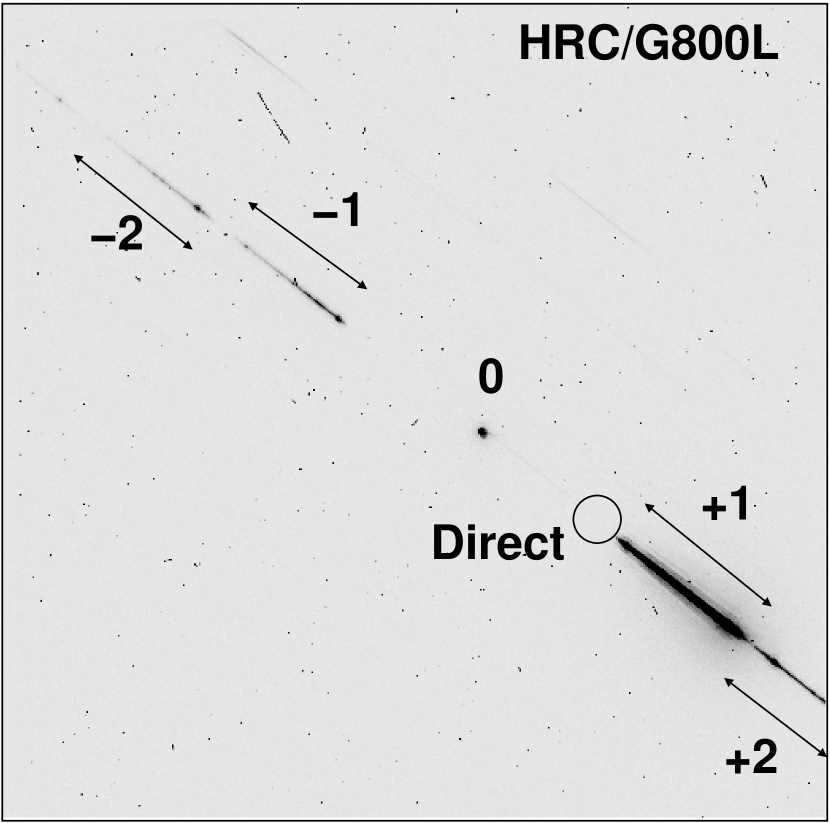
Figure 9: As in Figure 8, but for the HRC. The position of the object in the direct image is represented with a circle. The image size is 1024 $\times$ 1024 pixels.

The mean spectral tilt across the HRC field of view is -38^o.19 $\pm$ 0^o.12 from the image X axis (cf. Figure 9). The spectral tilt decreases from the top left to the bottom right corner by $\sim$ 0^o.05, and by $\sim$ 0^o.33 along the diagonal from the bottom left to the top right corner of the field of view (Pasquali et al. 2003b).

The Y-offset is on average -1.5 pixels with little field dependence, while the X-offset between the grism 0^th order and the object in the direct image is 145 pixels (as shown in Figure 9).

Both the grism 1^st and 2^nd orders are about 195 pixels along the spectral trace, while the -1^st and -2^nd orders are $\sim$ 183 and 174 pixels, respectively. As for the WFC/grism configuration, the sensitivity of the 2^nd order redward of 8000 Å is so low that the 2^nd order spectrum is not detected any longer and turns out to be as extended as the 1^st. The 0^th order is dispersed over 9 pixels along the spectral trace and its FWHM is 6 pixels.

8 The method for calibrating in wavelength

The wavelength calibration of the grism spectra of WR45 and WR96 relies on the set of template spectra taken for these two stars at medium resolution with the ESO NTT/EMMI spectrograph.

Two different approaches were adopted for determining the wavelength solutions. We first summarize the analysis of the SMOV and INTERIM data, which is described in more detail in Pasquali et al. (2003a). In this case, the WFC/HRC grism spectra were extracted with the ST-ECF package aXe (Pirzkal et al. 2001a, Pirzkal et al. 2003a,b), adopting an extraction aperture 2 pixels wide (to sample the peak of the instrument PSF) and the background was estimated 100 pixels away from the spectral trace. Since no wavelength solution had been defined at this stage, the wavelength scale of the extracted spectra was in units of pixels along the spectral trace, relative to the position of the object in the direct image. Seven emission lines can be identified in the extracted $\pm$1^st and 3^rd orders, while three to five lines are identified in the $\pm$2^nd and -3^rd orders. We measured for the WFC a mean line FWHM_WR of 3, 4 and 6 pixels in the $\pm$1^st, $\pm$2^nd and $\pm$3^rd orders, and for the HRC 4 and 6 pixels for the $\pm$1^st and 2^nd orders respectively.

The NTT template spectra were convolved with a gaussian function whose $\sigma$ was set to FWHM_WR/2.36 in order to mimic the ACS grism spectra. We reidentified the emission line in the new “degraded” templates, and measure their centroid wavelength via multi-gaussian fitting and deblending. At the same time and with the same procedure, the line centroids were measured in the WFC/HRC grism spectra in units of pixels. This method produced a table of line peak wavelengths and pixels for each grism order, which were then fitted to derive the wavelength solution of each spectral order. Clearly, the order of the fit depends on the number of identified lines available and on the S/N ratio in the extracted WFC/HRC grism spectra.

For the analysis of the INTERIM and Cycle 12 WFC observations of WR96 (Larsen & Walsh 2005) the grism spectra were again extracted with aXe as before, except that an extraction box width of 10 pixels was used. The wavelength solutions were then determined by fitting the NTT spectra directly to the ACS grism spectra. The AMOEBA routine (Press et al. 1992) was used to minimize the r.m.s. difference between the smoothed NTT spectra and the grism spectra as a function of the smoothing length and the wavelength solution coefficients. Since the ACS spectra were not flux calibrated at this stage, we also fitted for a wavelength-dependent sensitivity curve, approximated for this purpose as a 4th order polynomial. Figure 7 shows the smoothed NTT spectrum of WR96 and the ACS grism spectrum for the best-fitting wavelength solution. Clearly, the fit is not perfect, perhaps partly due to real temporal variations in the spectra of the WR star. Repeated iterations of the AMOEBA fits were made, each with slightly different initial guesses for the fit parameters to test the repeatability of the fits. Generally, the wavelength zero-points reproduced within a few Å and the dispersions to within 0.1 Å pixel^-1. All these procedures were applied to each grism order for each position across the field of view.

9 The in-orbit wavelength solutions of the WFC grism

An example of 2D grism images taken with the WFC and the HRC is shown for WR96 in Figures 8 and 9 respectively, where the different grism orders have been also identified. In these Figures we compare the location of the grism orders with the object position in the direct image. The WR45 spectra for the positive and negative orders taken at the center of Chip 1 are plotted in Figure 10, in units of counts vs wavelength in Å.

In the case of the WFC/grism observations, six orders (from the -3^rd to the +3^rd orders) were detected together with the 0^th order. Their wavelength solutions computed for the pointings across the WFC field of view are summarized in Tables 3 and 4. The blank entries indicate that the order was not detected because it fell outside the physical area of the chips. These wavelength solutions have been computed from the combined INTERIM and Cycle 12 calibration data (Larsen & Walsh 2005). They are reassuringly similar to those obtained from the SMOV/INTERIM data (that are omitted, for this reason, from this paper. For more details cf. Pasquali et al. 2003a). Indeed, the difference between the two calibrations is generally less than one pixel. Thus, users who have been using the older calibrations can consider their wavelength scales accurate to better than about 1 WFC pixel, but for future applications we recommend that the updated calibrations be used. These will be available via the ST-ECF web pages.

The wavelength solution obtained for the 1^st and 2^nd orders is a second order polynomial in the form of: $\lambda$ = $\lambda_{0}$ + $\Delta\lambda_{0}$X^′ + $\Delta\lambda_{1}$X^′2, where $\lambda_{0}$ is the wavelength zero point in Å, $\Delta\lambda_{0}$ the first term of the dispersion in Å/pix and $\Delta\lambda_{1}$ the second term of the dispersion in Å/pix². X^′ is the distance from the X coordinate of the object in the direct image along the spectral trace.

For the 1^st order, the first term of the dispersion $\Delta\lambda_{0}$ significantly varies across the field of view, with an amplitude of about 20$\%$ (of the value measured at the center of the field) from the the top, left corner to the bottom, right corner. Along this same direction, the wavelength zero point and the second term of the dispersion vary by $\sim$ 20 Å and a factor of $\sim$ 2 respectively.

In the case of the 2^nd order, $\Delta\lambda_{0}$ varies by about 10$\%$ of the dispersion measured at the center of the field, along the diagonal from the top, left corner to the bottom, right corner of the field of view. Along this same direction, the wavelength zero point increases by $\sim$ 220 Å.

The wavelength solutions of the positive 3^rd and all the negative orders are a first order polynomial in the form of: $\lambda$ = $\lambda_{0}$ + $\Delta\lambda_{0}$X^′. They exhibit the same field dependence as for the positive 1^st and 2^nd orders, with $\Delta\lambda_{0}$ varying by about 15$\%$ from the center to the bottom, right corner of the field of view.

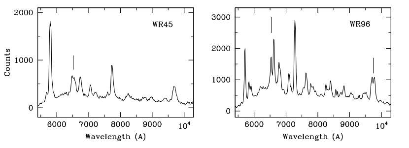
Figure 11: The third order spectra of WR45 and WR96. The split lines are indicated with a vertical line.

It is worth noticing here that the 3^rd orders are out of focus. Since the focal plane is tilted with respect to the optical axis the higher orders are more displaced from the optical axis. Consequently, a number of lines appear split when compared with the template spectra of WR45 and WR96 (cf. Figure 11, where the split lines are indicated with a vertical line).

10 The in-orbit wavelength solutions of the HRC grism

In the HRC grism data we detected six orders together with the 0^th order, from the -3^rd to the +3^rd order. Because of the position of WR45 across the field of view and the severe tilt of the spectra, the $\pm$3^rd orders are truncated and only a pair of emission lines can be identified. We thus do not provide any wavelength solution for these orders.

The $\pm$1^st and $\pm$2^nd order spectra acquired at the center of the field of view are plotted in Figure 12 in units of counts vs wavelength in Å. The wavelength solutions obtained across the HRC field of view are listed in Tables 5 and 6 (cf. Pasquali et al. 2003b).

The wavelength solution of the 1^st order is fitted with a second order polynomial as in the case of the WFC 1^st order. The dispersion is seen varying by 8$\%$ between the top, left corner to the bottom, right corner of the field of view. In this case, the field dependence follows the same diagonal as for the WFC, only in the opposite direction. The wavelength zero point also varies by 0.2$\%$ between these two edges of the field.

A first order polynomial traces the wavelength solution of the grism 2^nd order. The dispersion varies again by $\sim$ 8$\%$ from the top, left corner to the bottom, right corner of the field, and it is accompanied by a variation of 0.3$\%$ in the wavelength zero point.

The -1^st and -2^nd orders are detected only in two positions, at the center and the bottom, right corner of the field.

11 The grism flux calibration

The flux calibration of the ACS grism requires the correction for flat-field and for the total grism throughput, which takes into account the intrinsic grism response, the quantum efficiency of the CCD detectors and the throughput of the telescope and instrument optics.

In the case of slitless spectroscopy, the flat-field is field and wavelength dependent at the same time. Indeed, depending on the coordinates of a source in the direct image, the same pixel in the grism image is exposed to different wavelengths during different telescope pointings and grism acquisitions. A grism flat-field can be then constructed via interpolation of the flat-fields available for different imaging filters at any pixel position and wavelength, i.e. what is refereed to as a flat-field cube. For this purpose, we used a 3^rd order polynomial as a function of pixel coordinates and wavelength, which is directly used by the extraction package aXe (Pirzkal et al. 2003a,b). Technically, the correction for flat-field is applied following the wavelength calibration of a spectrum: only at this point, it is possible to extract a monodimensional flat-field from the flat-field cube in correspondence with the source position in the direct image and the wavelength range of the source spectrum.

Ideally, the grism flat-field cube should be constructed from the flat-fields of narrow-band filters, in order to better sample the wavelength space of the grism spectra and therefore to perform an accurate flux calibration. Practically, the available grism flat-field cubes (for the WFC and the HRC at http://www.stecf.org/instrument/acs) are based on in-orbit flat-fields for broad-band filters which describe the large scale variations in the CCD response up to $\lambda\sim$ 9000 Å.

In the case of the WFC, taking the broad-band filter flat-fields at face value generates a grism flat-field cube which produces flux discrepancies among the grism spectra of the standard star GD153 (the same occurs for G191B2B) observed at different positions across the field of view. These differences in flux possibly arise from a large-scale flat properties of the grism images that are different from those seen in direct images. In addition, since the imaging flat-fields are designed to give a flat image of the sky, their application to a grism image introduces a correction for the geometric distortions which is already been taking into account in the wavelength calibration of the extracted spectra. Consequently, the differences in flux among the standard star spectra taken in different positions were fitted with a 2D surface which was used to generate a corrected grism flat-field cube, able to produce spectra of the same star which agree within 1$\%$ between 6000 Å and 9000 Å and 2 - 3$\%$ at redder wavelengths, all across the field of view of the WFC (Pirzkal et al. 2003a,b, Walsh & Pirzkal 2005).

In the case of the HRC, the standard star GD153 was observed only in three positions out of the five which were adopted for the wavelength calibration. A simple grism flat-field cube, without any correction as applied to the WFC cube, generates spectra whose fluxes already agree within 2 $\%$, most likely because of the much lower degree of geometric distortions in the HRC with respect to the WFC (Pirzkal et al. 2003b).

The spectra extracted for GD153 and G191B2B, calibrated in wavelength and properly corrected for flat-field and CCD gain, were normalized by the exposure time, and divided by the STSDAS template spectrum calibrated in flux. The resulting sensitivity functions (in e^- pix^-1 Å per erg cm^-2 Å^-1) were averaged into a single grism response curve independent of the position across the chip and the standard deviation of the mean was assumed to be the error on the grism throughput. The errors in the absolute flux calibration are then 3$\%$ between 5000 Å and 9000 Å and 20$\%$ past 10000 Å. The mean WFC/HRC grism responses obtained for the 1^st order are plotted in Figure 13. They are delivered with the aXe package and can be found at http://www.stecf.org/software/aXe together with the grism higher order responses.

A secondary effect in the WFC/HRC grism spectra is fringing, due to the interference between the incident light and the light reflected at the interfaces between the thin layers of the CCDs. The modeling of fringes is possible once the layer composition of the CCD detector, the thickness and material of these layers are known. In the case of ACS, these parameters are not available (the WFC CCDs have proprietary construction), and are estimated by comparison of a fringe model with narrow-band filter flat-fields.

Walsh et al. (2003) have found that the peak-to-peak amplitude of the fringes in the HRC ($\simeq$ 27$\%$) is reproduced by assuming a CCD model with four layers: the Si top layer 12.5 - 16.0 $\mu$m thick, the second SiO₂ layer 0.26 $\mu$m in thickness, the third Si₃N₄ and the fourth Si layers with a 0.23 $\mu$m and 0.83 $\mu$m thickness respectively. Similarly, the WFC fringes are characterized by a peak-to-peak amplitude of $\simeq$ 24$\%$ which is reproduced by the same four layers CCD model adopted for the HRC, only with different thicknesses: 12.6 - 17.0 $\mu$m for the top layer, 1.14 $\mu$m, 0.90 $\mu$m and 3.08 $\mu$m for the second, third and fourth layer respectively.

The predictions of the above CCD models can be use to correct the narrow-band filter flat-fields for fringing: the net result is a decrease of the fringes peak-to-peak amplitude of about four.

Does fringing affect grism spectra? The incident light on the grism is convolved with the instrument PSF along both the dispersion and cross-dispersed axes. In the case of the WFC, the FWHM of the PSF is $\simeq$ 2.5 pixels, or 100 Å assuming $\Delta\lambda_{0}$ = 40 Å. The fringes period is $\sim$70 Å, therefore the PSF has the net effect of smoothing out the fringes envelope, by a factor of six as SLIM simulations show. Therefore, fringing in the WFC grism spectra is practically negligible. Since the grism dispersion is higher when coupled with the HRC ($\Delta\lambda_{0}$ $\simeq$ 24 Å) and the fringes period is 65 Å, some residual fringing may still be observed in HRC grism spectra (Walsh et al. 2003).

At the present time, a routine for the fringing correction is being planned for aXe.

12 From the calibrations to the users

The in-orbit calibrations of the ACS grism served the purpose to characterize its physical properties (i.e. spectral tilt) and the wavelength solution for each of its detected orders. Equally important, the calibrations were performed in selected positions across the WFC and HRC fields of view to verify the field dependence of the grism properties. The next step is therefore to be able to extract and calibrate a spectrum in wavelength and flux at any position in the field of view. This is achieved by interpolating each of the quantities derived in the previous sections across the chip as a function of the (X,Y) coordinates of the calibration stars, WR45 and WR96, in the direct image. Each interpolation describes the smooth spatial variation of the grism properties.

Specifically, the quantities that need to be interpolated are: the spectral tilt, the Y-offset and, for each order, the dispersion (the second term of the dispersion when available) and wavelength zero point. In the case of the WFC, the observed positions allowed us to parameterize the grism field dependence with second-order 2D polymonials, which, in the case of the grism 1^st order, are characterized by an error of 0^o.03 in the spectral tilt, 0.10 pixels in the Y-offset, 10 and 5 Å in the wavelength zero point in Chip 1 and 2, respectively, 0.6$\%$ and 0.4$\%$ in the first ($\Delta\lambda_{0}$) term of the dispersion in Chip 1 and 2, respectively. The second ($\Delta\lambda_{1}$) term is characterized by a r.m.s of 27$\%$ and 22$\%$ in Chip 1 and 2, respectively (Larsen & Walsh 2005). These interpolations were used to extract the spectra of the Planetary Nebula SMP-81, which in turn confirmed the consistency of the grism wavelength calibration.

Since only 5 positions were acquired across the HRC field of view, we interpolated the grism properties with a first-order 2D polynomial, which, for the 1^st order, has errors of 0^o.0005 in the spectral tilt, 0.4 pixels in the Y-offset, 4.8 Å (i.e. 0.2 pixels) in the wavelength zero point and 0.2$\%$ and 10$\%$ in the first ($\Delta\lambda_{0}$) and second ($\Delta\lambda_{1}$) terms of the dispersion (Pasquali et al. 2003b).

The coefficients of the 2D polynomials fitting the field dependence of the grism properties are stored in configuration files (one for each WFC chip and one for HRC) which are used by aXe and can be retrieved at http://www.stecf.org/software/aXe. The configuration files contain three other fundamental keywords: the name of the flat-field cube to be applied for the flat-field correction, the name of the sensitivity function for the flux calibration and the length of the orders in pixels.

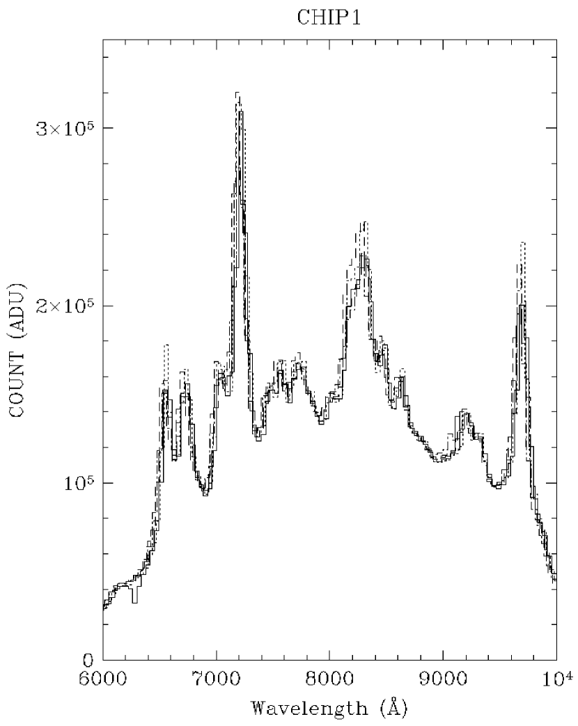
Figure 14: The spectra of WR96 extracted in 5 positions across Chip 1 of the Wide Field Channel.

To test the consistency of our interpolation, we re-extracted the spectra of WR45 and WR96 with aXe and the configuration files described above. Figure 14 shows the results for the different pointings across Chip 1 of the WFC. The spectra coincide within 0.4 [$\sim$ 16 Å, or 0.2 pixels ($\sim$ 5 Å) in the case of the HRC].

13 Concluding remarks

Observations with the ACS grism require science targets to be imaged through a filter (direct image) and the grism (grism image). The reason is that the target position in the direct image defines the zero point in the wavelength calibration and the flat-field correction for the flux calibration of a spectrum in the grism image.

Calibration data have shown that the object position in the direct image is independent of the filter used for imaging and is stable within 25 mas (0.5 pixels) when multiple acquisitions are performed within the same orbit. Direct images taken of the same target with the same POSTARG values during different orbits are instead stable within 100 mas (2 pixels). While a shift of $<$ 0.5 pixels (i.e. about 20 Å in the grism first order spectrum) is within the uncertainties of the wavelength calibration, an offset of 2 pixels introduces a systematic error of $\sim$ 80 Å in the wavelength calibration of the grism 1^st order. It is thus advisable to always acquire a direct image of the targeted field together with its grism images. In the case of multiple exposures of the same field with dither shifts, it suffices to have one direct image corresponding to one of the grism images and to use the 0^th orders to confirm the telescope shifts (e.g. this technique was applied by Pirzkal et al. 2004 to the GRAPES data).

Direct images can be combined to increase the S/N threshold for the detection of faint objects, but the positions of the objects measured in the final drizzled version have to be related to positions in the raw, geometrically distorted frame for a correct use of aXe (cf. Pirzkal et al. 2004). A spectroscopic drizzle task has been implemented in the latest version of aXe (aXe-1.4, Kümmel et al. 2004), which extracts 2D stamp images of a source spectrum appearing in multiple grism images, fully calibrated in wavelength and corrected for flat field. In the most general case, the source has been imaged in different positions across the field of view, therefore, because of the field dependence of the spectral dispersion, its spectra are characterized by different spectral dispersions. The aXe drizzle corrects the tilt of the individual spectral stamp image, so that its dispersion and the cross-dispersed axes are parallel to the x and y axes, respectively. It also makes the wavelength scale and the pixel scale in the cross-dispersed direction the same in all the spectral stamp images of the source. These drizzled stamp images are then coadded, and the final 1D spectrum of the source is extracted and flux calibrated, using a weighting scheme based on the S/N variations as provided by the drizzle weights (hence proportional to the different exposure times of the observations). Users can set the wavelength scale and the pixel scale in the cross-dispersed direction in the aXe configuration file; this option allows to enhance the resolution (spectral and angular) of the extracted spectra if the original data were taken with subpixel stepping.

The ACS slitless grism is equivalent to a ground-based multi-object spectrograph. The absence of a slit, though, affects the grism resolution, which the object size and inclination with respect to the dispersion axis can easily decrease (cf. Sect. 3). This effect can be modeled by, for example, deconvolving the spectrum by the spatial profile of the source, once the latter is known as a function of wavelength. In addition, the large extension of the grism orders may cause spectra of two adjacent objects to overlap. In its present form aXe provides a quantitative estimate of contamination but it does not correct for spectra contamination. Therefore it is suggested to acquire data using different telescope roll angles so to vary the direction of the dispersion axis and reduce the amount of spectra overlap. Also, orienting the telescope so that the dispersion axis is aligned with the object minor axis, certainly maximizes the spectral resolution achievable for that target. A final note has to be spent on the background level. Since each pixel of the spectrum sees the background emission integrated over the whole spectral range of the grism, the use of a high S/N background image, properly scaled to the exposure time of the data, will improve the S/N in the extracted spectra of faint sources.

As already mentioned before, ACS slitless grism spectroscopy has extensively been carried out by large programs such as APPLES (ACS Pure Parallel Ly$\alpha$ Emission Survey, PI Rhoads, ID 9482), GRAPES (Grism ACS Program for Extragalactic Science, PI Malhotra, ID 9793) and PEARS (Probing Evolution and Reionization Spectroscopically, PI Malhotra, ID 10530). GRAPES in particular has proved that the ACS grism can detect the continuum emission of sources as faint as z_AB = 27.2 mag and up to $z\sim$ 7 using 40 orbits (Pirzkal et al. 2004). This is the deepest slitless spectroscopy survey to date, even when compared with ground-based telescopes. It has allowed to characterize several types of galaxy population: Lyman break and Ly$\alpha$ galaxies at 4 $<z<$ 7 (Rhoads et al. 2005), old stellar populations at 0.5 $<z<$ 2.5 (Daddi et al. 2005, Pasquali et al. 2005), and emission line galaxies at $z<$ 1.5 (Pirzkal et al. 2005b), often at a luminosity level fainter than previously reached. The success of these surveys clearly indicate that the ACS grism spectroscopy provides important insights on galaxy evolution at high redshift.

Figure 1: The spectral resolution of the WFC and HRC grism as a function of the object size. The solid line represents 1^st order spectra and the dashed line corresponds to 2^nd order spectra. The object diameter along the dispersion axis is plotted in abscissa as a multiple of the PSF FWHM in arcsecs. The line FWHM is represented in the ordinate axis as a multiple of the mean FWHM in Å computed from the lines in the spectrum of a source 0^′′.05 in diameter.

Figure 4: The NTT/EMMI spectra of WR45 (top) and WR96 (bottom).

Figure 5: Observations of WR96. The object positions in the direct image used for programs 9568 (INTERIM) and 10058 (Cycle 12) are shown with triangles and boxes, respectively.

Figure 6: The map of the pointings (i.e. object positions in the direct image) used for WR45 and WR96 across the field of view of the HRC.

Figure 7: The smoothed NTT spectrum of WR96 and the ACS/WFC grism spectrum for the best fitting wavelength solution.

Figure 10: The spectra of the six grism orders detected in the WFC data and obtained for WR45.

Figure 12: The WR45 spectra of the four orders detected and calibrated in the HRC data.

Figure 13: The sensitivity functions of the grism 1^st order when coupled with the WFC and the HRC.

Table 1: Basic parameters of the selected WR stars, WR45 and WR96.

Star	Spectral type	RA(2000)	DEC(2000)	V	$v_{\infty}$ (km s-1)
WR45	WC6	11:38:05.2	-62:16:01	14.80	2100
WR96	WC9	17:36:24.2	-32:54:29	14.14	1100

Table 2: The exposure times adopted for each star and spectral element.

Target	F625W	F775W	G800L
WFC:
WR45	1 s	1 s	20 s
WR96		1 s	20 s
WR96		1 s	15 s
LMC-SMP-81		15 s	200 s
G191B2B		1 s	15 s
GD153		2 s	60 s
HRC:
WR45		3 s	60 s
GD153		6 s	180 s

Table 3: The wavelength solutions of the 1^st, 2^nd and 3^rd orders, determined for the different pointings across the field of view of the WFC.

Position	First order			Second order			Third order
	$\lambda_{0}$	$\Delta\lambda_{0}$	$\Delta\lambda_{1}$	$\lambda_{0}$	$\Delta\lambda_{0}$	$\Delta\lambda_{1}$	$\lambda_{0}$	$\Delta\lambda_{0}$
WFC/CHIP1
(29, 1883)	4762.17	35.50	0.00414	2546.53	16.91	0.00306	1529.99	12.46
(29, 1883)	4763.12	35.49	0.00432	2550.02	16.88	0.00314	1537.05	12.44
(54, 296)	4769.58	37.27	0.00480	2634.18	16.91	0.00549	1537.22	13.06
(1939, 1058)	4733.32	39.93	-0.00007	2628.73	17.82	0.00556	1541.92	13.64
(1940, 1057)	4738.62	39.98	-0.00025	2636.27	17.76	0.00570	1540.71	13.65
(3396, 1638)	4765.84	40.21	0.00542	2652.97	18.11	0.00657	1552.87	14.03
(3396, 1638)	4764.46	40.24	0.00519	2653.43	18.08	0.00666	1538.95	14.07
(3381, 269)	4776.26	41.87	0.00771	2633.99	19.22	0.00644	1543.18	14.71
(2950, 223)	4778.30	41.81	0.00414	2708.75	18.15	0.00865	1546.97	14.53
(3662, 1820)	4751.05	40.61	0.00373	2577.85	18.99	0.00437	-	-
(2959, 1778)	4769.01	39.67	0.00367	2629.52	18.08	0.00552	1565.00	13.75
(163, 1910)	4756.89	35.98	0.00279	2508.35	17.42	0.00202	1564.33	12.44
(1111, 1915)	4768.77	36.99	0.00420	2607.01	17.06	0.00446	1575.82	12.83
(1125, 337)	4776.17	38.97	0.00352	2657.27	17.41	0.00635	1553.18	13.55
(2044, 257)	4769.19	40.56	0.00302	2710.59	17.52	0.00817	1547.22	14.05
(2045, 1054)	4774.98	39.24	0.00451	2665.68	17.50	0.00664	1559.31	13.66
WFC/CHIP2
(3332, 1784)	4746.52	43.32	0.00334	2699.07	18.72	0.00917	1548.27	14.94
(3322, 400)	4777.15	44.73	0.00806	2728.65	19.34	0.01084	1536.41	15.71
(3322, 400)	4782.92	44.67	0.00852	2727.76	19.36	0.01081	1544.99	15.69
(303, 1779)	4761.05	38.56	0.00327	2609.03	17.63	0.00511	1389.09	13.77
(314, 380)	4782.26	39.77	0.00721	2614.51	18.40	0.00555	1532.86	14.04
(314, 380)	4772.47	39.86	0.00669	2665.29	17.79	0.00720	1553.76	13.98
(2023, 1934)	4774.60	40.78	0.00462	2701.40	17.79	0.00816	1551.22	14.20
(2024, 1934)	4775.98	40.94	0.00348	2698.68	17.85	0.00805	1563.61	14.18
(3642, 309)	4758.08	45.90	0.00491	2730.46	19.61	0.01124	1541.64	15.93
(2954, 253)	4774.10	44.81	0.00476	2764.58	18.74	0.01207	1555.78	15.54
(225, 289)	4775.20	39.98	0.00561	2607.48	18.45	0.00548	1529.12	14.04
(1151, 327)	4786.96	41.63	0.00497	2646.24	18.83	0.00664	1534.97	14.55
(2059, 268)	4788.72	43.10	0.00545	2672.69	19.25	0.00793	1559.76	15.02

Table 4: The wavelength solutions of the -1^st, -2^nd and -3^rd orders, determined for the different pointings across the field of view of the WFC.

Position	Negative First order		Negative Second order		Negative Third order
	$\lambda_{0}$	$\Delta\lambda_{0}$	$\lambda_{0}$	$\Delta\lambda_{0}$	$\lambda_{0}$	$\Delta\lambda_{0}$
WFC/CHIP1
(29, 1883)	-	-	-	-	-	-
(29, 1883)	-	-	-	-	-	-
(54, 296)	-	-	-	-	-	-
(1939, 1058)	-4965.81	-40.61	-2317.55	-19.66	-1472.93	-12.91
(1940, 1057)	-5045.09	-40.83	-2319.40	-19.65	-1472.69	-12.90
(3396, 1638)	-5069.28	-42.43	-2355.43	-20.47	-1531.79	-13.49
(3396, 1638)	-5081.47	-42.47	-2374.06	-20.52	-1565.35	-13.54
(3381, 269)	-5123.16	-44.59	-2340.16	-21.39	-1530.69	-14.13
(2950, 223)	-5115.70	-43.85	-2376.59	-21.14	-1485.96	-13.84
(3662, 1820)	-5094.49	-42.70	-2377.55	-20.61	-1490.10	-13.50
(2959, 1778)	-5077.32	-41.56	-2359.10	-20.06	-1554.45	-13.26
(163, 1910)	-	-	-	-	-	-
(1111, 1915)	-5046.21	-38.53	-2334.57	-18.56	-1287.35	-11.90
(1125, 337)	-5048.17	-40.47	-2348.77	-19.53	-1565.10	-12.91
(2044, 257)	-5110.14	-42.33	-2367.31	-20.38	-1494.76	-13.36
(2045, 1054)	-5091.67	-41.17	-2359.96	-19.84	-1494.91	-13.00
WFC/CHIP2
(3332, 1784)	-5094.14	-45.24	-2375.18	-21.84	-1623.83	-14.51
(3322, 400)	-5129.59	-47.57	-2377.74	-22.90	-1666.43	-15.31
(3322, 400)	-5096.84	-47.42	-2381.09	-22.91	-1621.90	-15.23
(303, 1779)	-	-	-	-	-	-
(314, 380)	-	-	-	-	-	-
(314, 380)	-	-	-	-	-	-
(2023, 1934)	-5059.91	-42.64	-2352.79	-20.57	-1460.89	-13.46
(2024, 1934)	-5069.51	-42.64	-2356.22	-20.57	-1478.50	-13.48
(3642, 309)	-5310.33	-49.11	-2381.69	-23.31	-1482.93	-15.25
(2954, 253)	-5111.24	-47.01	-2548.88	-23.09	-1456.04	-14.79
(225, 289)	-	-	-	-	-	-
(1151, 327)	-5056.06	-43.33	-2352.71	-20.91	-1522.75	-13.77
(2059, 268)	-5109.74	-45.28	-2369.10	-21.81	-1463.58	-14.24

Table 5: The wavelength solutions of the 1^st, 2^nd and 3^rd orders, determined for the different pointings across the field of view of the HRC.

Position	First order			Second order
	$\lambda_{0}$	$\Delta\lambda_{0}$	$\Delta\lambda_{1}$	$\lambda_{0}$	$\Delta\lambda_{0}$
(572, 574)	4755.91	23.86	0.0018	2475.29	12.00
(207, 944)	4749.06	24.59	0.0019	2471.58	12.35
(754, 391)	4759.68	23.51	0.0019	2480.18	11.82
(199, 391)	4756.92	23.87	0.0018	2476.84	11.99
(764, 949)	4753.80	24.19	0.0021	2471.41	12.19

Table 6: The wavelength solutions of the -1^st, -2^nd and -3^rd orders, determined for the different pointings across the field of view of the HRC.

Position	Negative first order		Negative second order
	$\lambda_{0}$	$\Delta\lambda_{0}$	$\lambda_{0}$	$\Delta\lambda_{0}$
(572, 574)	-5182.09	-26.75	-2762.80	-13.54
(207, 944)	-	-	-	-
(754, 391)	-5191.30	-26.40	-2732.50	-13.31
(199, 391)	-	-	-	-
(764, 949)	-	-	-	-

References

- (1) Acker, A., Ochsenbein, F., Stenholm, B. et al., 1992, Strasbourg-ESO Catalogue of Galactic Planetary Nebulae (ESO)
- (2) Blakeslee, J.P., Tsvetanov, Z.I., Riess, A.G. et al., 2003, ApJ, 589, 693
- (3) Ciardullo, R., Jacoby, G.H., Ford, H.C., Neill, J.D., 1989, ApJ, 339, 53
- (4) Daddi, E., Renzini, A., Pirzkal, N. et al., 2005, ApJ, 626, 680
- (5) de Mello, D.F., and Pasquali, A. 2001, A&A, 378, L10
- (6) Freudling, W., 1999, NICMOSlook User Manual 3.1
- (7) Freudling, W., Pirzkal, N., 1997, NICMOSlook User Manual 1.1
- (8) Fruchter, A.S., Hook, R.N., 1998, astro-ph/9808087
- (9) Hack, W. 1992, FOC ISR 065
- (10) Hack, W. 1996, FOC ISR 092
- (11) Hook, R.N., Fruchter, A.S., 2000, in Astronomical Data Analysis Software and Systems IX, ASP Conference Proceedings, 216, 521
- (12) Horne, K., and MacKenty, J. 1991, WFPC1 ISR 008
- (13) Jacoby, G.H., Ciardullo, R., 1999, ApJ, 515, 169
- (14) Jakobsen, P., Albrecht, R., Barbieri, C. et al. 1993, ApJ, 417, 528
- (15) Jansen, R.A., and Jakobsen, P. 2001, A&A, 370, 1056
- (16) Kümmel, M., Walsh, J.R., Larsen, S., Hook, R., 2004, ST-ECF Newsletter 36, 10
- (17) Larsen, S., Walsh, J.R., 2005, Updated Wavelength Calibration for the WFC/G800L Grism, ST-ECF ISR ACS, in preparation
- (18) Magee, D., Bouwens, R., Illingworth, G. et al., 2002, IAU Circ 7908
- (19) Malhotra, S., Rhoads, J.E., Pirzkal, N. et al., 2005, ApJ, 626, 666
- (20) McCarthy, D.W., Campins, H., Kern, S. et al., 1998, AAS, DPS, 30, 1114
- (21) McCarthy, P.J., Yan, L., Freudling, W. et al., 1999, ApJ, 520, 548
- (22) Mutchler, M., Cox, C., 2001, STScI ISR ACS 2001-07
- (23) Noll, K. et al., 2004, NICMOS Instrument Handbook, Version 7.0, (Baltimore: STScI)
- (24) Paresce, F., and Greenfield P. 1989, FOC ISR 038
- (25) Pasquali, A., Ferreras, I., Panagia, N. et al., 2005b, ApJ, accepted
- (26) Pasquali, A., Larsen, S., Ferreras, I. et al., 2005a, AJ, 129, 148
- (27) Pasquali, A., Pirzkal, N., Walsh, J.R. et al., 2001a, ST-ECF ISR ACS 2001-02
- (28) Pasquali, A., Pirzkal, N., Walsh, J.R., 2001b, ST-ECF ISR ACS 2001-04
- (29) Pasquali, A., Pirzkal, N., Walsh, J.R., 2003a, ST-ECF ISR ACS 2003-01
- (30) Pasquali, A., Pirzkal, N., Walsh, J.R., 2003b, ST-ECF ISR ACS 2003-02
- (31) Pirzkal, N., Pasquali, A., 2001, ST-ECF Newsletter 28, p. 3
- (32) Pirzkal, N., Pasquali, A., Demleitner, M., 2001a, ST-ECF Newsletter 29, p. 5
- (33) Pirzkal, N., Sahu, K.C., Burgasser, A. et al., 2005a, ApJ, 622, 319
- (34) Pirzkal, N., Pasquali, A., Walsh, J.R., et al., 2001b, ST-ECF ISR ACS 2001-01
- (35) Pirzkal, N., Pasquali, A., Walsh, J.R., 2003a, in 2002 HST Calibration Workshop, STScI 2002, eds. S. Arribas, A. Koekemoer & B. Whitmore, p. 74
- (36) Pirzkal, N., Pasquali, A., Walsh, J.R., 2003b, ST-ECF ISR ACS 2003-04
- (37) Pirzkal, N., Xu, C., Ferreras, I. et al., 2005b, ApJ, accepted (astro-ph/0509551)
- (38) Pirzkal, N., Xu, C., Malhotra, S. et al., 2004, ApJS, 154, 501
- (39) Plait, P. 1998a, AAS, 192, 6706
- (40) Plait, P. 1998b, AAS, 193, 9802
- (41) Press, W. H., Teukolsky, S. A., Vetterling, W. T., & Flannery, B. P., 1992, Numerical Recipes in C/Fortran, Cambridge University Press
- (42) Rhoads, J.E., Panagia, N., Windhorst, R.A. et al. 2005, ApJ, 621, 582
- (43) Riess, A.G., Strolger, L.-G., Tonry, J. et al., 2004, ApJ, 600, L163
- (44) Teplitz, H.I., Collins, N.R., Gardner, J.P., Rhoads, J.E., 2001, AJ, 122, 1023
- (45) Teplitz, H.I., Collins, N.R., Gardner, J.P. et al., 2003 ApJS, 146, 209
- (46) Tsvetanov, Z., Blakeslee, J., Ford, H. et al., 2002, IAU Circ. 7912
- (47) van der Hucht, K.A., 2001, The VIIth catalogue of galactic Wolf-Rayet stars, New AR, 45, 135
- (48) Walsh, J.R., Freudling, W., Pirzkal, N., Pasquali, A., 2003, ST-ECF ISR ACS 2003-03
- (49) Walsh, J.R., Pirzkal, N., 2005, ST-ECF ISR ACS 2005-02
- (50) Windhorst, R., Bernstein, R.A., Collins, N. et al., 2000, AAS, 197, 12301
- (51) Xu, C., Rhoads, J.E., Malhotra, S. et al., 2005, ApJ submitted
- (52) Young, P.R., and Dupree, A.K. 2002, ApJ, 565, 598