Search for massive protostar candidates in the southern hemisphere: II. Dust continuum emission

In an ongoing effort to identify and study high-mass protostellar candidates we have observed in various tracers a sample of 235 sources selected from the IRAS Point Source Catalog, mostly with $\delta<-30\degr$, with the SEST antenna at millimeter wavelengths. The sample contains 142 Low sources and 93 High, which are believed to be in different evolutionary stages. Both sub-samples have been studied in detail by comparing their physical properties and morphologies. Massive dust clumps have been detected in all but 8 regions, with usually more than one clump per region. The dust emission shows a variety of complex morphologies, sometimes with multiple clumps forming filaments or clusters. The mean clump has a linear size of $\sim 0.5$ pc, a mass of $\sim 320\leavevmode\nobreak\ M_{\odot}$ for a dust temperature $T_{\rm d}=30$ K, an H₂ density of $9.5\times 10^{5}$ cm^-3, and a surface density of 0.4 g cm^-2. The median values are 0.4 pc, $102\leavevmode\nobreak\ M_{\odot}$, $4\times 10^{4}$ cm^-3, and 0.14 g cm^-2, respectively. The mean value of the luminosity-to-mass ratio, $L/M\simeq 99\leavevmode\nobreak\ L_{\odot}/M_{\odot}$, suggests that the sources are in a young, pre-ultracompact Hii  phase. We have compared the millimeter continuum maps with images of the mid-IR MSX emission, and have discovered 95 massive millimeter clumps non-MSX emitters, either diffuse or point-like, that are potential prestellar or precluster cores. The physical properties of these clumps are similar to those of the others, apart from the mass that is $\sim 3$ times lower than for clumps with MSX counterpart. Such a difference could be due to the potential prestellar clumps having a lower dust temperature. The mass spectrum of the clumps with masses above $M\sim 100\leavevmode\nobreak\ M_{\odot}$ is best fitted with a power-law $dN/dM\propto M^{-\alpha}$ with $\alpha=2.1$, consistent with the Salpeter (salpeter55 (1955)) stellar IMF, with $\alpha=2.35$. On the other hand, the mass function of clumps with masses $10\leavevmode\nobreak\ M_{\odot}\lesssim M\lesssim 120\leavevmode\nobreak\ M_{\odot}$ is better fitted with a power law of slope $\alpha=1.5$, more consistent with the mass function of molecular clouds derived from gas observations.

1 Introduction

Massive stars ($M\geq 8\leavevmode\nobreak\ M_{\odot}$) play a crucial role in the appearance and evolution of galaxies. They are responsible for the production of heavy elements and influence the interstellar medium through energetic winds and supernovae. Despite their importance, the understanding of massive star formation has remained significantly behind that of their lower-mass counterparts, for which much observational and theoretical work has already been done. This situation has changed in recent years, when the formation of high-mass stars has been gaining increasing interest, with the attention gradually shifting from the study of clouds associated with ultracompact UC Hii regions, to those where only luminous IRAS sources without radio continuum emission were detected. This is equivalent to approaching the earliest stages of high-mass star formation, when most of the luminosity of the newly formed (proto)star is derived from the release of gravitational energy.

Palla et al. (palla91 (1991)) have used the IRAS Point Source Catalog (IRAS-PSC) to select plausible candidates of massive (proto)stars with $\delta\geq-30\degr$. The basic criteria used by these authors to select the targets are based on the IRAS colours and the lack of association with Hii regions: the former constraint is derived from the study of Richards et al. (richards87 (1987)), who used IRAS colours to identify compact molecular clouds; the latter is aimed at biasing the sample towards high-mass Young Stellar Objects (YSOs) in a very early phase of their evolution, when an Hii region has not yet developed. The resulting sample was split into two sub-samples, this time using the IRAS colour selection criteria of Wood & Churchwell (wood89 (1989)) for identifying UC Hii regions: $[25-12]\geq 0.57$ and $[60-12]\geq 1.30$. The two sub-samples of compact molecular clouds satisfying and non-satisfying the Wood & Churchwell criteria have been called High and Low, respectively. The selected sources also verify that there are no upper limits for their fluxes at 25, 60, and 100 $\mu$m, and that $F_{60\mu{\rm m}}\geq 100$ Jy. Palla et al. (palla91 (1991)) have searched for H₂O maser emission associated with the sources and found a lower association rate for the Low sources that has been interpreted as an indication that the Low sources are in an earlier evolutionary phase than the High sources. Both sub-samples have been systematically observed in different continuum and molecular line tracers, from centimeter to near-infrared wavelengths (Molinari et al. moli96 (1996), 1998a , 1998b , moli00 (2000), moli02 (2002); Brand et al. brand01 (2001); Zhang et al. zhang01 (2001), zhang05 (2005)). The scope was to derive the physical properties of the two groups and confirm that they are in different evolutionary stages. In particular, the Low sub-sample would contain a fraction of young sources that are not yet zero-age main sequence (ZAMS) massive stars. The main findings of this study have been thoroughly discussed by Brand et al. (brand01 (2001)) and can be summarized as follow:

• High and Low sources have luminosities typical of high-mass YSOs ($L>10^{3}L_{\odot}$);

• the percentage of Low sources not associated with UC Hii regions is higher (76%; see Molinari et al. 1998a ) than that of High sources (57%);

• a large fraction of Low sources have dust temperatures of $\sim 30$ K (Molinari et al. moli00 (2000)) much lower than those measured towards “hot cores” ($\gtrsim 100$ K), and are hence most likely high-mass objects too young to have yet developed an UC Hii region.

In order to extend our systematic search for massive protostellar candidates to the entire sky, we have selected new targets in the southern hemisphere, namely High and Low sources with $\delta<-30\degr$. This is the second of a series of papers aimed to conduct in the southern hemisphere the same kind of investigation carried out for sources with $\delta\geq-30\degr$. In the first paper (Fontani et al. fontani05 (2005)) we have discussed the results of the molecular line survey towards the Low sources with $\delta<-30\degr$. The main results of that study are that there is a tight association of the sources with dense gas, and that the physical properties of the Low sources, such as linewidths, and distribution of the NRAO VLA Sky Survey NVSS-to-IRAS flux ratio, are comparable to those found by Sridharan et al. (srid02 (2002)) for a sample of High-like sources when the luminosity of the sources is $L<10^{5}L_{\odot}$. The mass-luminosity ratios are also similar to those found by Sridharan et al. (srid02 (2002)) but lower than the ratio found for a sample of UC Hii regions, supporting the idea that our Low sources, as well as those High-like of Sridharan et al. (srid02 (2002)), are younger than UC Hii regions. In the present paper we discuss the main findings of the millimeter continuum survey carried out towards a sample of High and Low sources with $\delta<-30\degr$, plus a few additional sources with $-30\degr<\delta<40\degr$. In particular we study the morphology of the dust emission and derive the physical properties of the sources, and compare them with those reported by other surveys in the literature. In addition, we also compare the properties of both High and Low sub-samples, as well as those of millimeter sources associated with mid-infrared sources from the Midcourse Space Experiment (MSX) Point Source Catalog and those that are not. Finally, we present a study on the mass spectrum of the observed sources.

2 Sample

The first step in extending the search for massive YSOs towards the southern hemisphere was to select a sample of possible candidates from the IRAS-PSC following the Palla et al. (palla91 (1991)) criteria. Taking into account the interest of studying the earliest stages of high-mass star formation, we first selected a sample of Low sources with $\delta<-30\degr$, which was observed in C¹⁷O and/or CS and the results are presented in the first paper by Fontani et al. (fontani05 (2005)). Out of the 131 sources of this sample, 125 were then observed in the continuum at millimeter wavelengths (the results of that survey are presented in this paper). In order to conduct a comparative study of their properties with those of possibly more evolved sources, we also observed in the continuum a comparable sample of High sources with $\delta<-30\degr$, which had been previously detected in CS by Bronfman et al. (bronfman96 (1996)). In addition we also observed a number of Low and High sources with $\delta>-30\degr$. The resulting sample observed in the millimeter continuum contains a total of 235 sources: 142 of them Low and 93 High. Table 1 shows the position, distance, and luminosity of the sources in the sample. As already mentioned, almost all (89%) the sources in our sample have $\delta<-30\degr$, whereas the Palla et al. (palla91 (1991)) sample contained only objects with $\delta\geq-30\degr$. Therefore, one may reasonably expect that our sample contains a higher contamination by Hii or UC Hii regions than that of Palla et al. (palla91 (1991)), because radio continuum surveys of Hii regions with $\delta<-30\degr$ are less numerous than and not as complete as those with $\delta\geq-30\degr$.

All the High sources in the sample have been previously detected in CS by Bronfman et al. (bronfman96 (1996)), and those with $\delta>-30\degr$, with the exception of IRAS 18198$-$1429, also in NH₃ by Molinari et al. (moli96 (1996)). The Low sources with $\delta<-30\degr$, with the exception of IRAS 15579$-$5347, have been observed in CS by Fontani et al. (fontani05 (2005)), and some of them have also been observed in C¹⁷O, and those with $\delta>-30\degr$ in NH₃ by Molinari et al. (moli96 (1996)). Fifteen of the Low sources with $\delta<-30\degr$ were not detected either in C¹⁷O or CS (Fontani et al. fontani05 (2005)).

3 Observations

The 1.2-mm continuum observations were carried out with the 37-channel bolometer array SIMBA (SEST Imaging Bolometer Array) at the SEST (Swedish-ESO Submillimetre Telescope), on July 16–20, 2002 and July 9–13, 2003.

Maps of $900\arcsec\times 400\arcsec$ (azimuth $\times$ elevation) around each IRAS source in Table 1 were obtained, with a scan rate of $80\arcsec/{\rm s}$, and a separation of $8^{\prime\prime}$ in elevation between scans. Bigger maps were also obtained by using a mosaicing technique towards sources 16153$-$5016, 17225$-$3426, and 18014$-$2428 (here and in the following we will refer to the sources without mentioning “IRAS” in the name). For the region surrounding source 16428$-$4109, the center of the observations was shifted $\sim 4\aas@@fstack{\prime}7$ northeast from the nominal IRAS point source position: after taking a first map centered at the IRAS position, no millimeter emission was detected at the source nominal position but there clearly was emission at the edge of the map, so we decided to shift the center towards the northeast. We have checked the HIgh RESolution (HIRES) IRAS images and have found that there is an infrared source at the nominal IRAS point source position, which indicates that the position given in the IRAS-PSC is correct. In our study we have considered as associated with the IRAS source all the millimeter clumps located at $<90^{\prime\prime}$ from the nominal IRAS point source position. Therefore, the clumps detected towards 16428$-$4109 are not associated with the IRAS source. The total integration time per map was about 15 minutes, and the typical noise level in the maps is 25–40 mJy beam^-1. Atmospheric opacity was determined from skydips, which were taken every 2 hours; values at zenith ranged between 0.21 and 0.50 (during the 2002 observations) and 0.13 and 0.30 (in 2003). The data were calibrated using observations of Uranus, made once or twice per day; the conversion factor ranged between 58 and 75 mJy/count in 2002, and between 50 and 69 in 2003. The calibration uncertainty is about 15%. The pointing of the SEST was determined to be accurate within a few arcsec by observing the strong continuum sources $\eta$ Carinae or Centaurus A every 2 hours. The HPBW is $\sim 24^{\prime\prime}$.

All data were reduced with the program MOPSI, written by R. Zylka (IRAM, Grenoble), according to the instructions given in the SIMBA Observers Handbook (2003). See Chini et al. (chini03 (2003)) for a detailed description of the data reduction method.

4 Results

4.1 Kinematic distances

Table 1 lists the kinematic distances, $d$, to the IRAS sources. The distances have been estimated, using the rotation curve of Brand & Blitz (brand93 (1993)), from the CS line velocity given by Bronfman et al. (bronfman96 (1996)) for all the High sources, from the CS line velocity given by Fontani et al. (fontani05 (2005)) for those Low with $\delta<-30\degr$, and from the NH₃ line velocity given by Molinari et al. (moli96 (1996)) for the Low sources with $\delta>-30\degr$. This method is valid for galactocentric distances between 2 and 25 kpc. For sources inside the solar circle, there are two solutions for the kinematic distance, near and far. In some cases this ambiguity can be solved, for example, when the height of the source from the galactic plane is more than 200 pc (i.e. roughly twice the scale height of the molecular disk) at the far distance, or when the near distance is too small for a massive star forming region. This is the case for sources 14394$-$6004 and 17040$-$3959, for which $d_{\rm near}$ is $<100$ pc, and therefore the far distance was adopted. There are many sources for which it was not possible to solve the distance ambiguity: for these in Table 1 we report both distance estimates. Note that in the following to derive the physical parameters of the sources and in case of unsolved distance ambiguity, the near distance is adopted. The distances to the IRAS sources are between 130 pc and 27.1 kpc, with an average value of $\sim 4.5$ kpc, and a median value of $\sim 3.8$ kpc.

We have not been able to derive an estimate of the distance for sources 08488$-$4457, 10088$-$5730, 10156$-$5804, 10575$-$5844, 11431$-$6516, 11476$-$6435, 12434$-$6355, 13078$-$6247, 13558$-$6159, 14198$-$6115, 14412$-$5948, 15506$-$5325, 15579$-$5347, 16204$-$4943, 16581$-$4212, 17140$-$3747, 17230$-$3531, 17231$-$3520, 17242$-$3513, 17352$-$3153, 17410$-$3019, 17425$-$3017. There are three possible reasons for that: no estimate of the systemic velocity of the region was available; the corresponding distances estimates are outside the galactocentric interval 2–25 kpc; the height from the galactic plane is too large ($>200$ pc) for near and far distances.

Most of the regions observed contain more than one millimeter clump (see Section 4.3), and it is likely that all of them belong to the same star forming region as the IRAS source. Therefore, when deriving their physical parameters, we have made the assumption that all the clumps are located at the same kinematic distance as the one estimated for the IRAS source.

4.2 Luminosities

The bolometric luminosities in Table 1 were calculated by integrating the IRAS flux densities. The contribution from longer wavelengths was taken into account by extrapolating according to a black-body function that peaks at 100 $\mu$m and has the same flux density as the source at this wavelength. The distribution of luminosities is shown in Fig. 1. The average luminosity is $\sim 6.7\times 10^{4}L_{\odot}$ and the median is $\sim 1.6\times 10^{4}L_{\odot}$. These luminosities are $\sim 3.5$ times lower than the average and median values derived by Faúndez et al. (faundez04 (2004)) for their sample of southern sources. This could be due to the fact that their sample has been selected from the survey of Bronfman et al. (bronfman96 (1996)), which contains high-mass very YSOs but it is also contaminated by more evolved sources such as Hii regions (or equivalently more massive stars), which are expected to be brighter at far-infrared wavelengths.

Figure 1: Histogram of the luminosity distribution calculated from the IRAS flux densities of the sources.

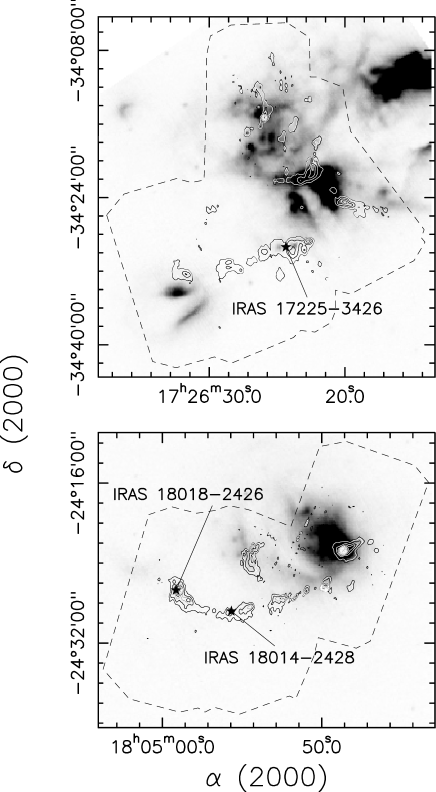
Figure 3: Overlay of the 1.2 mm continuum emission (contours) obtained with SIMBA at the SEST antenna, on the MSX emission at 21 $\mu$m (Band E) (image) towards the sources IRAS 17225$-$3426 (upper panel) and IRAS 18014$-$2428 (bottom panel). The contour levels range from 0.11 (3$\sigma$) to 1.67 Jy beam^-1 in steps of 0.22 Jy beam^-1 (upper panel) and from 0.09 (3$\sigma$) to 3.20 Jy beam^-1 in steps of 0.17 Jy beam^-1 (bottom panel). The star marks the position of the IRAS sources. The coordinates are in J2000 epoch. In the bottom panel, the two IRAS sources correspond to Mol 36 (IRAS 18014$-$2428) and Mol 37 (IRAS 18018$-$2426) from Molinari et al. (moli96 (1996)). The dashed polygon shows the limits of the area mapped with SIMBA.

4.3 Identification of the clumps

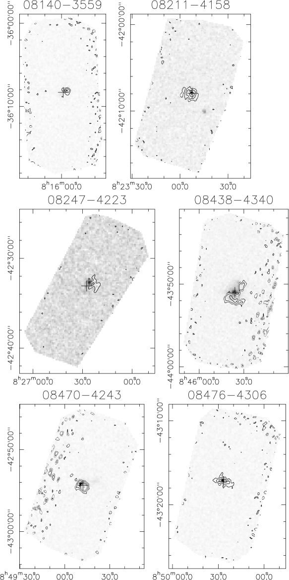
Figure 2: Overlay of the 1.2 mm continuum emission (contours) obtained with SIMBA at the SEST antenna, on the MSX emission at 21 $\mu$m (Band E) (image) towards the sources of our survey. The contour levels are 3$\sigma$, 6$\sigma$, and from 6$\sigma$ to the maximum integrated emission in steps of 6$\sigma$, where $\sigma$ is the rms noise of each map. The equatorial coordinates are in J2000 epoch. The noisy edges of the SIMBA map are visible. The black cross marks the nominal IRAS point source position. For IRAS 16428$-$4109, the imaged field is offset by $4\aas@@fstack{\prime}7$ from the nominal IRAS point source position. For IRAS 18014$-$2428/18018$-$2426, the two IRAS sources correspond to Mol 36 (IRAS 18014$-$2428; black cross) and Mol 37 (IRAS 18018$-$2426; black triangle) from Molinari et al. (moli96 (1996)).

Massive dust clumps have been detected in all but 7 regions, 10102$-$5706, 11476$-$6435, 14198$-$6115, 15571$-$5218, 16403$-$4614, 16417$-$4445, and 18024$-$2231, of our sample. As already mentioned in Section 3, for 16428$-$4109, the clumps are displaced by $\sim 4\aas@@fstack{\prime}7$ from the position of the IRAS source. The millimeter maps of our survey are shown in Fig. 2. Figure 3 shows the two largest areas mapped in our survey, that is, the mosaiced maps towards sources 17225$-$3426 and 18014$-$2428. As can be seen in the maps, there is usually more than one clump per region. In some cases the large number of clumps and the extended emission detected in the region make it very difficult to separate them from each other by eye. Therefore, in order to identify the millimeter clumps and their properties adopting a more objective criterion, we have used a two-dimensional variation of the clump-finding algorithm Clumpfind developed by Williams et al. (williams94 (1994)). The three-dimensional version of the algorithm was originally designed to be applied to spectral line datacubes, and the two-dimensional version is a simple modification of it. The algorithm works by effectively contouring the data at a multiple of the rms noise of the map, then searching for peaks of emission to locate the clumps, and finally following the clump profile down to lower intensities. The contouring levels have to be chosen by hand, which means that the clump-finding procedure is not completely automated, and therefore one can introduce biases into the results. Clumpfind does not a priori require any particular shape of the clump profile, as some other clumps finding algorithms do, and one of its disadvantages is that it misses low-mass clumps that lie below the lowest contour. This could flatten the low-mass end of the mass spectrum of the regions. In our case, we set the lowest contour level to 3$\sigma$, and then increased the contouring by steps of 3$\sigma$.

The clump-finding procedure calculates the peak position, the full width at half maximum (FWHM) not corrected for beam size for the x-axis, ${\rm FWHM_{x}}$, and for the y-axis, ${\rm FWHM_{y}}$, and the total flux density integrated within the clump boundary, that is within the lowest contour level. Table 2 gives the offset positions in arcsec with respect to the nominal IRAS point source position for each clump, the angular diameter, which has been calculated as the deconvolved geometric mean of ${\rm FWHM_{x}}$ and ${\rm FWHM_{y}}$, the linear diameter, the total flux density, the mass, and the density. The last column indicates whether the clump is associated with MSX emission, either point-like or diffuse, or not. Figures 4a and 4b show the histograms with the kinematic distance of the clumps and the number of clumps per region. The mean and median values of the distance of the clumps are 3.9 kpc and 3.4 kpc, respectively, while those of the number of sources per region are 2.8 and 2.0, respectively. Note that the values of the mean and median distance are slightly lower when taking into account all the clumps in the regions instead of taking only into account the central IRAS source (see Section 4.1). The maximum number of clumps have been detected in the large mosaiced maps around sources 17225$-$3426 and 18014$-$2428, for which we have found 27 and 22 clumps, respectively (see Fig. 3).

Figure 4: Histograms of some parameters of the clumps detected in the continuum emission at 1.2 mm: (a) kinematic distance, (b) number of clumps per map, (c) radius of the clumps, (d) mass of the clumps, (e) H₂ volume density, and (f) H₂ surface density. Note that in the regions for which mosaiced observations were carried out, we have included all the clumps in the field when computing the histograms, and not only the sources in a field $900^{\prime\prime}\times 400^{\prime\prime}$, like for the other regions.

4.4 Morphologies of the clumps

The 1.2 mm maps in Fig. 2 show that the dust emission towards massive star forming regions presents a variety of complex morphologies. The emission, which usually peaks at or near the IRAS position, is very often associated with multiple compact embedded objects and extended emission. Sometimes the emission is very centrally peaked, with a single massive clump associated with the IRAS source, e.g. 12063$-$6259, 15454$-$5335, and 18144$-$1723, sometimes with more than one massive clump clustered towards the central position, e.g. 12127$-$6244, 13333$-$6234, and 17149$-$3916, or with smaller and fainter clumps clustered or located nearby, e.g. 15015$-$5720, 15519$-$5430, 17082$-$4114, and 17118$-$3090. Sometimes the emission shows multiple clumps located throughout the field, which can be separated from each other, e.g. 16085$-$5138, 16093$-$5128, 16153$-$5016, and 17242$-$3513, or linked in a chain of clumps and elongated structures, e.g. 10184$-$5748, 13039$-$6108, 14000$-$6104, and 16164$-$4929, suggesting star formation in a sheet or a filament (e.g. Larson larson85 (1985)). Particularly nice examples of this latter phenomenon are seen in the mosaiced maps of 17225$-$3426 and 18014$-$2428 (Fig. 3) that show strings of emission clumps and elongated and clustered structures. Sometimes the emission towards the IRAS position is very faint (e.g. 08488$-$4457, 10277$-$5730, and 15464$-$5445), or no millimeter emission is detected at all. In particular, the number of IRAS sources not detected at 1.2 mm is 12, taking into account 10545$-$6244, 16153$-$5016, 16428$-$4109, and 17156$-$3607 as well, for which although there are millimeter clumps detected in the region, none of them is associated (i.e. within $90^{\prime\prime}$) with the IRAS source. All of them are ${\it Low}$ sources. As can be seen in Table 3 of Fontani et al. (fontani05 (2005)), 5 of them, 16403$-$4614, 16417$-$4445, 16153$-$5016, 16428$-$4109, and 17156$-$3607 have been detected in CS and C¹⁷O, 3 of them, 10102$-$5706, 15571$-$5218, and 10545$-$6244 have been detected in CS but not in C¹⁷O, and 3 of them, 11476$-$6435, 14198$-$6115, 14412$-$5948, have not been detected in CS but not been observed in C¹⁷O. Finally, one of the sources, 18024$-$2231, has been detected in NH₃ by Molinari et al. (moli96 (1996)). On the other hand, there are 6 Low sources, 08488$-$4457, 10088$-$5730, 12434$-$6355, 15506$-$5325, 16204$-$4943, and 16581$-$4212, that have been detected in the millimeter continuum, although the emission is faint, but not in CS (Fontani et al. fontani05 (2005)), and one source, 15579$-$5347, that has not been observed in CS and has been clearly detected in the continuum.

4.5 Linear Diameters

The deconvolved linear diameters of the clumps have been computed from their angular diameters. As mentioned in Sect. 4.3, both linear and angular diameters are listed in Table 2. The mean value is $0.5$ pc for those sources that have been resolved, which is in agreement with the average value of 0.6 pc found by Williams et al. (williams04 (2004)) for the sources of the Sridharan/Beuther sample (Sridharan et al. srid02 (2002); Beuther et al. beuther02 (2002)), and quite smaller than the value of 0.8 pc found by Faúndez et al. (faundez04 (2004)), or 1 pc found by Hill et al. (hill05 (2005)) for their samples of southern sources, although it is not clear whether the sizes given by these authors have been deconvolved or not. The median value for the clumps in our sample is 0.4 pc. Figure 4c shows the histogram of the radius of the clumps.

We have searched for possible asymmetries in the clumps by calculating ${\rm FWHM_{x}}/{\rm FWHM_{y}}$. The mean and median values obtained, 1.04 and 0.96, respectively, indicate that the clumps are quite symmetric.

4.6 Masses and densities

The masses of the clumps given in Table 2 have been estimated assuming that the dust emission is optically thin, by using

$$M_{\rm clump}=\frac{g\,S_{\nu}\,d^{2}}{\kappa_{\nu}\,B_{\nu}(T_{\rm d})},$$ (1)

where ${S_{\nu}}$ is the flux density, $d$ is the distance to the source, ${\kappa_{\nu}}$ is the dust mass opacity coefficient, $g$ is the gas-to-dust ratio, and $B_{\nu}(T_{\rm d})$ is the Planck function for a blackbody of dust temperature $T_{\rm d}$, all measured at $\nu=250$ GHz. We adopted $\kappa_{250}$ = 1 cm² g^-1 (Ossenkopf & Henning ossenkopf94 (1994)), $g=100$, and $T_{\rm d}=30$ K for all the sources. Estimates of $T_{\rm d}$ have been obtained by fitting grey-bodies to the spectral energy distribution (SED) of those IRAS sources that have only one millimeter clump associated with them. As already done by Fontani et al. (fontani05 (2005)) for the Low sources in our sample, we have neglected the IRAS fluxes at 12 and 25 $\mu$m in the fit. The reason for this choice is that two components are known to be present in the SEDs of luminous YSOs (see Sridharan et al. srid02 (2002) and Beuther et al. beuther02 (2002)): one associated with compact, hot gas and dominating the 12 and 25 $\mu$m fluxes; the other due to parsec-scale, colder material, contributing to the 60 and 100 $\mu$m emission. The latter component is the one of interest to us, because we want to estimate the temperature of the parcsec-scale clumps mapped at 1.2 mm. Adopting a dust absorption coefficient proportional to $\nu^{2}$, we have found best fits with mean temperatures of 28 K for both Low and High sources. Therefore, taking into account that for most of our clumps there are not enough measurements at different wavelengths to properly fit their SEDs (for some of them the 1.2 mm is the only one available), we have decided to adopt $T_{\rm d}=30$ K for all the clumps. A similar value, $T_{\rm d}=32\pm 5$ K, has been found by Molinari et al. (moli00 (2000)) for a sample of 30 luminous Low sources in the northern hemisphere. Furthermore, Faúndez et al. (faundez04 (2004)), who have fitted the SED of a sample of southern hemisphere sources similar to the High sources in our sample with grey-bodies with two components, have found an average value $T_{\rm d}\simeq 32$ K for the colder component.

Figure 5: (a) Histograms of the distribution of the luminosity-to-mass ($L/M$) ratio for all the sources, where $M$ is the sum of the masses of clumps located $<90^{\prime\prime}$ from the nominal IRAS point source position. (b) Same as above, for the Low (solid line) and the High sources (dashed line).

Figure 4d shows the histogram of the distribution of masses of the clumps. The mean value of the clump mass is 320 $M_{\odot}$, although the median mass is much lower, $102\leavevmode\nobreak\ M_{\odot}$. These values are in agreement with those of 330 $M_{\odot}$ and 143 $M_{\odot}$, respectively, found by Williams et al. (williams04 (2004)) for the 68 high-mass protostellar candidates of the Sridharan/Beuther sample (Sridharan et al. srid02 (2002); Beuther et al. beuther02 (2002)) assuming the near kinematic distance. Williams et al. (williams04 (2004)) have derived their clump masses using the dust opacity coefficients of Ossenkopf & Henning (ossenkopf94 (1994)), and $T_{\rm d}$ ranging from 30 to 60 K. Note that the average value of $5.0\times 10^{3}\leavevmode\nobreak\ M_{\odot}$ given by Faúndez et al. (faundez04 (2004)) refers to the total mass in each region; i.e., the sum of the masses of all the clumps in that region. If we take into account all the clumps in each region the average mass is 955 $M_{\odot}$, which is still five times lower than the one derived by Faúndez et al. (faundez04 (2004)). This could be due to the fact that their sample contains more massive stars, as already suggested by the bolometric luminosities of their targeted sources (see Section 4.2). Hill et al. (hill05 (2005)) in their recent survey of massive star-forming regions harbouring methanol masers and/or radio continuum sources have reported an average mass for their sample of $1.5\times 10^{3}\leavevmode\nobreak\ M_{\odot}$, and a median value of $1.0\times 10^{3}\leavevmode\nobreak\ M_{\odot}$, for a dust temperature of 20 K. The average mass would be $\sim 0.9\times 10^{3}\leavevmode\nobreak\ M_{\odot}$ and the median $\sim 0.6\times 10^{3}\leavevmode\nobreak\ M_{\odot}$, for a dust temperature of 30 K, which is the one that we have used for our estimates. Such values are still much higher than the ones of our sample. This, again, could indicate that the YSOs in their sample are intrinsically more massive. Unfortunately these authors do not report the bolometric luminosity of the sources, and we cannot corroborate this hypothesis.

Figures 4e and 4f show the histograms of the H₂ volume density and surface density of the clumps. These have been derived assuming that the clumps have spherical symmetry and a mean molecular weight of $\mu=2.29m_{\rm H}$. The average values are $9.5\times 10^{5}$ cm^-3 and 0.4 g cm^-2, respectively, and the median values are $4\times 10^{4}$ cm^-3 and 0.14 g cm^-2, respectively.

Figure 6: Histogram of the luminosity distribution calculated from the IRAS flux densities, for the Low (solid line) and the High sources (dashed line).

5 Discussion

5.1 The Luminosity-Mass relation

An important parameter for establishing the age of a core is the luminosity-to-mass ratio, $L/M$. This ratio is expected to increase with time as more and more gas is converted into stars during the star formation process and the embedded cluster becomes more luminous. Figures 5a and 5b show respectively the $L/M$ ratio for all the sources in our sample, and for the Low and the High sub-samples separately. The luminosity has been derived from the IRAS flux densities (see Sect. 4.2), and the mass is the sum of the masses of the clumps located $<90^{\prime\prime}$ from the nominal IRAS point source position (see Table 1), as we have considered only these clumps as associated with the IRAS source. The mean value of the distribution is $99\leavevmode\nobreak\ L_{\odot}/M_{\odot}$ for all the sources, and $98\leavevmode\nobreak\ L_{\odot}/M_{\odot}$ and $101\leavevmode\nobreak\ L_{\odot}/M_{\odot}$ for the Low and the High sub-samples, respectively. These values are in agreement with the value of $100\leavevmode\nobreak\ L_{\odot}/M_{\odot}$ found by Sridharan et al. (srid02 (2002)) for the sources of the Sridharan/Beuther sample, when rescaled to the Ossenkopf & Henning (ossenkopf94 (1994)) opacity of 1 cm² g^-1 used by us to derive the masses. Sridharan et al. (srid02 (2002)) report an average value of $0.05\leavevmode\nobreak\ M_{\odot}/L_{\odot}$, based on the masses derived by Beuther et al. beuther02 (2002)), which were estimated using the opacity of Hildebrand (hildebrand83 (1983)). This opacity is $\sim 2.5$ times smaller than the Ossenkopf & Henning opacity at 250 GHz. However, note that the masses estimated by Beuther et al. beuther02 (2002)), as recently reported by these authors, are wrong by a factor of 2 (see Beuther et al. beuther05 (2005)); that is, they should be a factor of 2 lower. Therefore, the average value of the $M/L$ ratio for their sample is actually $0.025\leavevmode\nobreak\ M_{\odot}/L_{\odot}$, or $40\leavevmode\nobreak\ L_{\odot}/M_{\odot}$, which rescaled to the opacity of Ossenkopf & Henning is $100\leavevmode\nobreak\ L_{\odot}/M_{\odot}$. These values are slightly higher than the average value of $71\leavevmode\nobreak\ L_{\odot}/M_{\odot}$ reported by Faúndez et al. (faundez04 (2004)). However, as already mentioned, these authors have used the sum of the masses of all the clumps in each region in their calculations. If we sum the mass of all the clumps in the regions, the average value that we obtain is $77\leavevmode\nobreak\ L_{\odot}/M_{\odot}$ , a value similar to the one reported by those authors.

No significant difference is seen between the mean value of $L/M$ for the Low and the High sources. The same conclusion has been found by Fontani et al. (fontani05 (2005)) when comparing the Low sources of our sample with the High sources of the sample of Sridharan/Beuther (Sridharan et al. srid02 (2002); Beuther et al. beuther02 (2002)). These latter authors have compared the $L/M$ values of the sources in their sample with those of known UC Hii regions with the same masses (Hunter hunter97 (1997), Hunter at al. hunter00 (2000)) and have found a $L/M$ ratio 5 times higher for the latter. Note that all these masses have been wrongly calculated by these authors with a factor 2 higher (see Beuther et al. beuther05 (2005)). However, this error do not change the conclusions derived from their comparison, as both are affected by the same factor. Mueller et al. (mueller02 (2002)) and Faúndez et al. (faundez04 (2004)) have found a similar result, although the difference between cores associated with UC Hii regions and those not associated reported by these authors is not statistically significant. Sridharan et al. (srid02 (2002)) have suggested that the difference in $L/M$ ratio occurs because the sources in their sample are in a younger pre-UC Hii phase, and that $L/M$ increases as the cores evolve and develop UC Hii regions. Taking into account that the sources in our sample have $L/M$ ratios similar to those of the Sridharan/Beuther sample (see Sect. 4.6), we conclude that they too are younger than UC Hii  regions.

Figure 7: Histograms of (a) kinematic distance, (b) number of clumps per map, (c) radius of the clumps, (d) mass of the clumps, (e) H₂ volume density, and (f) H₂ surface density, for the Low (solid line) and the High sources (dashed line). Note that in the regions for which mosaiced observations were carried out, we have included all the clumps in the field when computing the histograms, and not only the sources in a field $900^{\prime\prime}\times 400^{\prime\prime}$, like for the other regions.

5.2 Low versus High

One of the goals of this work is to carry out a comparative study of two sub-samples of massive YSOs, Low and High believed to be in different evolutionary stages. To do this one should check whether the two groups have different physical properties that could confirm a different evolutionary phase. Figure 6 shows the histogram of the luminosity distribution for both sub-samples, and Fig. 7 shows comparative histograms of some other physical properties, such as the number of clumps in each region, the size of the clumps, their mass, H₂ volume density, and surface density. As can be seen in these figures, both sub-samples Low and High are quite similar and do not show significant differences. This is the same conclusion reached by Fontani et al. (fontani05 (2005)) when comparing the properties (linewidth, luminosity, temperature, NVSS-to-IRAS flux ratio) of the Low sources in our sample with the High sources of the Sridharan/Beuther sample with luminosity $L<10^{5}L_{\odot}$.

Analyzing the properties in more detail, one can see that the luminosity distribution of the High sub-sample (Fig. 6) shows more sources at higher luminosities; the mean value for the High sub-sample, $1.3\times 10^{5}L_{\odot}$, is a factor of 5 higher than that for the Low sub-sample, $2.5\times 10^{4}L_{\odot}$. The median value, which is $2.6\times 10^{4}L_{\odot}$ for the High and $1.3\times 10^{4}L_{\odot}$ for the Low, is only a factor of 2 different. The mean number of clumps per region is similar for both sub-samples, 2.9 for the Low and 2.7 for the High, while the median number is 2.0 for both sub-samples. The maximum number of clumps per region are 27 and 22 and correspond to the mosaics around the Low sources 17225$-$3426 and 18014$-$2428, respectively. If one does not take into account these two regions, the maximum number of clumps per region are comparable, with 12 clumps for the Low source 17141$-$3606, and 10 for the High source 16085$-$5138. The morphologies of the clumps are quite similar in both sub-samples (see Fig. 2). Not surprisingly, the sources with fainter millimeter emission or no emission at all towards the IRAS position, which are mostly Low sources, have no C¹⁷O or CS detected (Fontani et al. fontani05 (2005)).

Some differences are evident in the linear size and the mass of the clumps, which have mean and median values of 0.46 pc and 0.38 pc, and $163\leavevmode\nobreak\ M_{\odot}$ and $64\leavevmode\nobreak\ M_{\odot}$ for the Low clumps, and 0.67 pc and 0.56 pc, and $561\leavevmode\nobreak\ M_{\odot}$ and $164\leavevmode\nobreak\ M_{\odot}$ for the High ones. Brand et al. (brand01 (2001)) have found an opposite result for the linear diameters of sources with $\delta\geq-30$, as they have found that clumps around Low sources are $\sim 3$ times larger than those around High clumps. However, those linear diameters have been obtained from molecular line observations instead of from the dust continuum emission.

As explained in Sect. 4.6, we have derived a temperature of $\sim$30 K for all the clumps, with no significant difference between Low and High sources. We have estimated the masses of the clumps adopting this value. However, our temperature estimates are based on a very limited number of measurements, so that we cannot rule out the possibility that High sources are hotter than Low ones. As a matter of fact, while Faúndez et al. (faundez04 (2004)) have found a temperature (32 K) similar to ours for their sample of High-like sources, Sridharan et al. (srid02 (2002)) determined a higher value (50 K) for a similar sample. If one adopts 50 K also for our High sources, the mass estimates obtained by us should be multiplied by 0.55 and the mean value of the mass of the clumps would be $309\leavevmode\nobreak\ M_{\odot}$, which is still a factor $\sim 2$ higher than the mean value of the Low sources. Therefore, the difference in mass of the clumps seems to be real. Regarding the other physical properties, the H₂ volume density, and the surface density of the clumps, the average and median values are $1.4\times 10^{6}$ cm^-3 and $4.1\times 10^{4}$ cm^-3, and 0.45 g cm^-2 and 0.13 g cm^-2 for the Low sources, and $2.6\times 10^{5}$ cm^-3 and $3.9\times 10^{4}$ cm^-3, and 0.29 g cm^-2 and 0.16 g cm^-2 for the High ones.

We have searched for possible asymmetries in the Low and High clumps by calculating ${\rm FWHM_{x}}/{\rm FWHM_{y}}$, and we have found similar values for both sub-samples. The mean and median values are 1.04 and 0.95, respectively, for the Low clumps, and 1.03 and 0.97 for the High ones. Such values indicate that the clumps of both sub-samples are quite symmetric.

The two sub-samples seem to be in the same evolutionary stage, as suggested by the $L/M$ ratio (see Sect. 5.1). Therefore, in conclusion, there is no significant difference in the physical parameters derived from the present millimeter continuum observations of the Low and High sub-samples with $\delta<-30\degr$. Both seem to be hosting high-mass (proto)stars with similar physical properties ($M$, $n_{\rm H_{2}}$, radius, $L/M$) and evolutionary stage. However, in order to reasonably compare the results of our southern study of Low and High sources with those obtained in previous northern hemisphere ($\delta\geq-30\degr$) studies (Palla et al. palla91 (1991); Molinari et al. moli96 (1996), 1998a , moli00 (2000); Brand et al. brand01 (2001)) which found differences between both sub-samples, more observations at different wavelengths of line and continuum emission are still needed in the southern hemisphere. In particular, it would be very important to properly estimate the temperature of the sources, either through some molecular line observations, or though more infrared and (sub)millimeter observations to better constrain their SEDs. Such temperature estimates could tell us whether the Low sources are colder, and therefore younger, than the High sources, as observed in the northern hemisphere.

Figure 8: Histogram of the 1.2 mm to 21 $\mu$m integrated flux density ratio for clumps associated with point-like MSX emission (solid line). The dashed line indicates the median value of $S_{\rm mm}/(1.5$ Jy), where $S_{\rm mm}$ is the 1.2 mm integrated flux density and 1.5 Jy is the MSX detection limit at 21 $\mu$m, for those clumps that are not associated with MSX emission. Note that due to the fact that these clumps have not been detected at 21 $\mu$m, the median value of the ratio $S_{\rm mm}/(1.5$ Jy) is a lower limit.

5.3 MSX versus non MSX

Figure 9: Histograms of (a) radius of the clumps, (b) mass of the clumps, (c) H₂ volume density, and (d) H₂ surface density, for clumps associated with MSX emission, either point-like or diffuse (solid line), and those that are not (dashed line). Note that in the regions for which mosaic observations were carried out, we have included all the clumps in the field when computing the histograms, and not only the sources in a field $900^{\prime\prime}\times 400^{\prime\prime}$, like for the other regions.

As seen in the previous sections, the IRAS sources in our sample are usually associated with massive clumps likely hosting high-mass (proto)stars. In an attempt to approach even closer to the earliest stages of high-mass star formation, it would be of great interest to identify a core prior to the star formation process; namely a prestellar or, better called, precluster core. Such a precluster core is expected to have density and size similar to those with embedded high-mass protostars, but lower luminosity and temperature. The bulk of its luminosity is expected to be emitted at millimeter and submillimeter wavelengths, with faint or no mid-IR or far-IR emission. One may reasonably expect that such cores capable of forming massive stars but in a stage prior to the onset of star formation are located close to massive luminous cores containing already formed high-mass (proto)stars. The millimeter continuum maps have shown that there is usually more than one millimeter clump in the region surrounding the IRAS source, and that not all of them are associated with it; that is, they are located at $>90^{\prime\prime}$ from the nominal IRAS point source position. Therefore, we have searched for precluster cores in the surroundings of the candidate massive (proto)stars by cross-correlating our sample with the MSX Point Source Catalog, since the diameters of the clumps are comparable to the spatial resolution of $18\aas@@fstack{\prime\prime}3$ of the mid-IR MSX observations. The cross-correlation has been done searching for mid-IR point sources in a radius of $40^{\prime\prime}$ around each millimeter clump, in any of the four bands (8 $\mu$m, 12 $\mu$m, 14 $\mu$m, or 21 $\mu$m) in the MSX-PSC version 6.0. In case that more than one millimeter clump was found at $\leq 40^{\prime\prime}$ from the same MSX point source, we have arbitrarily chosen the nearest clump as the associated one. We have also compared by eye the millimeter continuum maps with images of the MSX emission (see Fig. 2), which has allowed us to identify millimeter sources associated with mid-IR extended or diffuse emission. In the last column of Table 2 it is indicated whether the clumps are associated with point-like or diffuse MSX emission, or have no MSX emission at all. The positions in the MSX-PSC are accurate to an rms of $4^{\prime\prime}$–$5^{\prime\prime}$, and the calibration uncertainties are well within 13% (Egan et al. egan98 (1998)).

As a result of this study we have discovered 95 massive millimeter clumps not associated with mid-IR emission, meaning no mid-IR point source at any of the four bands, nor diffuse emission, that are potential precluster clumps (see Table 2). However, this number could be a lower limit because the excess of mid-IR emission in the observed regions produces, in some cases, confusion. Therefore, the association of some millimeter clumps with diffuse MSX emission may not be real. In addition, there are 35 clumps in the MSX-PSC detected only at 8 $\mu$m, whose emission could be due to contamination by Polycyclic Aromatic Hydrocarbons (PAHs) and not due to an embedded source. Until now only a very limited number of such candidates have been found in the northern (Molinari et al. 1998b ; Beuther et al. beuther02 (2002); Sridharan et al. srid02 (2002)), and southern hemisphere (Garay et al. garay04 (2004); Hill et al. hill05 (2005)). Note that in some cases, such as for example source 17221$-$3619, there are MSX sources located at the edge of the millimeter cores, which might be either reflection nebulae or sources belonging to the same star-forming region but in an older evolutionary stage: in fact, more evolved, and therefore hotter sources, are stronger emitters at mid-IR wavelengths. Seventy out of the 95 clumps without MSX emission are clumps in maps around Low sources, which is the 16% of the Low clumps, while 20 (10%) are clumps in maps around High sources. Therefore, the Low sub-sample contains in percentage more potential precluster clumps than the High sub-sample.

Figure 10: Left top panel: The mass spectrum of the 1.2 mm clumps detected at a distance $<6$ kpc. The solid line represents the Salpeter IMF, $dN/dM\propto M^{-2.35}$; the dotted line is a $-2.1$ power law, obtained from the least square fit to the data, and the dashed line is a $-1.7$ power law. The vertical dot-dashed line indicates the completeness limit at 6 kpc. Right top panel: The normalized cumulative mass distribution of clumps with masses above the completeness limit at 6 kpc. The solid, and dashed lines are the same as in the left panel, and the dotted line is a $-1.9$ power law, obtained from the least square fit to the data. Left bottom panel: Same as above for clumps detected at a distance $<2$ kpc. The vertical dot-dashed line indicates the completeness limit at 2 kpc. Right bottom panel: Same as above for clumps with masses above the completeness limit at 2 kpc.

Figure 8 shows the histogram of the 1.2 mm to 21 $\mu$m integrated flux density ratio for the clumps associated with point-like MSX emission, where the flux density at 21 $\mu$m has been taken from the MSX-PSC. The dashed line indicates the median value of $S_{\rm mm}/(1.5$ Jy), where $S_{\rm mm}$ is the 1.2 mm integrated flux density and 1.5 Jy is the typical MSX detection limit at 21 $\mu$m, for those clumps that are not associated with MSX emission. Note that because these clumps have not been detected at 21 $\mu$m, the detection limit flux of 1.5 Jy is an upper limit for their emission at 21 $\mu$m, and therefore, the median value of the ratio $S_{\rm mm}/(1.5$ Jy) is a lower limit. As can be seen in Fig. 8, there are relatively strong millimeter clumps that have no MSX counterpart, which indicates that they are not associated with mid-IR emission. Therefore, some of the 95 millimeter clumps without MSX counterpart could be in fact precluster clumps, where luminous stars have not yet formed.

Figure 9 shows the comparative histograms of some physical properties, such as the radius, mass, H₂ volume density, and surface density of the clumps associated with MSX emission, either point-like or diffuse, and those not. As can be seen in the distributions, the physical properties of the two sub-samples are similar. Due to the fact that the scale of the distributions is logarithmic, the properties would have to be very different in order to be clearly visible in the histograms. The main difference is the mass of the clumps, which for non-MSX emitters is clearly lower, with a mean value of $96\leavevmode\nobreak\ M_{\odot}$ and a median of $33\leavevmode\nobreak\ M_{\odot}$ compared with the mean and median values of $336\leavevmode\nobreak\ M_{\odot}$ and $106\leavevmode\nobreak\ M_{\odot}$, respectively, of the clumps with MSX counterparts. However, the dust temperatures of the clumps without mid-IR emission could be significantly lower than that of the clumps with embedded massive (proto)stars, which is $T_{\rm d}\sim 30$ K. In fact, Garay et al. (garay04 (2004)) have found $T_{\rm d}<17$ K for those clumps not associated with MSX emission in their sample. Assuming a dust temperature of 15 K, the masses of the clumps should be corrected by a factor $\sim 2.5$, and therefore, the masses of both MSX and non-MSX emitters would be more comparable. Regarding the other properties, the mean values for the size, H₂ volume density, and surface density are 0.3 pc, $4.7\times 10^{5}$ cm^-3, and 0.2 g cm^-2 for the clumps without MSX counterpart (the densities maybe also scaled by a factor $\sim 2.5$ like the mass, in case $T_{\rm d}=15$ K), and 0.5 pc, $9.6\times 10^{5}$ cm^-3, and 0.4 g cm^-2 for the clumps associated with mid-IR emission. The median values are 0.3 pc, $4.0\times 10^{4}$ cm^-3, and 0.11 g cm^-2 for the clumps without MSX counterpart, and 0.4 pc, $3.6\times 10^{4}$ cm^-3, and 0.14 g cm^-2 for those with MSX counterpart.

In order to assess whether the clumps without MSX emission are in an earlier evolutionary phase than the other ones, it would be necessary to map the cores in different molecular tracers to better derive their physical properties, and in particular their temperature, which should be lower for precluster cores.

5.4 The Mass Spectrum of the clumps

Table 3: Power law indices of the mass spectrum of the clumps, $dN/dM\propto M^{-\alpha}$, for different mass ranges. The mass of the clumps has been derived either from the dust continuum or from gas emission. The arrows indicate the whole mass range for which the fit to the mass spectrum has been done.

	Mass Range $(M_{\odot})$
	1.7–25	10–35	35–100	100–$10^{3}$	$10^{3}$–$10^{4}$
Dust emission
Tothill et al. (tothill02 (2002))	—	1.7	—	—	—
Beuther & Schilke (beuther04 (2004))	2.5	—	—	—	—
Williams et al. (williams04 (2004))	—	1.14		2.32
This Paper	—	1.5–1.9		2.1
Reid & Wilson (reid05 (2005))	—	0.9		2.0
Gas emission
Kramer et al. (kramer98 (1998))	—	1.6–1.7	1.6–1.8	1.7–1.8	1.7–1.8

Figure 10 shows the histogram of the mass spectrum of the 1.2 mm clumps detected at a distance $d<6$ kpc (top panels), and $d<2$ kpc (bottom panels). The completeness limit, which has been estimated by calculating the mass of a $5\sigma$ detection at the upper distance limit and is shown as a vertical dot-dashed line in the left panels, is $\sim 92\leavevmode\nobreak\ M_{\odot}$ at 6 kpc, and $\sim 10\leavevmode\nobreak\ M_{\odot}$ at 2 kpc. The right panels show the normalized cumulative mass distribution of clumps with masses above the completeness limit. The number of clumps above the completeness limit is 249 for $d<6$ kpc, and 79 for $d<2$ kpc. If the clump mass distribution can be represented by a power law of the type $dN/dM\propto M^{-\alpha}$, then the histogram of the mass spectrum can be fitted with a straight line of slope $-\alpha$. The solid line in the figures corresponds to $\alpha=2.35$, i.e., the Salpeter (salpeter55 (1955)) IMF; the dashed line to $\alpha=1.7$, corresponding to the mass function of molecular clouds derived from gas, mainly CO, observations (e.g. Kramer et al. kramer98 (1998)); and the dotted line corresponds to the slope computed from a least squares fit to our data. This value is $\alpha=2.10\pm 0.02$, with a fit correlation coefficient of 0.991, for the mass range $92\leavevmode\nobreak\ M_{\odot}\lesssim M\lesssim 4100\leavevmode\nobreak\ M_{\odot}$ ($d<6$ kpc), and $\alpha=1.90\pm 0.04$, with a fit correlation coefficient of 0.977, for the mass range $10\leavevmode\nobreak\ M_{\odot}\lesssim M\lesssim 387\leavevmode\nobreak\ M_{\odot}$ ($d<2$ kpc). However, if ones does not take into account the last noisy point in the mass spectrum ($M=387\leavevmode\nobreak\ M_{\odot}$) when computing the least squares fit, and fits the clumps detected at $d<2$ kpc with masses $10\leavevmode\nobreak\ M_{\odot}\lesssim M\lesssim 120\leavevmode\nobreak\ M_{\odot}$, the slope of the fitted mass spectrum is much flatter, $\alpha=1.50$, with a fit correlation coefficient of 0.999. Note that the errors reported for the slope values are those given by the fit, but do not represent the true uncertainties in the values of $\alpha$, which depend also on other factors such as the binning used to determine the mass spectrum.

As can be seen from Fig. 10, which shows the mass spectrum and the best-fit power law for two different mass ranges, the mass spectrum, for masses above the completeness limit, cannot be fitted by a single power law for the whole mass range; that is, for $10\leavevmode\nobreak\ M_{\odot}\lesssim M\lesssim 4100\leavevmode\nobreak\ M_{\odot}$. The clump mass spectrum is slightly steeper for the high-mass end ($M\gtrsim 100\leavevmode\nobreak\ M_{\odot}$), and it flattens for lower masses ($M\lesssim 100\leavevmode\nobreak\ M_{\odot}$): for clumps detected at $d<6$ kpc with masses above the completeness limit of $92\leavevmode\nobreak\ M_{\odot}$ (top left panel), the spectrum is well fitted with $\alpha=2.1$, consistent with a Salpeter-like power law; on the other hand, for clumps detected at $d<2$ kpc, with masses $10\leavevmode\nobreak\ M_{\odot}\lesssim M\lesssim 120\leavevmode\nobreak\ M_{\odot}$, the mass spectrum is better fitted with $\alpha=1.5$ or, if one takes also into account a clump with a mass $M\lesssim 387\leavevmode\nobreak\ M_{\odot}$, with $\alpha=1.9$, more consistent with the mass function of molecular gas clouds (e.g. Kramer et al. kramer98 (1998)).

Such a change in the slope of the mass spectrum has been previously detected in other dust emission single-dish surveys of massive very YSOs (see Table 3). Williams et al. (williams04 (2004)) have fitted the mass spectrum of their high-mass sample with a very flat slope, $\alpha=1.14$ for $M<100\leavevmode\nobreak\ M_{\odot}$, and with $\alpha=2.32$ for $M>100\leavevmode\nobreak\ M_{\odot}$. Reid & Wilson (reid05 (2005)) have fitted the submillimeter clump mass function in NGC 7538 with $\alpha=0.9\pm 0.1$ for the mass range $15\leavevmode\nobreak\ M_{\odot}\lesssim M\lesssim 100\leavevmode\nobreak\ M_{\odot}$, and with $\alpha=2.0\pm 0.3$ for the mass range $100\leavevmode\nobreak\ M_{\odot}\lesssim M\lesssim 2700\leavevmode\nobreak\ M_{\odot}$. In both cases, the breakpoint in the slope of the mass spectrum is well above the completeness limit of their samples, which suggests that the change in slope is real and not an observational effect. A power-law with $\alpha=1.7$ has been fitted by Tothill et al. (tothill02 (2002)) to the dust condensations with masses in the range $10\leavevmode\nobreak\ M_{\odot}\lesssim M\lesssim 35\leavevmode\nobreak\ M_{\odot}$ in the Lagoon Nebula, which is the same region that we have mapped in our mosaic around 18014$-$2428 (Fig. 3). Assuming that the break in the mass spectrum for massive dust clumps is real and not an artifact of the observations due to incompleteness, its shape is certainly interesting.

For $M\gtrsim 100\leavevmode\nobreak\ M_{\odot}$, the slope of the mass spectrum of the dust clumps is $\alpha=2.0$–2.32 (see Table 3). Such massive clumps are associated with pre- and protoclusters, so that the mass spectrum plotted in Fig. 10 could correspond to the pre- and protocluster mass distribution. Interestingly, a slope of 2–2.32 is similar to the clump mass distribution in low-mass star-forming regions, which for masses $0.5\leavevmode\nobreak\ M_{\odot}\lesssim M\lesssim 10\leavevmode\nobreak\ M_{\odot}$ mimics the stellar IMF (e.g. Testi & Sargent testi98 (1998); Motte et al. motte98 (1998); Johnstone et al. johnstone00 (2000), johnstone01 (2001)). The similarity between our result and those obtained in low-mass star-forming regions seems to suggest that the fragmentation of massive clumps may determine the IMF and the masses of the final stars. In other words, the processes that determine the clump mass spectrum might be self-similar across a broad range of clump and parent cloud masses. Reid & Wilson (reid05 (2005)), based on theories of molecular cloud evolution (e.g. Gammie et al. gammie03 (2003); Tilley & Pudritz tilley04 (2004)), suggest that turbulent fragmentation might be the dominant process that determines the shape of the clump mass spectrum.

For lower masses ($10\leavevmode\nobreak\ M_{\odot}\lesssim M\lesssim 100\leavevmode\nobreak\ M_{\odot}$) the slope of the mass spectrum is shallower and consistent with the one found for clumps of similar masses observed in molecular lines ($\alpha\sim 1.7$; Kramer et al. kramer98 (1998)). This is also shallower than the spectrum of lower mass ($M\lesssim 10\leavevmode\nobreak\ M_{\odot}$) pre- and protostellar dust clumps. However, such a comparison may be not appropriate because of the different tracer used in the line and continuum surveys, as line observations are more sensitive to low-density material than continuum imaging. Moreover, for our clumps the slope of the mass spectrum in the interval $10\leavevmode\nobreak\ M_{\odot}\lesssim M\lesssim 100\leavevmode\nobreak\ M_{\odot}$ is quite uncertain, because the mass range is relatively small and close to the completeness limit. Finally, the limited angular resolution of the single-dish observations of massive star-forming regions might be insufficient to resolve the clumps into the cores associated with individual (proto)stars. This makes it hazardous to compare the results with those of interferometric observations or with those of low-mass star-forming regions, which have a much higher angular resolution. In fact, Beuther & Schilke (beuther04 (2004)) resolved 12 clumps, with masses $1.7\leavevmode\nobreak\ M_{\odot}\lesssim M\lesssim 25\leavevmode\nobreak\ M_{\odot}$, in their interferometric study of the massive star forming region IRAS 19410+2336 and determined a mass spectrum with a slope of 2.5, consistent with the stellar IMF. More studies of this type are needed to establish the slope of the mass function in high-mass star forming regions.

6 Conclusions

We have extended to the southern hemisphere the project started by Palla et al. (palla91 (1991)) in the northern sky aimed at identifying high-mass protostellar candidates. We have carried out a 1.2 mm dust continuum emission survey with the bolometer array SIMBA at the SEST antenna of a sample of 235 sources selected from the IRAS-PSC: 93 High sources with CS (Bronfman et al. bronfman96 (1996)), 125 Low with $\delta<-30\degr$, observed in CS and/or C¹⁷O (with the exception of 15579$-$5347) by Fontani et al. (fontani05 (2005)), plus 17 Low with $\delta>-30\degr$ observed in NH₃ (with the exception of 18198$-$1429) by Molinari et al. (moli96 (1996)).

Massive dust clumps have been detected in all but 8 regions, with usually more than one clump per region. The dust emission shows a variety of complex morphologies, sometimes with multiple clumps forming filaments or clusters. Most of the sources with faint dust continuum emission are Low sources with no C¹⁷O or CS detected towards the IRAS position. The mean clump has a linear size of 0.5 pc, a mass of $320\leavevmode\nobreak\ M_{\odot}$ for a $T_{\rm d}=30$ K, an H₂ density of $9.5\times 10^{5}$ cm^-3, and a surface density of 0.4 g cm^-2. The median values are 0.4 pc, $102\leavevmode\nobreak\ M_{\odot}$, $4\times 10^{4}$ cm^-3, and 0.14 g cm^-2, respectively.

The mean value of the luminosity-to-mass ratio, $L/M$, is 99 $L_{\odot}/M_{\odot}$ for all the sources, and $98\leavevmode\nobreak\ L_{\odot}/M_{\odot}$ and $101\leavevmode\nobreak\ L_{\odot}/M_{\odot}$ for the Low and the High sub-samples, respectively. Such values are $\sim 5$ times lower than the average value of known UC Hii regions with the same masses. This difference suggests that the sources in our sample, both Low and High, are in a younger pre-UC Hii phase, as the $L/M$ ratio is expected to increase as the cores evolve and develop UC Hii regions.

The physical properties of both Low and High sub-samples do not show significant differences (see Fig. 7). The luminosity of the High sources is on average higher than that of the Low sources (see Fig. 6), as are the linear diameters and the masses of the clumps. The similar $L/M$ ratio for both sub-samples suggests that they are in a similar evolutionary stage.

There are 95 massive millimeter clumps in the surroundings of the candidate massive (proto)stars that are not associated with mid-IR MSX emission, either point-like or diffuse (see Fig. 2). 70 out of the 95 clumps without MSX emission are clumps in maps around Low sources, which is the 16% of the Low clumps, while 20 are clumps in maps around High sources, 10% of the High clumps. Such clumps are potential prestellar or precluster cores, as one may expect that the bulk of their luminosity is emitted at millimeter and submillimeter wavelengths. The physical properties of these clumps are similar to those of the MSX emitters, apart from the mass that is significantly lower than for clumps with MSX counterpart. However, such a difference could be due to the potential precluster clumps having a lower dust temperature.

The mass spectrum of the clumps with masses above $M\sim 100\leavevmode\nobreak\ M_{\odot}$ has been fitted with a power-law index $\alpha=2.1$, consistent with the Salpeter (salpeter55 (1955)) stellar IMF, $dN/dM\sim M^{-2.35}$, or with the low-mass pre- and protostellar dust clumps mass spectrum. On the other hand, the mass spectrum for clumps with masses $10\leavevmode\nobreak\ M_{\odot}\lesssim M\lesssim 120\leavevmode\nobreak\ M_{\odot}$ is better fitted with a slope $\alpha=1.5$, more consistent with the mass function of molecular gas clouds (e.g. Kramer et al. kramer98 (1998)). For $M\gtrsim 100\leavevmode\nobreak\ M_{\odot}$, the massive dust clumps are probably tracing pre- or protoclusters, which have a mass spectrum similar to the stellar IMF. This suggests a self-similar process which determines the shape of the mass spectrum over a broad range of masses, from stellar to cluster size scales. For $M\lesssim 100\leavevmode\nobreak\ M_{\odot}$, the shallower slope of the mass spectrum could be due to the limited angular resolution of single-dish observations, which is not enough to resolve the clumps into their real star-forming entities.

Table 1: Observed IRAS sources, alongside with source type, H(igh) or L(ow) according to the classification of Palla et al. palla91 (1991), position (precessed to J2000 coordinates), kinematic distance, and luminosity. The last column shows the sum of the mass estimated from the 1.2 mm continuum for clumps located at $<90^{\prime\prime}$ from the IRAS position. The luminosities and the masses have been estimated assuming the near distance, $d_{\rm near}$, except where noted.

		$\alpha({\rm J2000})$	$\delta({\rm J2000})$	$d_{\rm near}^{\leavevmode\nobreak\ \rm a}$	$d_{\rm far}^{\leavevmode\nobreak\ \rm a}$	$L^{\rm b}$	$M$
IRAS name	Type	h m s	$\degr$ $\arcmin$ $\arcsec$	(kpc)	(kpc)	($\times 10^{3}L_{\odot}$)	($M_{\odot}$)
08140$-$3559	H	08 15 59.0	$-$36 08 18	3.8	3.8	10.6	95
08211$-$4158	L	08 22 52.3	$-$42 07 57	1.7	1.7	3.0	74
08247$-$4223	L	08 26 27.6	$-$42 33 05	1.4	1.4	1.5	17
08438$-$4340	H	08 45 36.0	$-$43 51 01	1.3	1.3	4.3	108
08470$-$4243	H	08 48 47.9	$-$42 54 22	2.2	2.2	15.2	294
08476$-$4306	H	08 49 26.7	$-$43 17 13	0.6	0.6	0.3	8
08477$-$4359	L	08 49 32.9	$-$44 10 47	1.8	1.8	3.3	100
08488$-$4457	L	08 50 38.2	$-$45 08 18	—c	—c	—c	—c
08563$-$4225	L	08 58 12.5	$-$42 37 34	1.7	1.7	3.2	112
08589$-$4714	H	09 00 40.5	$-$47 25 55	1.5	1.5	1.8	40
09014$-$4736	L	09 03 09.8	$-$47 48 28	1.3	1.3	3.6	20
09026$-$4842	L	09 04 22.2	$-$48 54 21	1.9	1.9	2.3	45
09131$-$4723	L	09 14 55.5	$-$47 36 13	1.7	1.7	2.6	118
09166$-$4813	L	09 18 26.6	$-$48 26 26	2.3	2.3	2.1	48
09209$-$5143	L	09 22 34.6	$-$51 56 23	6.4	6.4	13.6	736
09566$-$5607	H	09 58 23.3	$-$56 22 09	6.8	6.8	37.6	545
09578$-$5649	H	09 59 31.0	$-$57 03 45	1.7	1.7	8.3	91
10019$-$5712	H	10 03 40.5	$-$57 26 39	1.8	1.8	4.5	62
10038$-$5705	H	10 05 31.9	$-$57 19 54	6.0	6.0	17.1	135
10088$-$5730	L	10 10 38.7	$-$57 45 32	—c	—c	—c	—c
10095$-$5843	L	10 11 15.8	$-$58 58 15	1.1	2.9	0.7	13
10102$-$5706	L	10 12 03.7	$-$57 21 26	0.8	2.9	0.4	n.d.d
10123$-$5727	L	10 14 08.8	$-$57 42 12	0.9	3.0	2.5	36
10156$-$5804	L	10 17 26.8	$-$58 19 46	—c	—c	—c	—c
10184$-$5748	H	10 20 14.7	$-$58 03 38	5.4	5.4	297	4100
10276$-$5711	H	10 29 30.1	$-$57 26 40	5.9	5.9	71.6	1115
10277$-$5730	L	10 29 35.4	$-$57 45 34	5.8	5.8	32.4	156
10286$-$5838	H	10 30 31.5	$-$58 53 30	5.9	5.9	49.1	313
10295$-$5746	H	10 31 28.3	$-$58 02 07	5.0	5.0	681	3810
10308$-$6122	L	10 32 39.8	$-$61 37 33	1.2	—	1.5	6
10317$-$5936	L	10 33 38.1	$-$59 51 54	8.9	8.9	57.5	452
10320$-$5928	H	10 33 56.4	$-$59 43 53	9.1	9.1	273	3690
10337$-$5710	H	10 35 40.7	$-$57 26 15	0.4	4.2	0.1	2
10439$-$5941	L	10 45 54.0	$-$59 57 03	2.6	2.6	40.9	491
10501$-$5556	H	10 52 11.0	$-$56 12 26	2.5	2.5	7.1	158
10521$-$6031	L	10 54 11.0	$-$60 47 30	8.1	8.1	40.3	288
10537$-$5930	L	10 55 49.0	$-$59 46 47	7.2	7.2	35.8	434
10545$-$6244	L	10 56 32.9	$-$63 00 34	2.0	—	3.2	—e
10548$-$5929	L	10 56 51.9	$-$59 45 14	7.6	7.6	39.4	382
10554$-$6237	L	10 57 25.0	$-$62 53 10	3.0	3.0	3.2	63
10555$-$6242	H	10 57 33.4	$-$62 58 55	3.0	3.0	6.2	168
10555$-$5949	L	10 57 37.5	$-$60 05 32	8.6	8.6	3.2	149
10559$-$5914	H	10 57 58.2	$-$59 30 24	6.4	6.4	19.1	483
10572$-$6018	L	10 59 19.3	$-$60 34 10	7.2	7.2	46.7	366
10575$-$5844	L	10 59 40.3	$-$59 01 05	—c	—c	—c	—c

(a) Kinematic distance estimated from the NH₃ or CS line velocity using the rotation curve of Brand & Blitz (brand93 (1993)).
(b) Luminosities calculated by integrating the IRAS flux densities.
(c) No CS detected towards the IRAS source (Fontani et al. fontani05 (2005)).
(d) No source detected at millimeter wavelengths.
(e) Millimeter sources located at $>90^{\prime\prime}$ from the nominal IRAS point source position.
(f) Far distance more than 200 pc from the galactic plane.
(g) $d_{\rm near}<100$ pc. Luminosity and mass estimated assuming $d_{\rm far}$.
(h) No CS or C¹⁷O observed.
(i) Galactocentric distance $<2$ kpc.

Table 2: Offset position, angular diameter, linear diameter, integrated flux density at 1.2 mm, mass, and density of the clumps detected towards each IRAS source. The offset positions are relative to the nominal IRAS point source positions. The last column indicates whether the clump is associated with MSX emission, either point-like or diffuse, or not. Linear diameters, masses, and densities of the clumps have been estimated assuming the near kinematic distance when the distance ambiguity could not be resolved, except where noted.

		$\Delta x$	$\Delta y$	$\theta$	$D$	$S_{\nu}{(\rm 1.2mm)}$	$M_{\rm clump}^{\rm a}$	${n_{\rm H_{2}}}^{\rm a}$
IRAS name	Clump	(′′)	(′′)	(′′)	(pc)	(Jy)	($M_{\odot}$)	($\times 10^{4}$ cm-3)	MSXb
08140$-$3559	1	$-32.0$	$16.0$	18.1	0.34	0.64	95	8.4	P
08211$-$4158	1	$0.00$	$-8.00$	48.7	0.41	2.45	74	3.7	P
08247$-$4223	1	$-40.0$	$16.0$	42.3	0.29	0.85	17	2.4	P
08438$-$4340	1	$-16.0$	$-64.0$	56.4	0.36	4.95	85	6.4	D
	2	$-48.0$	$40.0$	35.8	0.23	1.32	23	6.7	P
08470$-$4243	1	$-8.00$	$-16.0$	34.6	0.36	6.15	294	20.6	P
08476$-$4306	1	$-8.00$	$8.00$	48.6	0.14	2.23	8	10.0	P
08477$-$4359	1	$24.0$	$-72.0$	35.6	0.31	1.80	58	6.8	N
	2	$-24.0$	$-16.0$	34.4	0.30	0.93	30	3.9	P
	3	$-24.0$	$-40.0$	12.5	0.11	0.39	13	34.2	D
08488$-$4457	1	$8.00$	$0.00$	29.9	—c	0.4	—c	—c	P
08563$-$4225	1	$-8.00$	$-8.00$	45.4	0.36	3.50	97	6.9	D
	2	$-176$	$-136$	27.9	0.22	0.81	22	6.8	D
	3	$-216$	$-136$	28.4	0.23	0.62	17	4.9	D
	4	$-32.0$	$-64.0$	19.6	0.16	0.56	15	13.5	P
	5	$-80.0$	$-160$	33.4	0.27	0.73	20	3.6	P
	6	$-64.0$	$-104$	25.1	0.20	0.37	10	4.3	D
08589$-$4714	1	$-8.00$	$-16.0$	34.1	0.24	1.79	40	9.3	P
	2	$64.0$	$-112$	11.1	0.08	0.35	8	53.3	P
09014$-$4736	1	$-64.0$	$0.00$	28.5	0.18	0.40	7	4.0	P
	2	$-16.0$	$-16.0$	33.4	0.21	0.74	13	4.6	P
	3	$136$	$-128$	18.8	0.12	0.29	5	9.9	N
	4	$-136$	$8.00$	18.3	0.12	0.25	4	9.3	N
09026$-$4842	1	$80.0$	$280$	14.6	0.13	0.99	34	51.8	P
	2	$344$	$-136$	9.85	0.09	0.39	13	65.9	D
	3	$8.00$	$-16.0$	51.0	0.46	1.30	45	1.6	P
	4	$384$	$-144$	13.7	0.12	0.27	10	17.3	D
09131$-$4723	1	$-24.0$	$24.0$	41.3	0.33	2.67	75	6.9	P
	2	$-40.0$	$64.0$	26.1	0.21	0.90	25	9.2	P
	3	$-56.0$	$-320$	20.3	0.16	0.70	20	15.3	N
	4	$-56.0$	$48.0$	20.2	0.16	0.66	18	14.4	N
	5	$-152$	$56.0$	28.5	0.23	0.38	11	3.0	N
09166$-$4813	1	$-80.0$	$-24.0$	32.2	0.35	0.93	48	3.7	P
09209$-$5143	1	$-312$	$-32.0$	24.4	0.75	0.66	273	2.2	P
	2	$32.0$	$16.0$	47.8	1.48	1.11	458	0.5	D
	3	$16.0$	$-16.0$	31.4	0.97	0.67	278	1.0	P
09566$-$5607	1	$-8.00$	$-8.00$	34.3	1.13	1.16	545	1.3	P
09578$-$5649	1	$8.00$	$0.00$	46.2	0.37	1.63	45	3.0	P
	2	$-16.0$	$-48.0$	50.1	0.40	1.65	46	2.4	P
10019$-$5712	1	$0.00$	$-8.00$	35.1	0.30	1.98	62	7.9	P
10038$-$5705	1	$-8.00$	$0.00$	8.23	0.24	0.37	135	33.1	P
10088$-$5730	1	$408$	$-104$	26.8	—c	0.72	—c	—c	P
	2	$24.0$	$56.0$	39.8	—c	1.00	—c	—c	P
10095$-$5843	1	$-8.00$	$-8.00$	29.9	0.15	1.15	13	12.2	P
10102$-$5706	n.d.d	—	—	—	—	—	—	—	Pe

(a) The mass of the clump, $M_{\rm clump}$, and the H₂ volume density, $n_{\rm H_{2}}$, are estimated from the 1.2 mm continuum for a dust temperature of 30 K, and using a gas-to-dust mass ratio of 100.
(b) P: MSX point source within $40^{\prime\prime}$ from the millimeter clump peak emission position; D: diffuse MSX emission; N: No MSX emission.
(c) No kinematic distance estimate.
(d) No source detected at millimeter wavelengths.
(e) MSX point source within $40^{\prime\prime}$ of nominal IRAS position, or diffuse MSX emission.
(f) Unresolved source.
(g) Linear size, mass and density estimated assuming the far kinematic distance.
(h) The clumps listed have been detected in a field offset by $4\aas@@fstack{\prime}7$ from the nominal IRAS point source position.