Resonance conditions

Abstract

Non-linear parametric resonances occur frequently in nature. Here we summarize how they can be studied by means of perturbative methods. We show in particular how resonances can affect the motion of a test particle orbiting in the vicinity of a compact object. These mathematical toy-models find application in explaining the structure of the observed kHz Quasi-Periodic Oscillations: we show which aspects of the reality naturally enter in the theory, and which one still remain a puzzle.

pao@mpa-garching.mpg.de

1 Introduction

A particular analytic model for the Kluźniak-Abramowicz resonance idea for Quasiperiodic Oscillations (QPOs) was developed by Rebusco (2003) and Horák (2004). It describes the QPO phenomenon in terms of two coupled non-linear forced oscillators,

$$\ddot{\delta}r+\omega_{r}^{2}\delta r = F(\delta r,\delta z,\dot{\delta}r,\dot{\delta}z)+A\cos{(\omega_{0}t)}+N_{r}(t),$$ (1)

$$\ddot{\delta}z+\omega_{z}^{2}\delta z = G(\delta r,\delta z,\dot{\delta}r,\dot{\delta}z)+B\cos{(\omega_{0}t)}+N_{z}(t),$$

where $F$ and $G$ are polynomials of second or higher degree (obtained in terms of expansion of the deviations from a Keplerian flow) and $\omega_{r}$ and $\omega_{z}$ are the epicyclic frequencies (see next section). The $\cos(\omega_{0}t)$ terms represent an external forcing: they are mostly important in the case of Neutron Stars (NS), where $\omega_{0}$ is the NS spin frequency. $N_{r}$ and $N_{z}$ describe the stochastic noise due to the magneto-rotational instability (MRI). Till now, solutions of (1) have been studied in detail in the case of unforced oscillations without noise. In what follows we describe shortly these solutions, and comment on astrophysical consequences.

2 Nearly Keplerian motion

2.1 Perturbed test particle

We analyze the case of a single test particle moving in a strong gravitational field. Consider a free test particle orbiting in the vicinity of a nonrotating compact object: it moves along the geodesics given by the Schwarzschild metric

$$\ddot{\theta}(\tau) + \frac{E^{2}}{2g_{\theta\theta}}\frac{\partial U_{\rm eff}(r,\theta)}{\partial\theta}+2\Gamma_{r\theta}^{\theta}\dot{r}(\tau)\dot{\theta}(\tau)=0\>,$$ (2)

$$\ddot{r}(\tau) + \frac{E^{2}}{2g_{rr}}\frac{\partial U_{\rm eff}(r,\theta)}{\partial r}+\Gamma_{\theta\theta}^{r}{\dot{\theta}(\tau)}^{2}+\Gamma_{rr}^{r}{\dot{r}(\tau)}^{2}=0\>,$$

$$\ddot{\phi}(\tau) = 0\>,$$

where $U_{\rm eff}=g^{tt}+lg^{t\phi}+l^{2}g^{\phi\phi}$ is the effective potential and $E=-u_{t}$ is the energy, $(\theta,r,\phi)$ are the spherical components. Let us slightly perturb the orbit of such a particle: what happens? In first approximation the particle oscillates harmonically in each direction of the perturbation; to higher orders however the different directions are coupled and nonlinear effects show up. An example of such a perturbation was studied numerically by Abramowicz et al. (2003) and analytically by Rebusco (2004): these are specific examples (Taylor expansion to third order plus introduction of an arbitrary constant $\alpha$), but they display a behaviour which is common to any nearly-Keplerian motion. In general a perturbation in the radial ($\delta r$) and in the vertical ($\delta z$) direction can be written in the form (1). Up to now a study of these equations (without the turbulent noise terms $N$) have been done by using perturbative methods; among them, we found that the method of multiple scales (read Sect. 3) is particularly useful.

2.2 Particle motion and Eigenfrequencies

The radial epicyclic frequency of planar motion and the vertical epicyclic frequency of nearly off-plane motion are respectively defined as

$$\omega_{r}^{2} = \left(\frac{1}{g_{rr}}\frac{\partial^{2}U_{\rm eff}}{{\partial r}^{2}}\right)_{\!\ell,r_{0},\pi/2}\ ,$$ (3)

$$\omega_{z}^{2} = \left(\frac{1}{g_{\theta\theta}}\frac{\partial^{2}U_{\rm eff}}{{\partial\theta}^{2}}\right)_{\!\ell,r_{0},\pi/2}\ .$$

They depend only on the metric of the system, hence on strong gravity itself. Moreover they scale from source to source with $M^{-1}$ , giving a unique possibility to fix the mass $M$ of the central object, once their relation with the observed QPOs is clarified. For a spherically symmetric gravitating fluid body (a better model of the accretion disk) these are the frequencies at which the center of mass (initially on a circular geodesic) oscillates (Abramowicz et al. 2005): hence the toy-model of a single particle is meaningful also for more complex systems, in which the coupling arises naturally.

In Newtonian gravity there is degeneracy between these eigenfrequencies and the Keplerian frequency: that is why bounded orbits are closed. In general relativity this degeneracy is broken and as a consequence two (for nonrotating object) or three (for Kerr’s BH or NS) characteristic frequencies are present, opening the possibility of internal resonances (see Fig. 2 in Abramowicz et al. 2005). External resonances are likely to occur too: this is the well known case of the rings of Saturn, in which the structure of the gaps results from resonance with outer satellites. This could be the case of a perturbation at the stellar spin frequency in NSs: a nonlinear forced resonance would explain why in many NSs the frequency difference of the two peaks remains close to $\frac{1}{2}$ the spin, while the position of the two peaks varies in time (van der Klis $2000$).

The resonant model (see the review by Kluźniak 2005) is based on such observations and on the analogy of the perturbed equations with the Mathieu equation, which describes a swing with oscillating point of suspension. In the next section we will see why the $3:2$ ratio is the most likely to take place and why the observed frequencies are near the epicyclic ones, but not exactly the same.

3 Weakly non-linear oscillators

Weakly anharmonic oscillators can be approximated by harmonic oscillators whose frequencies are close to the eigenfrequencies. This fact was already well known by XIX century astronomers; Henry Poincaré developed a method (e.g. Poincaré $1882$) to study these systems, based on the assumption that the approximate solution is in the form $x_{i}=a_{i}\cos{\omega_{i}^{*}t+\phi_{i}}+\Sigma_{j}\epsilon^{j}x_{i}^{(j)}$, where $\omega_{i}^{*}=\omega_{i}+\epsilon\omega_{i}^{(1)}+\epsilon^{2}\omega_{i}^{(2)}+\epsilon^{3}\omega_{i}^{(3)}+...$ and $\omega_{i}$ are the eigenfrequencies ($i=1,..,n$, with $n$ degrees of freedom). The frequency corrections $\omega_{i}^{(j)}$ are found to depend on the amplitudes of the perturbation and on the constants of the system. $\epsilon$ is a constant $\ll 1$, which measures the deviation from the linearity: its value has to be suitably linked to some physical quantities, but here it is sufficient to notice that it is small.

Another method was developed more recently (e.g. Mook & Nayfeh $1976$), the so-called method of multiple scales, which permits to get more information about such systems (see Horák 2004 for a review). This method is another variation of the straightforward expansion, whose fundamental idea is to consider the expansion which represents the approximate solution to be a function of multiple independent time scales, instead of a single time. The new “time-like” independent variables are defined: $T_{k}=\epsilon^{k}t\>\>\>\mbox{for}\>\>\>k=0,1,2...\,$. Expressing the solution as a function of more variables, treated as independent, is a trick to remove the terms which would make the solution unphysically to diverge. By writing $T_{k}$ one makes a formal assumption of physical phenomena which vary at slower time scales: indeed the different nonlinear effects accumulate in slower time scales and with these expansions we are able to study them separately.

The term parametric resonance is used to describe not closed oscillating systems in which the external action vary the parameters of the system itself (e.g. Mathieu equation).

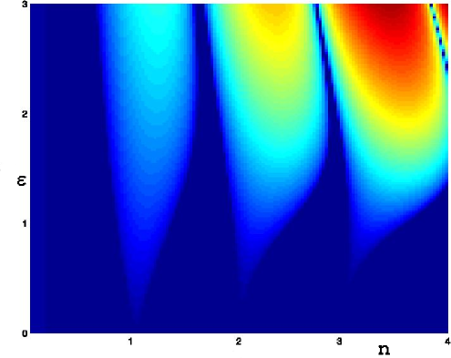
Figure 1: (Figures online colour at www.an-journal.org) Stability regions for the Mathieu equation: on the horizontal axis there is the order of resonance, while the vertical axis describes the strength of the coupling $\epsilon$. The blue region (the external one) is stable, the other colours represent the unstable solutions; the boundary between the two corresponds to the combinations of frequencies and $\epsilon$ that give the steady-state solution (courtesy of V. Karas).

An autoparametric system is one in which the time variation of the system parameters is not explicit, but depends on the coupling of the non-linear terms in different directions. In this context we will use the term parametric resonance to refer to both kind of systems.

3.1 Regions of non-linear resonance

The first result which can be derived by using any perturbative method is that in the approximate solution there are terms with the denominators of the form $n\omega_{r}-m\omega_{z}$ (with $n$ and $m$ being integers). These $n$ and $m$ cannot take any value, but they depend on the symmetry of the metric and of the perturbation: for a plane symmetric configuration one can demonstrate (e.g. Rebusco 2004) that $m=2\>p$ ($p$ integer). Due to this, the regions where $n\omega_{r}=2p\omega_{z}$ are candidate regions of parametric resonance (an analogous reasoning can be done for external resonance).   These systems are well studied in engineering, where usually the main aim is to control the excited resonances: one can find examples of such couplings in aviation (e.g. the problem of how to reduce the vibrations due to rotor blade flapping motion of helicopters), building (e.g. how the elevator ropes respond to high-rise buildings excitations), electronic circuits, etc.

As it can be seen from Fig. 2 of Abramowicz (2005), in General Relativity the epicyclic frequencies are different ($\omega_{z}>\omega_{r}\>\>\forall r$) and there are specific radii at which they are commensurate: hence at those radii an internal resonance between the radial and the vertical direction can occur. The lower order resonance are stronger and more probable: the minimum value for $p$ is $p=1$, hence for a particle in a plane-symmetric strong field the resonance which is most likely to be excited is the $3:2$ ($n=3$, because $n=1,2$ correspond to $\omega_{z}\leq\omega_{r}$ ). When the excitation of one mode reaches a critical amplitude, then the linear response saturates, loses stability and the energy is transferred to the other mode and back. Apart from the distance from the central object, other conditions for the resonance are obviously that the damping does not avoid the growth of the amplitudes and that the perturbation is not too strong (this would lead the system to a chaotic state): these conditions are natural requirements.

In a real accretion disk the perturbation from the whole disk would get excited at the $r_{3:2}$ radius (radius at which the eigenfrequencies are in $3:2$ ratio) and from there a wave would propagate through the whole disk (presumably with lower amplitudes). A $3:2$ resonance was discovered in the planet Mercury: however in that case it is an external resonance between the spin of the planet itself and its orbit around the Sun (Goldreich & Peale $1966$).

3.2 Frequency corrections and the Bursa line

The solution which can be obtained with the method of Poincaré is a special solution, the so called steady-state solution (constant amplitudes and frequencies): this solution is such that also if the frequencies are corrected, their ratio remains exactly $3:2$ (Horák 2004). On the plane ratio versus $\epsilon$ (see Fig. 1) the steady-state solution are the contours which divide the stable solutions (outer part) from the unstable ones (inner part). In a $j$-dimensional system instead of a line, there can exist a $j$-dimensional surface in which the solutions are steady-state. More intersetting solutions are those which are steady up to a certain order of approximation, but vary at higher order: these would be solutions close to the stable surface. We contemplated the possibility of a solution which is steady-state up to the third order, but which is allowed to vary starting from the next order. This would mean that the frequencies:

$$\omega_{r}^{*} = \omega_{r}+\epsilon^{2}\omega_{r}^{(2)}+\epsilon^{3}\omega_{r}^{(3)}+O(\epsilon^{4})\>\>\>,$$

$$\omega_{z}^{*} = \omega_{z}+\epsilon^{2}\omega_{z}^{(2)}+\epsilon^{3}\omega_{z}^{(3)}+O(\epsilon^{4})$$ (4)

and the amplitude of oscillations are constant for $t\sim\epsilon^{(-3)}$, but for longer times they change periodically (Horák 2004), exchanging energy (amplitudes are anticorrelated, frequencies are related). The dominant corrections $\omega_{i}^{(2)}$ depend quadratically on the amplitudes and they are due to the non-linearity. Hence for the observed frequencies we use the relation:

$$\omega_{z}^{*}=S\omega_{r}^{*}+Q,$$ (5)

where $S$ depends quadratically on the amplitudes of the perturbation. In the case studied by Abramowicz et al. (2003) and Rebusco (2004), $S=S(r_{0},\delta r,\delta\theta,\alpha)$. In the above mentioned papers the initial conditions of the perturbed geodesics were found in order to match the observed frequency-frequency slope of the neutron star source Sco X-1. Indeed neutron star sources display different centroid frequencies in different observations, but amazingly they all fit on the same line, which is close to $3:2$. In the numerical study (Abramowicz et al. 2003) this was obtained by changing the initial radius $r_{0}$ and by using the $\alpha$ which gave the strongest response. In the analytical study (Rebusco 2004) the same result was obtained by fixing $\alpha$ and varying the initial perturbations ($\delta r$ and $\delta\theta$). The two procedures agree on the point that a weak perturbation to a free particle leads to quasi-harmonic oscillations, whose frequencies and ratio are close to the eigenfrequencies and to $3:2$ respectively (see Fig. 2; we refer to the deviation from $3:2$ as the Bursa line). Consider the case of BHs and NSs: the mass of the first is greater, hence $\omega_{\rm BH}<\omega_{\rm NS}$. Moreover, suppose that the entity of the perturbation in the two classes of objects is different: if it is stronger in NSs than in BHs, then both the frequency corrections and the observed ratio will be greater in NSs (they are proportional to the square of the amplitudes). The weak point in is this model is that it cannot explain why the slope is $S=0.92$ for all NS sources, rather than a different value: with our simplifications we cannot discriminate the value of $S$, which depends on our choice concerning the perturbation. In principle we cannot even justify why the slope-slope relation is linear! One may infer that this deals with the structure of NSs themselves: in the equations that describe the disk oscillations, there must be a limit cycle, such that for different initial conditions the frequency range changes, but at each time the frequencies fall on the same line. Such limit cycle should be connected to the mass accretion rate in the inner part of the disk.

We emphasize however that in the non-linear resonance model the frequencies shift arises naturally, as well as the deviations from the exact commensurate ratio: this behaviour agrees with the observations. The actual challenge for theoreticians is a full understanding of the “Bursa line”, both qualitatively and quantitatively.

4 Qualitative discussion on other effects

4.1 Frequency-frequency slope: BHs and NSs

The strength of the perturbation is greater in NS than in BH sources: as a consequence the observed frequencies wander much more for NS than in BH ($\omega_{\rm NS}^{(2)}>\omega_{\rm BH}^{(2)}$ ).

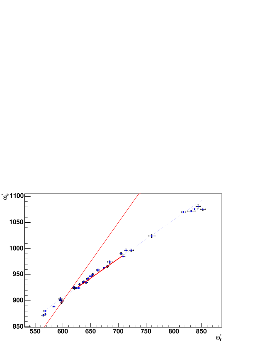
Figure 2: The dotted line is the least-squares best-fit to the data points (the observed kHz QPOs frequencies in Sco X-1), which we call “Bursa line”; the thin solid line corresponds to a slope of $3:2$ (for reference) . The thick solid segment is the analytic approximation, in which the frequencies are scaled for comparison with observations.

However this explanation is not completely satisfactory. The observed signal is not a direct mirror of the disk oscillation, but one has to take into account the propagation and emission mechanisms. In black holes the presence of the event horizon avoids any additional modulation: one can assume that the emitting flux has the characteristic frequencies of the most excited resonance ($r_{3:2}$), and that a subsequent modulation is just due to relativistic effects, such as strong gravitational lensing and Doppler effect (Bursa et al. 2004). Hence the timing properties of the observed photons would be essentially distributed around the frequency of oscillation of a single particle situated at a distance $r_{3:2}$ from the central object. In neutron stars the modulation, which originates in the disk, propagates to the boundary layer (Abramowicz, Horák & Kluźniak 2005; Gilfanov, Revnivtsev & Molkov 2003) and there the original frequencies of oscillation (the ones at $r=r_{3:2}$) are subject to the influence of the Roche lobe overflow: eventually in this case it is difficult to predict how the observed frequencies are related to the original ones (see Horák 2005).

4.2 The effect of a periodic forcing

It is widely accepted that in NS sources the QPO frequencies depend on the spin: this indicates that the the NS spin directly excites the disk oscillations (see Lee 2005 and Sramkova 2005 for numerical results). Let us add external forcing terms to our equations: $A\cos{\omega_{0}t}$ and $B\cos{\omega_{0}t}$. In order to study them with a perturbative method it is convenient to introduce $\tilde{A}$ and $\tilde{B}$ such that $A=\epsilon^{j}\tilde{A}$ and $B=\epsilon^{k}\tilde{B}$ ($j$ and $k$ are integers: they can be different to take into account a different forcing in the two directions).

By considering this forcing a new whole range of resonance conditions is possible:

$$n\omega_{z}\pm m\omega_{r}=q\omega_{0},$$ (6)

with $n,m,q=0,1,2,...\,$. An interesting example was studied by Kluźniak et al. (2004): indeed the combination of frequencies such that the QPOs are separated by $\frac{1}{2}$ the spin frequency would explain the recent observations of the millisecond pulsar SAX J1808.4-3658 (Wijnands et al. 2003). Another possibility in agreement with the data from NS, is that the difference of the QPOs peaks remains locked at the spin frequency itself.

4.3 MRI Turbulence

In the analytical study the turbulence terms were set to zero: up to now only a numerical study of these stochastic differential equations (SDEs) have been done. Anyway from the first experiments (private communication with R. Vio and H. Madsen) we can already see that if a Gaussian noise is assumed, its standard deviation cannot be too large, or the resonance regime will be disrupted in favour of a chaotic one. However for small standard deviations the turbulence introduces new resonances and it drives the system from one stable resonance to the other. The study of these SDEs is very promising: it is necessary to take into account these terms in order to compare our model with observations.

The stochastic terms permit to analyze new behaviours and hopefully their study will lead to a better understanding of the MRI itself.

5 Conclusions

In weakly non-linear oscillators the leading terms are periodic, with frequencies close to the eigenfrequencies of the system: the frequency shift is proportional to the square of the amplitude of the perturbation. The internal coupling of two or more subsystems introduces the possibility of parametric resonances to occur (in the regions where the characteristic frequencies are commensurate). Another feature of non-linear resonance is the presence of subharmonics.

All this suggests that the observed kHz QPOs are a non-linear phenomenon. With the simple toy-model of a perturbed test particle in the strong gravitational field of compact objects, we can qualitatively explain the position of the twin QPO peaks in a frequency-frequency plane. However many puzzles remain to be solved: is there a limit cycle in the system? Is the presence of the boundary layer sufficient to justify the differences between NSs and BHs? Are the shift and the slope of the Bursa line related? How does turbulence affect the resonance conditions? Attacking these questions with the different instruments of theory, computation and observations may lead to a better understanding of the physics of accretion, of the mathematics of non-linear systems, and to the test of strong gravity itself.

- [1] Abramowicz, M.A., Kluźniak, W.: 2001, A&A 374, L19
- [2] Abramowicz, M.A., Karas, V., Kluźniak, W., Lee, W.H., Rebusco, P.: 2003, PASJ 55, 467
- [3] Abramowicz, M.A., Kluźniak, W.: 2003, GReGr 35, 69
- [4] Abramowicz, M.A., Horák, J., Kluźniak, W.: 2005, A&A, in preparation
- [5] Abramowicz, M.A., et al.: 2005, A&A, in preparation
- [6] Bursa, M., Abramowicz, M.A., Karas, V., Kluźniak, W.: 2004, ApJ 617, 45
- [7] Gilfanov, M., Revnivtsev, M., Molkov, S.: 2003, A&A 410, 217
- [8] Goldreich, P., Peale, S.: 1966, AJ 71, 6
- [9] Horák, J.: 2004, in: S. Hledík, Z. Stuchlík (eds.), Processes in the Vicinity of Black Holes and Neutron Stars, Silesian University Opava (astro-ph/0408092)
- [10] Kluźniak, W., Abramowicz, M.A., Kato, S., Lee, W.H., Stergioulas, N.: 2004, ApJ 603, L89
- [11] Méndez, M., van der Klis, M.: 2000, MNRAS 318, 938
- [12] Mook, D.A., Nayfeh, A.H.: 1976, Nonlinear oscillations, John Wiley& Sons, New York
- [13] Poincaré, H.: 1882, Les methodes nouvelles de la mecanique céleste, Gauthiers-Villars, Paris
- [14] Rebusco, P.: 2004, PASJ 56, 553
- [15] Strohmayer, T.E.: 2001, ApJ 552, L49
- [16] van der Klis, M.: 2000 ARA&A 38, 717
- [17] Wijnands, R., van der Klis, M., Homan, J., et al.: 2003, Nature 424, 44