The Evolution of the Broad-Line Region among SDSS Quasars

Based on 5344 quasar spectra taken from the SDSS Data Release 2, the dependences of various emission-line flux ratios on redshift and quasar luminosity are investigated in the ranges $2.0\leq z\leq 4.5$ and $-24.5\geq M_{B}\geq-29.5$. We show that the emission lines in the composite spectra are fitted better with power-law profiles than with double Gaussian or modified Lorentzian profiles, and in particular we show that the power-law profiles are more appropriate to measure broad emission-line fluxes than other methods. The composite spectra show that there are statistically significant correlations between quasar luminosity and various emission-line flux ratios, such as Nv/Civ and Nv/Heii, while there are only marginal correlations between quasar redshift and emission-line flux ratios. We obtain detailed photoionization models to interpret the observed line ratios. The correlation of line ratios with luminosity is interpreted in terms of higher gas metallicity in more luminous quasars. For a given quasar luminosity, there is no metallicity evolution for the redshift range $2.0\leq z\leq 4.5$. The typical metallicity of BLR gas clouds is estimated to be $Z\sim 5Z_{\odot}$, although the inferred metallicity depends on the assumed BLR cloud properties, such as their density distribution function and their radial distribution. The absence of a metallicity evolution up to $z\sim 4.5$ implies that the active star-formation epoch of quasar host galaxies occurred at $z\ga 7$.

1 Introduction

Quasars are among the most luminous objects in the universe and therefore they can be detected and investigated in detail even at very high redshifts, up to $z>6$ (Fan et al. 2001, 2003, 2004). As a consequence, they have been frequently used as a tool to pursue the exploration of the distant universe, such as the investigation of the intergalactic matter (see, e.g., Rauch 1998 for a review), the cosmic re-ionization history (e.g., Fan et al. 2002; Gnedin 2004) and the metal-enrichment history in the universe. Since the gas in the broad-line region (BLR) of quasars is most likely photoionized, as suggested by reverberation mapping observations (e.g., Peterson 1993), it is possible to investigate the chemical composition of gas clouds in BLRs by comparing spectroscopic data with photoionization model calculations. The gas-phase elemental abundances are determined by the star-formation history of the galaxies, therefore studies on the metallicity of BLR in distant quasars are highly insightful of the metal-enrichment history and the galaxy formation in the very early universe (e.g., Matteucci & Padovani 1993; Hamann & Ferland 1993, 1999; Venkatesan et al. 2004). Note that the analysis on the gas metallicity of high-$z$ galaxies not hosting AGN are extremely difficult and time-consuming, because even the brightest galaxies are much fainter than quasars at the same redshift (but see, e.g., Teplitz et al. 2000; Kobulnicky & Koo 2000; Pettini et al. 2001).

It has been often claimed that the gas metallicity of the BLR in quasars is higher than solar (e.g., Baldwin & Netzer 1978; Hamann & Ferland 1992; Ferland et al. 1996; Dietrich et al. 1999, 2003). The inferred metallicity is sometimes very high, several times solar, and for the most extreme case QSO 0353–383 it reaches as much as $Z_{\rm BLR}\sim 15Z_{\odot}$ (Baldwin et al. 2003). Since such high metallicities require deep gravitational potentials and intense star-forming activity in the host galaxies, they provide strong constraints on the evolutionary scenarios of quasar host galaxies (e.g., Hamann & Ferland 1993, 1999; Di Matteo et al. 2004). Another surprising result is that the BLR metallicity does not appear to decrease at the highest redshift proved so far (e.g., Pentericci et al. 2002; Dietrich et al. 2003; Maiolino et al. 2003). This finding gives tight constraints on the first epoch of star formation in the host galaxies, especially when the minimum timescale required for the enrichment of some metals (C, Si, Fe and so on) is taken into account. On the other hand, some observations suggest that quasars at higher-$z$ show higher metallicity than lower-$z$ quasars (e.g., Hamann & Ferland 1992, 1993, 1999). It is also recognized that the BLR metallicity tends to be higher in more luminous quasars (e.g., Hamann & Ferland 1993, 1999). This trend may suggest a connection between the BLR metallicity of quasars and evolutionary processes of the host galaxies. However, since higher-luminosity quasars tend to be selectively observed at higher-$z$, it is not clear how the BLR metallicity depends on the luminosity and redshift, individually.

To investigate the BLR metallicity and understand the chemical evolution of quasars and their host galaxies, it is thus necessary to observe a large number of quasars with sufficiently large ranges of luminosity and redshift. Francis & Koratkar (1995) compared the rest-UV spectra of quasars at the local universe observed with IUE with those at $1.7<z<3.3$ obtained by Large Bright Quasar Survey (LBQS; Foltz et al. 1987) and found little redshift evolution of the UV spectra. Dietrich et al. (2002) investigated the spectra of a larger sample of quasars at $0<z<5$ spanning  6 orders of magnitude in luminosity, based on the data compilation of various observations that were performed with IUE, HST, and some ground-based observatories. However, to avoid possible systematic uncertainties, it is crucially important to use large homogeneous samples of quasars obtained by the same instrument and manner. Thanks to the public data release of the Sloan Digital Sky Survey (SDSS) project (York et al. 2000), spectra of more than a few thousands quasars are now available, and therefore a systematic examination of BLR properties becomes feasible. Although the signal-to-noise ratio of each spectrum in the SDSS database is not high enough to measure emission-line fluxes accurately, higher quality spectra can be obtained by the “composite” of numerous individual spectra. Composite spectra are a very efficient tool not only to increase the data quality, but also to minimize effects due to individual characteristics of each quasars. Note that the datasets of the 2dF and 6dF QSO Redshift Surveys (e.g., Croom et al. 2004) are also available to examine various statistical properties of quasars (e.g., Croom et al. 2002); however, most quasars found by these surveys are only at $z<3$ and the spectra are not calibrated in (relative) flux, making it difficult to obtain accurate emission-line flux ratios. By using composite SDSS spectra, various spectroscopic properties of quasars have already been investigated, such as the spectral energy distribution (SED) (Vanden Berk et al. 2001) and broad absorption line (BAL) objects (Reichard et al. 2003a). The purpose of this paper is to use composite spectra of SDSS quasars to derive the dependences of BLR emission-line spectra on redshift and luminosity in wide ranges, although the luminosity range is narrower for high-redshift quasars due to the limited spectroscopic sensitivity of the SDSS dataset.

In this paper, we present our making of the composite spectra of SDSS quasars for various redshift and luminosity intervals. The measured emission-line flux ratios and other spectroscopic properties are discussed in detail. By combining these observational results with new extensive photoionization models, we investigate the metallicity and other spectroscopic properties of the BLRs. Throughout this paper, we adopt a cosmology with ($\Omega_{\rm tot}$, $\Omega_{\rm M}$, $\Omega_{\Lambda}$) =(1.0, 0.3, 0.7) and $H_{0}$ = 70 km s^-1 Mpc^-1 .

2 Composite spectra

2.1 Spectral composition

The spectroscopic data of SDSS quasars (Richards et al. 2002a) were obtained from the SDSS archive, Data Release 2 (DR2; Abazajian et al. 2004). The spectral resolution of the SDSS spectroscopic data is $\sim$2000, that corresponds to $\Delta v\sim 150$ km s^-1, which is high enough for our scientific purposes. Only quasars at $2.0\leq z\leq 4.5$ are considered in this paper, because in this redshift range the wavelength coverage of the SDSS spectroscopic data ($3800{\rm\AA}\la\lambda_{\rm obs}\la 9200{\rm\AA}$) includes at least the rest frame wavelength interval from Ly$\alpha$ $\lambda$1216 to He ii $\lambda$1640. There are 6181 quasars within this redshift range and with a redshift confidence level of zConf $\geq$ 0.75 in the DR2 archive; while 311 objects are excluded because not matching this zConf criterion. 109 objects are removed from the 6181 quasars: 84 spectra of them suffer from bad focusing of the spectrograph collimator and 25 spectra suffer from leaking light from a LED (see Abazajian et al. 2004 for more details). Therefore the number of usable quasar spectra is 6072. Note however that this sample is not a complete one in any sense, because the spectroscopic targets are selected heterogeneously: some of them are selected through their SDSS photometric properties, and others are selected by cross-identification with radio or X-ray sources.

The SDSS quasar selection algorithm picks up not only “normal” quasars, but also broad absorption line (BAL) quasars (Richards et al. 2002a). Indeed Reichard et al. (2003b) found 224 BAL quasars among 3814 quasars in the SDSS early data release (EDR; Stoughton et al. 2002). BAL quasars should be removed because the BAL features affect fluxes and profiles of broad emission lines in the composite spectra, therefore we removed BAL quasars from our sample. Here we did not adopt the standard “Balnicity Index (BI)” (Weymann et al. 1991) to identify BAL quasars. This is because BI does not identify quasars with a strong absorption line close to the systemic velocity of the quasar ($\mid\!\!v_{\rm outflow}\!\!\mid<3000$ km s^-1), by definition. For our purpose, however, quasars with such associated absorption lines (see, e.g., Foltz et al. 1986) should be also removed to investigate the BLR emission-line properties correctly. We checked all of the 6072 quasars by eye and identified 724 quasars with strong absorption features, which were removed from our quasar sample.

Each spectrum was then corrected for Galactic reddening with the reddening curve of Cardelli et al. (1989), even though the effect is very small in most cases because the SDSS survey area is at high Galactic latitude, i.e. $E(B-V)<0.05$ mag for $\sim 83\%$ and $E(B-V)<0.10$ mag for $\sim 98\%$ of our sample [the median value is $E(B-V)=0.029$ mag]. Note that the spectroscopic data in the EDR archive and the DR1 archive are already corrected for the Galactic reddening, which is different from the spectroscopic data in the DR2 archive. The $k$-correction for each quasar was applied for calculating the absolute $B$ magnitude. For this purpose, a simple power-law SED with a power-law index of $\alpha=0.5$ (where $f_{\nu}\propto\nu^{-\alpha}$) is assumed for the intrinsic spectral shape of quasars, following other studies on SDSS quasars (e.g., Schneider et al. 2002, 2003). This assumption seems valid at least at $\lambda_{\rm rest}<5000{\rm\AA}$, based on the composite spectrum of the whole SDSS quasar sample (Vanden Berk et al. 2001). In this study, the absolute magnitude of quasars was calculated from the $i^{\prime}_{\rm PSF}$ magnitude, because an $i^{\prime}$-band flux is not affected by the Lyman-break for quasars at $z\leq 4.5$.

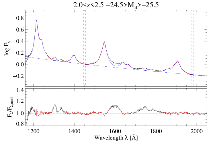
Figure 1: ($Upper$) Composite spectrum of quasars with $-24.5>M_{B}\geq-25.5$ and $2.0\leq z<2.5$, and the fitting result (blue line). For the composite spectrum, the wavelength parts which are used to the fitting are shown in red while the wavelength parts which are excluded from the fitting process are shown in black. The spectral regions denoted by vertical dotted lines are used to determine the initial guess of the continuum level and slope in the fitting process. The initial guess and the fitted power-law continuum are denoted by blue dotted and dashed lines, respectively. ($Lower$) Residual of the model fitting. Again the red parts of the data denote the wavelength regions used in the model fitting, and the black parts denote the excluded spectral regions in the model fitting. The excesses drawn by a blue, green, and yellow lines identify Oi+Siii $\lambda$1305, Cii$\lambda$1335, and 1600${\rm\AA}$ bump, respectively.

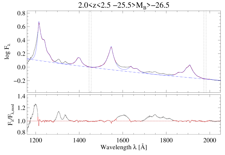
Figure 2: Same as Figure 1 but for the composite spectrum of quasars with $-25.5>M_{B}\geq-26.5$ and $2.0\leq z<2.5$.

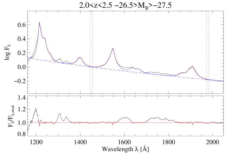
Figure 3: Same as Figure 1 but for the composite spectrum of quasars with $-26.5>M_{B}\geq-27.5$ and $2.0\leq z<2.5$.

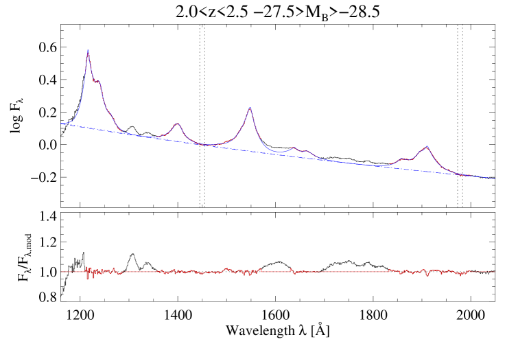
Figure 4: Same as Figure 1 but for the composite spectrum of quasars with $-27.5>M_{B}\geq-28.5$ and $2.0\leq z<2.5$.

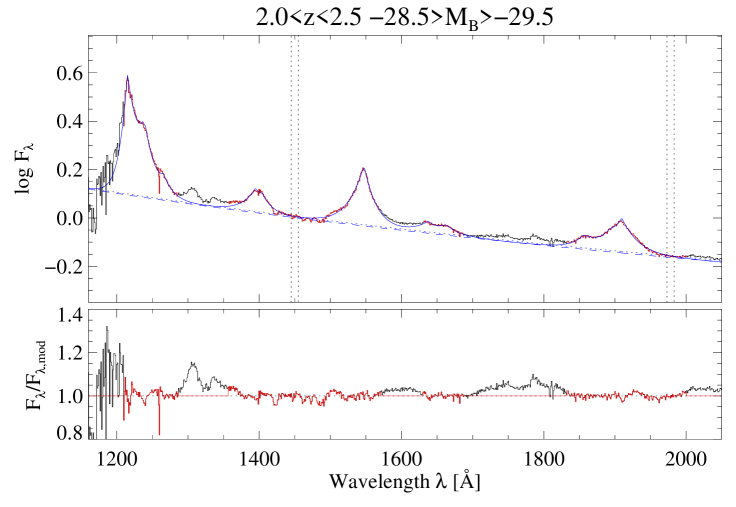
Figure 5: Same as Figure 1 but for the composite spectrum of quasars with $-28.5>M_{B}\geq-29.5$ and $2.0\leq z<2.5$.

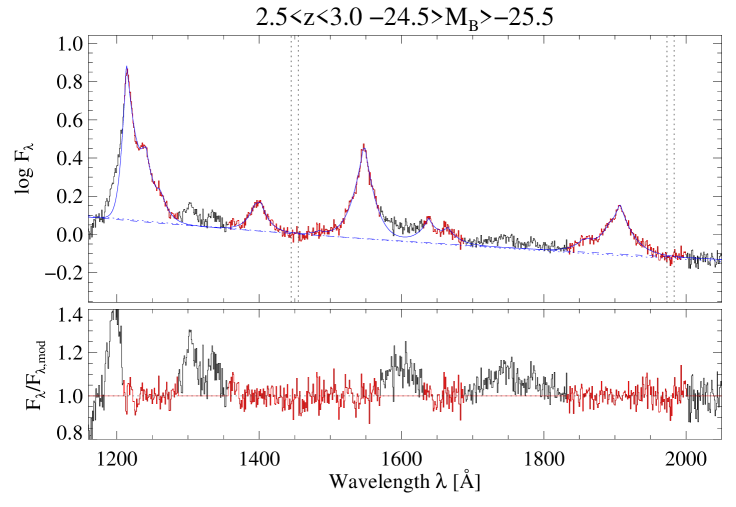
Figure 6: Same as Figure 1 but for the composite spectrum of quasars with $-24.5>M_{B}\geq-25.5$ and $2.5\leq z<3.0$.

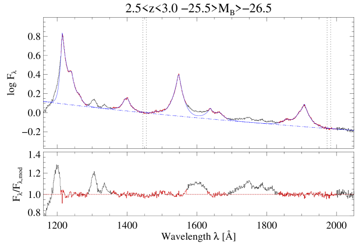
Figure 7: Same as Figure 1 but for the composite spectrum of quasars with $-25.5>M_{B}\geq-26.5$ and $2.5\leq z<3.0$.

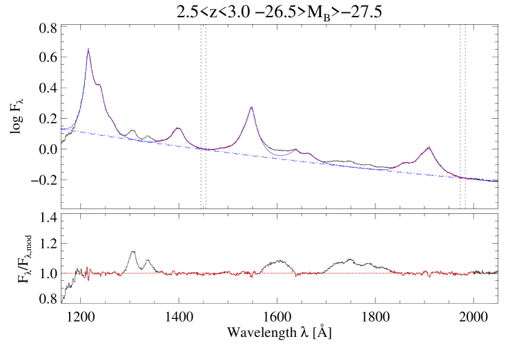
Figure 8: Same as Figure 1 but for the composite spectrum of quasars with $-26.5>M_{B}\geq-27.5$ and $2.5\leq z<3.0$.

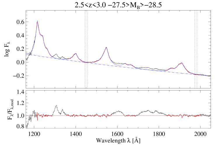
Figure 9: Same as Figure 1 but for the composite spectrum of quasars with $-27.5>M_{B}\geq-28.5$ and $2.5\leq z<3.0$.

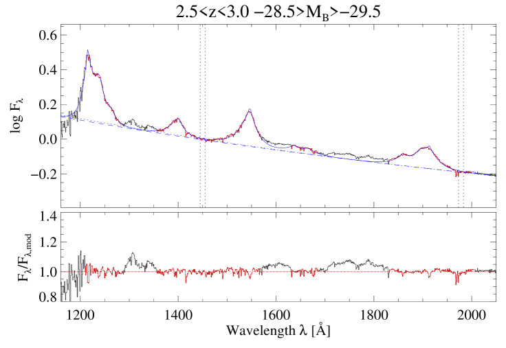
Figure 10: Same as Figure 1 but for the composite spectrum of quasars with $-28.5>M_{B}\geq-29.5$ and $2.5\leq z<3.0$.

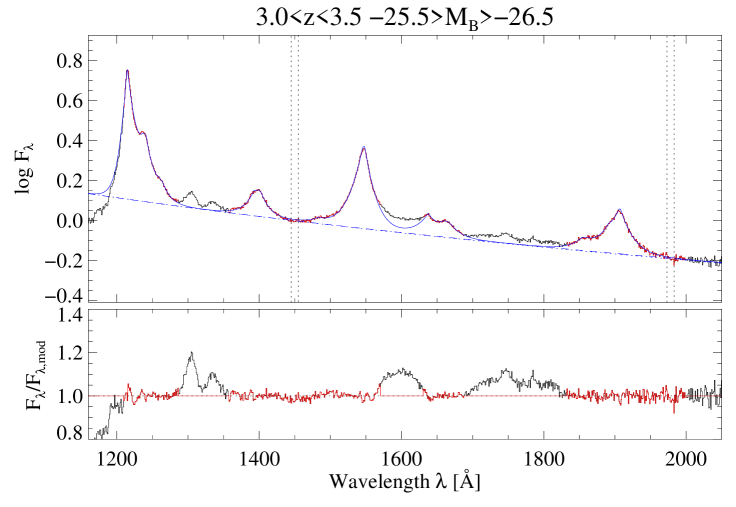
Figure 11: Same as Figure 1 but for the composite spectrum of quasars with $-25.5>M_{B}\geq-26.5$ and $3.0\leq z<3.5$.

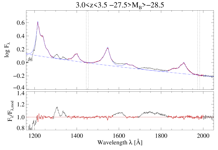
Figure 13: Same as Figure 1 but for the composite spectrum of quasars with $-27.5>M_{B}\geq-28.5$ and $3.0\leq z<3.5$.

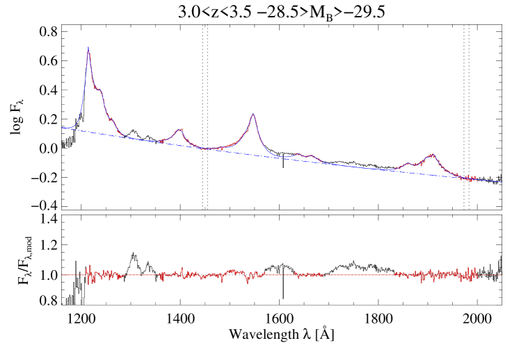
Figure 14: Same as Figure 1 but for the composite spectrum of quasars with $-28.5>M_{B}\geq-29.5$ and $3.0\leq z<3.5$.

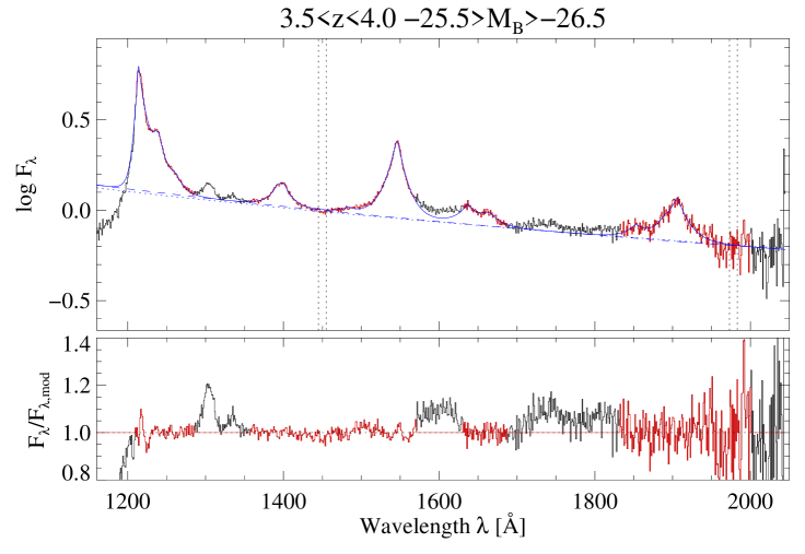
Figure 15: Same as Figure 1 but for the composite spectrum of quasars with $-25.5>M_{B}\geq-26.5$ and $3.5\leq z<4.0$.

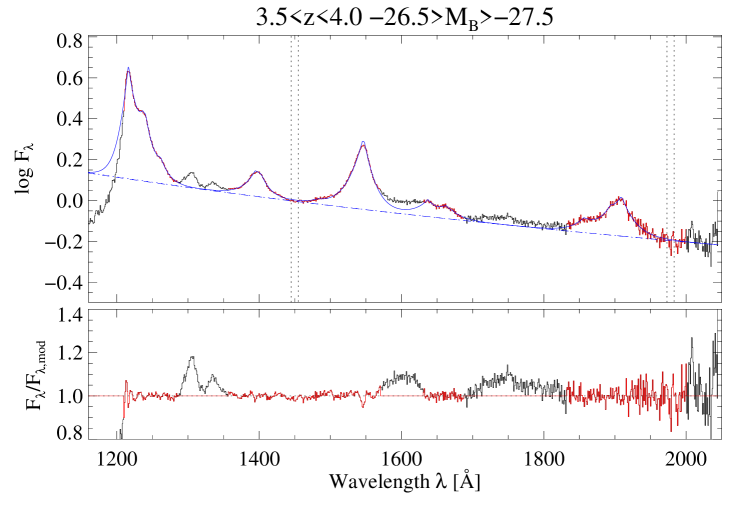
Figure 16: Same as Figure 1 but for the composite spectrum of quasars with $-26.5>M_{B}\geq-27.5$ and $3.5\leq z<4.0$.

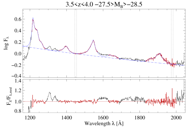
Figure 17: Same as Figure 1 but for the composite spectrum of quasars with $-27.5>M_{B}\geq-28.5$ and $3.5\leq z<4.0$.

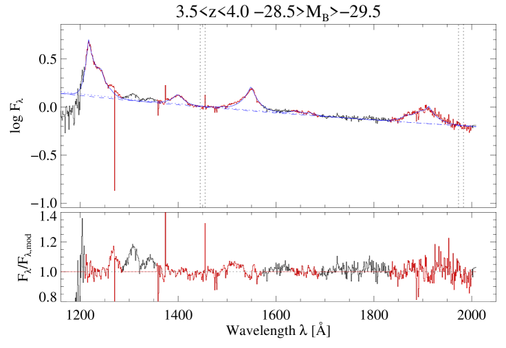
Figure 18: Same as Figure 1 but for the composite spectrum of quasars with $-28.5>M_{B}\geq-29.5$ and $3.5\leq z<4.0$.

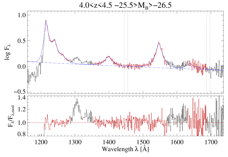
Figure 19: Same as Figure 1 but for the composite spectrum of quasars with $-25.5>M_{B}\geq-26.5$ and $4.0\leq z<4.5$.

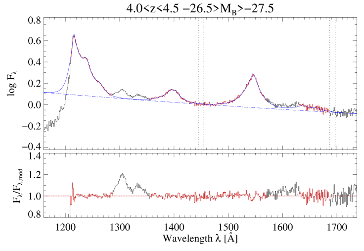
Figure 20: Same as Figure 1 but for the composite spectrum of quasars with $-26.5>M_{B}\geq-27.5$ and $4.0\leq z<4.5$.

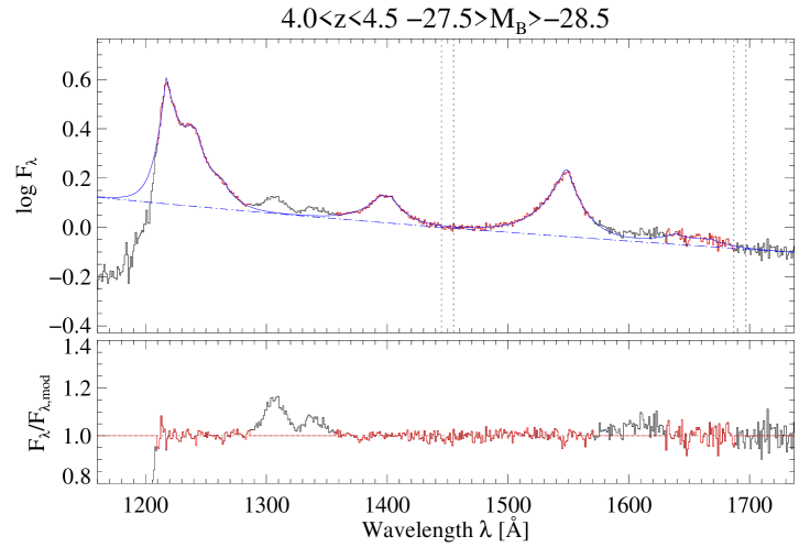
Figure 21: Same as Figure 1 but for the composite spectrum of quasars with $-27.5>M_{B}\geq-28.5$ and $4.0\leq z<4.5$.

For most of the quasars in our sample, the signal-to-noise ratio of the individual spectra is not high enough to measure the properties of the broad emission lines accurately. However, as mentioned above, we can investigate the BLR properties as a function of redshift and quasar luminosity by constructing composite spectra of quasars in certain parameters ranges and by examining the BLR properties in such composite spectra. As discussed by Vanden Berk et al. (2001), there are mainly two methods to combine the spectroscopic data. One is the arithmetic mean method, which preserves the relative fluxes of emission features. The other is the geometric mean method, which preserves global continuum shapes. Since we are interested mainly in broad emission-line properties and not in global continuum SED, we adopt the former strategy to combine the quasar spectra. However, the choice of the composite method does not affect results and discussion significantly: the measured emission-line fluxes vary less than 10% if we adopt the geometric mean instead of the arithmetic mean. The spectral composition was performed by using the IRAF task, scombine, adopting a 5$\sigma$ clipping rejection criterion to remove bad pixels. Before combining the spectral data, it is necessary to shift the data from the observed frame to the quasar rest frame. However, the accurate determination of quasar redshifts is not an easy task, because broad emission lines tend to be shifted blueward or redward compared to the quasar rest frame (e.g., Gaskell 1982; Richards et al. 2002b). Although narrow emission lines are sometimes used as a measure of systemic recession velocities of quasars (e.g., Vanden Berk et al. 2001), we cannot use narrow emission lines because only the rest-frame ultraviolet spectral region (which lacks of narrow lines) is available due to the redshift range of the sample. Despite this uncertainty, we simply adopted the redshift assigned by the SDSS reduction pipeline. This choice is acceptable for us because we are mainly interested in the broad emission-line flux ratios, but it should be kept in mind that a consequence may be non-negligible uncertainties in the velocity profiles of emission lines in the composite spectra. We will discuss this issue briefly in §§4.1. After shifting the spectra to the quasar rest frame, the data were re-binned to a common dispersion of 1 ${\rm\AA}$. Then each individual spectrum was normalized to the mean flux density at $1445{\rm\AA}<\lambda_{\rm rest}<1485{\rm\AA}$. In this normalization process, 4 objects were removed from the 5348 objects because their spectra show significant problems in the wavelength range of $1445{\rm\AA}<\lambda_{\rm rest}<1485{\rm\AA}$. As a consequence the number of quasars used in the following analysis is 5344. Then the quasars are divided into redshift and luminosity bins with the intervals of $\Delta z=0.5$ and $\Delta M_{B}=1$ mag. In Table 1 the final number of objects used in our analysis is given for each redshift and luminosity bin. Among the composite spectra, we analyze only those which were created by at least 5 individual spectra. The resulting composite spectra are shown in Figures 1–21.

2.2 Emission-line measurement: the method

The measurement of emission-line fluxes in quasar spectra is a complicated issue, both because some adjoining emission-line such as “Ly$\alpha$ and Nv$\lambda$1240” and “Aliii$\lambda$1857, Siiii]$\lambda$1892 and Ciii]$\lambda$1909” are heavily blended, and also because the continuum level is often not easy to estimate. There are two methods which have been employed mostly. One is by fitting the detected emission-line feature by some appropriate function, and the other is by defining a “local” continuum level for each emission line and integrating the flux above the adopted continuum level. Zheng et al. (1997) adopted the former method to measure emission-line fluxes in the composite HST quasar spectrum through multiple Gaussian fitting (see also, e.g., Laor et al. 1994). Vanden Berk et al. (2001) adopted the latter strategy and measured line fluxes in the composite spectrum of 2204 SDSS quasars spanning a wide luminosity and redshift range by summing up the line flux above a defined local continuum level. Here it should be kept in mind that both methods have serious difficulties to measure accurate emission-line fluxes. As for the profile-fitting method, it is crucial to choose appropriate functions to fit emission lines. A simple Gaussian or Lorentzian profile does not work since the broad emission lines of quasars generally show asymmetric velocity profiles (e.g., Corbin 1997; Vanden Berk et al. 2001; Baskin & Laor 2005). Although the multi-Gaussian method can achieve reasonably sufficient profile fit, it requires many free parameters. It is also reported that the best-fit profile function may depend on the velocity width and other AGN properties (e.g., Sulentic et al. 2002). As for the local-continuum method, on the other hand, it is not clear whether the adopted continuum level is appropriate or not; this uncertainty may be crucial especially when blended emission lines are concerned.

In this work, we adopt the profile-fitting method because we are interested in the fluxes of emission lines including heavily blended ones, such as Nv$\lambda$1240, which is generally regarded as an important metallicity diagnostic (e.g., Hamann & Ferland 1993; Hamann et al. 2002). The following function is adopted to fit the line profiles:

$$F_{\lambda}=\cases{F_{0}\times\left(\frac{\lambda}{\lambda_{0}}\right)^{-\alpha}\ \ \ {\rm for}\ \lambda>\lambda_{0}\cr F_{0}\times\left(\frac{\lambda}{\lambda_{0}}\right)^{+\beta}\ \ \ {\rm for}\ \lambda<\lambda_{0}\cr}$$ (1)

here the power-law indices ($\alpha$ and $\beta$) are different between the blue side and the red side of a given emission line (i.e., $\alpha\neq\beta$ generally), which allows us to fit asymmetric velocity profiles. This function can achieve a better fit than double-Gaussian and modified (i.e., asymmetric) Lorentzian methods (see §§4.1). Since the emission lines with a different ionization degree tend to show systematically different velocity profiles (e.g., Gaskell 1982; Wilkes 1984, 1986; Baskin & Laor 2005), we divide the detected UV emission lines into two main groups: high-ionization lines (HILs; Nv$\lambda$1240, Oiv$\lambda$1402, Niv]$\lambda$1486, Civ$\lambda$1549 and Heii$\lambda$1640) and low-ionization lines (LILs; Siii$\lambda$1263, Siiv$\lambda$1398, Oiii]$\lambda$1663, Alii$\lambda$1671, Aliii$\lambda$1857, Siiii$\lambda$1887 and Ciii]$\lambda$1909), with the boundary ionization potential of $\sim 40$ eV. See, e.g., Collin-Souffrin & Lasota (1988) for a discussion on this dichotomy. For reader’s convenience, the ionization potentials of the concerned ions are given in Table 2. Since emission-line profiles (width, asymmetry, and shift) are correlated with the ionization potential of the corresponding ions (e.g., McIntosh et al. 1999), emission lines with similar ionization degree tend to show similar profiles, approximately. We thus assume that all emission lines in the same group have the same power-law indices of $\alpha$ and $\beta$, and the same wavelength shift of the emission-line center ($\lambda_{0}$) with respect to the systemic velocity. All the line profiles within the same group were fitted simultaneously to infer the best $\alpha$, $\beta$ and $\lambda_{0}$. As for the Ly$\alpha$ profile, we adopt the same red-side index ($\alpha$) as that for HILs and the other parameters are left free; this is to avoid that absorption by intervening IGM on the blue side of Ly$\alpha$ affects the overall fit (as we will discuss later on, we are not interested in the Ly$\alpha$ itself but in Nv$\lambda$1240, which is blended with it). The model fitting is performed in the spectral region at $1210{\rm\AA}<\lambda<2000{\rm\AA}$ except for the composite spectra of quasars at $4.0\leq z<4.5$, for which the fitting is performed at $1210{\rm\AA}<\lambda<1687{\rm\AA}$ due to the smaller (rest-frame) spectral coverage. The slope and the amplitude of the power-law continuum are initially estimated in two wavelength regions where the emission-line contribution to the total flux appears to be small ($1445{\rm\AA}<\lambda<1455{\rm\AA}$ and $1973{\rm\AA}<\lambda<1983{\rm\AA}$) and finally determined by the model fitting. Since the redder emission-line free region is not available for the composite spectra of quasars at $4.0\leq z<4.5$, we refer to a spectral region at $1687{\rm\AA}<\lambda<1697{\rm\AA}$ instead of that at $1973{\rm\AA}<\lambda<1983{\rm\AA}$ for the initial guess of the parameters for the continuum emission.

The Oi+Siii composite at 1305${\rm\AA}$ and Cii$\lambda$1335 is measured simply by summing up all of flux above the continuum level for each line ($1286{\rm\AA}\leq\lambda\leq 1322{\rm\AA}$ for the Oi+Siii composite and $1322{\rm\AA}\leq\lambda\leq 1357{\rm\AA}$ for Cii$\lambda$1335), because their velocity profiles are different from both HILs and LILs. We also measure the flux of a “1600${\rm\AA}$ bump”, which is clearly seen in the residual spectra (see lower panels in Figures 1–21). We simply sum up the flux above the continuum level ($1570{\rm\AA}\leq\lambda\leq 1631{\rm\AA}$) also for this unidentified spectral feature. The nature of the 1600${\rm\AA}$ bump will be discussed in §§4.2. All these spectral regions (Oi+Siii $\lambda$1305, Cii$\lambda$1335, and “1600${\rm\AA}$ bump”) are excluded from the fit. Also, the wavelength region at $1687{\rm\AA}<\lambda<1833{\rm\AA}$ is excluded from the fitting process because there are heavily blended emission lines such as Niv$\lambda$1719, Alii$\lambda$1722, Niii]$\lambda$1750 and Feii multiplets.

2.3 Emission-line measurement: results

The fitting results are shown in Figures 1–21. The measured emission-line fluxes, normalized to the Civ$\lambda$1549 flux, are given in Tables 3–7. Here the errors given in Tables 3–7 contain only the statistical errors, which are estimated from the covariance matrix in the standard way. The measured profile parameters, i.e., the velocity shifts from the systemic velocity, the $\alpha$ and $\beta$ parameters, and the velocity widths in FWHM, are given in Table 8. To see how the BLR emission-line properties depend on redshift and luminosity, some measured emission-line flux ratios are plotted as a function of redshift and absolute $B$ magnitude in Figures 22 and 23. For Siiv$\lambda$1397 and Oiv]$\lambda$1402 only the sum of their flux is considered, because the wavelength separation of those two lines is so small that the fitting process can hardly deblend them for some composite spectra (in Table 3 the measured Oiv]$\lambda$1402 flux is nearly zero only for the brightest case while the Siiv flux increases suddenly at this luminosity). For the same reason, only the sum of the Oiii]$\lambda$1663 and the Alii$\lambda$1671 is plotted in Figures 22 and 23. As shown in Figure 22, there are no apparent redshift dependences in the major emission-line ratios, although the highest-redshift data may deviate from the lower-redshift trend in some flux ratios such as Siii$\lambda$1263/Civ$\lambda$1549, (Oi$\lambda$1304+Siii$\lambda$1307)/Civ$\lambda$1549, and (Oiii]$\lambda$1663+Alii$\lambda$1671)/Civ$\lambda$1549. Figure 22 shows that systematic differences in the emission-line flux ratios at different luminosities are present. This tendency is more clear in Figure 23, where significant correlations between some flux ratios and luminosity are seen.

In order to examine more quantitatively the significance of the correlation of emission-line flux ratios with redshift and luminosity, in Figures 24 and 25 we show the flux ratios normalized to the values measured from the composite spectra at $2.0\leq z<2.5$ or $-26.5>M_{B}\geq-27.5$. For these normalized flux ratios, we apply a linear fit, whose results are also shown in Figures 24 and 25. The slopes of the best-fit results are given in Table 9. We also examine whether the flux ratios are correlated with redshift or absolute $B$ magnitude with a statistical significance, by applying the Spearman rank-order test. The derived Spearman rank-order correlation coefficients ($r_{\rm S}$) and their statistical significance $p(r_{\rm S})$, which is the probability of the data being consistent with the null hypothesis that the flux ratio is not correlated with redshift or absolute $B$ magnitude, are also given in Table 9. The results of the Spearman rank-order test are summarized as follows:

• There are no statistically significant correlations between the examined flux ratios and redshift except for (Oi+Siii)/Civ, which is marginally positively correlated with redshift.

• The flux ratios of Nv/Civ, (Siiv+Oiv)/Civ, Aliii/Civ, Siiii]/Civ and Nv/Heii show statistically significant positive correlations with absolute $B$ magnitude. On the contrary, the flux ratios of (1600${\rm\AA}$ bump)/Civ and Heii/Civ show significant negative correlations with absolute $B$ magnitude.

Note that the possible marginal correlations seen in Figure 24 are mainly due to the data for the highest redshift quasar composite spectra; there are no apparent correlations for those flux ratios in the range $2.0<z<4.0$.

We also examine the dependences of emission-line shifts and FWHMs on redshift and absolute $B$ magnitude. However, as mentioned in §§2.1, the shape of the emission lines may be inaccurate due to the uncertainty in redshift of individual quasars. Therefore we focus on the relative velocity difference between HILs and LILs, which is less affected by uncertainties in the absolute velocity determinations. The relative differences of HILs and LILs in emission-line peaks ($\Delta v_{\rm HIL}-\Delta v_{\rm LIL}$) and FWHMs of HILs and LILs are plotted in Figure 26, as a function of redshift and absolute $B$ magnitude. These profile parameters appear to be strongly correlated with absolute $B$ magnitude while not correlated with redshift. The Spearman rank-order test results in probabilities of the uncorrelation between redshift and emission-line shift, FWHM of HILs and LILs of 0.46, 0.11 and 0.45 respectively, while those between absolute $B$ magnitude and emission-line shift, FWHM of HILs and LILs are $2.5\times 10^{-3}$, $5.3\times 10^{-5}$ and $2.0\times 10^{-2}$. These results indicate that the correlations between absolute $B$ magnitude and emission-line shift and FWHM of HILs are statistically significant while those between redshift and emission-line shift, FWHM of HILs and LILs are statistically uncorrelated. The relations between FWHMs, redshift, and absolute $B$ magnitude are interesting issues since they contains information on the growth of supermassive black holes (SMBHs). We do not discuss this issue further since this topic is beyond the scope of this paper.

3 Photoionization models

3.1 Method

To interpret these results quantitatively, it is very useful to compare emission-line flux ratios with photoionization models. However, it is well known that simple one-zone photoionization models cannot properly describe BLRs because gas clouds in BLRs span wide ranges in densities and/or ionization degrees in general (e.g., Davidson 1977; Collin-Souffrin et al. 1982). To investigate the physical properties of gas clouds in the BLRs of quasars, Baldwin et al. (1995) proposed the locally optimally emitting cloud (LOC) model, which is a multi-zone photoionization model. In this model, gas clouds with a wide range of physical conditions are present at a wide range of distances, and thus the net emission-line spectra can be calculated by integrating in the parameter space of gas density and radius, assuming some distribution functions. This model can predict fluxes of both low-ionization emission lines and high-ionization emission lines consistently and simultaneously, and thus it has been sometimes used to investigate physical and/or chemical properties of ionized gas clouds in BLRs (e.g., Korista et al. 1998; Korista & Goad 2000; Hamann et al. 2002).

Adopting this LOC model, we carried out photoionization model calculations by using the photoionization code $Cloudy$ version 94.00 (Ferland 1997). For simplification, we assume a plane-parallel geometry and a constant gas density for each gas cloud. Dust grains are not included in our calculations because gas clouds in BLRs are thought to be in a dust-free region (e.g., Netzer & Laor 1993) and we have verified that the physical conditions in our grid of models imply dust sublimation in most cases. Those few cases which allow dust survival were excluded from the final calculation, as briefly mentioned also in §§3.2. Our assumption for the chemical composition is the same as that of Hamann et al. (2002), in which the relative metal abundances scale by keeping solar relative values except for nitrogen, which scales as the square power of other metal abundances (see Table 3 of Hamann et al. 2002). Here the solar elemental abundances are taken from Grevesse & Anders (1989) with extensions by Grevesse & Noels (1993). As for the SED of the ionizing photons, two types of SED are adopted to see possible SED effects on the results: one is a SED with a strong UV thermal bump which matches the quasar template of Scott et al. 2004, and the other is with a weak UV thermal bump which matches the HST quasar templates (Zheng et al. 1998; Telfer et al. 2002; see also Marconi et al. 2004 for more details). Both SEDs have the same optical to X-ray ratio $\alpha_{\rm OX}$ (Zamorani et al. 1981; Ferland 1997), i.e., $\alpha_{\rm OX}=-1.49$, but different slopes in the energy range of $9.1{\rm eV}\leq h\nu\leq 35.5{\rm eV}$. See Figure 27 for a graphical representation of the two SEDs (see also Nagao et al. 2005). The calculation for each cloud is stopped when the cloud thickness reaches $10^{23}$ cm^-2 or when the cloud temperature drops below 3000 K. We performed model runs for gas clouds with a gas density ($n$) in the range of $10^{7-14}$ cm^-3 with a 0.2 dex step, with a flux of ionizing photons ($\Phi$) in the range $10^{17}-10^{24}$ cm^-2 s^-1 also with a 0.2 dex step, and with metallicities of $Z/Z_{\odot}$ = 0.2, 0.5, 1.0, 2.0, 5.0 and 10.0. Therefore the number of the performed model runs is 1296 for each metallicity and SED, giving a total number of 15552 runs.

Once the calculations are completed, we can obtain the net emission-line flux by integrating the line emissivity of all clouds; i.e.,

$$L_{\rm line}=\int\!\!\!\int 4\pi r^{2}F_{\rm line}(r,n)\ f(r)g(n)\ dn\ dr$$ (2)

where $f(r)$ and $g(n)$ are the cloud distribution functions for radius and gas density, respectively. Note that the radius is specified by the ionizing photon flux. Baldwin et al. (1995) assumed simple power-law functions for both $f(r)$ and $g(n)$; i.e., $f(r)\propto r^{\Gamma}$ and $g(n)\propto n^{\beta}$. It has been shown that the observed BLR emission-line spectra are generally well reproduced by the LOC models with $\Gamma\sim-1$ and $\beta\sim-1$ (e.g., Baldwin 1997; Korista & Goad 2000).

3.2 Model results

In Figure 28, we present some examples of calculated line emissivities as a function of gas density and ionizing photon flux. Contours indicate the predicted equivalent widths for full geometrical coverage referred to the incident continuum at $1215{\rm\AA}$, for models with ionizing SED with a large UV thermal bump and a metallicity of $Z/Z_{\odot}=1.0$. It should be mentioned that the model calculations for some clouds with certain pair of ($n$, $\Phi$) fail because of a thermal instability effect of the ionized gas (see Ferland 1997 for details of this problem). This problem is more serious when high metallicity gas clouds are examined. However even for the highest-metallicity cases (i.e., $Z/Z_{\odot}$ = 10.0), the fraction of the crashed runs is less than 6% of the 1296 model runs. The line emissivities for the crashed cases are estimated by simple interpolations on the $n$-$\Phi$ plane using the results of the neighboring uncrashed models.

In Figure 29, the net emission-line flux ratios are presented as a function of gas metallicity, which are obtained by the integrations as given in the equation (2). Here we adopt $\Gamma=-1$ and $\beta=-1$, i.e., $f(r)\propto r^{-1}$ and $g(n)\propto n^{-1}$. In the integration procedure, gas clouds with a gas density of $n<10^{8}$ cm^-3 are excluded because such low-density clouds are thought to be implausible for BLRs, which is inferred by the absence of broad [O iii]$\lambda$4363 emission lines in spectra of AGNs (note that the critical density of the [O iii]$\lambda$4363 transition is $n_{\rm crit}=3.3\times 10^{7}$ cm^-3). Gas clouds with an ionizing photon flux of $\Phi<10^{18}$ cm^-2 s^-1 are also excluded, because the energy density temperature of the incident continuum emission for clouds with such a small $\Phi$ falls below 1000 K for our adopted SEDs, at such temperature dust grains may survive and absorb most of the ionizing photons (as well as most of any UV line flux which may be produced; Netzer & Laor 1993). The adopted integration range is thus $8\leq{\rm log}\ n\leq 14$ and $18\leq{\rm log}\ \Phi\leq 24$. The predicted net emission-line flux ratios are also given in Table 10.

As apparent in Figure 29, most of emission-line fluxes normalized to the flux of Civ$\lambda$1549 are positively correlated with the gas metallicity. This is mainly because the Civ$\lambda$1549 transition is an important coolant. This is especially true in metal-poor environments where the cooling by other metal lines is less effective, making Civ$\lambda$1549 emission become stronger when the gas metallicity is lower. The effects of ionizing continuum SED on the resultant predictions are very small, generally far less than a factor of 2. Note that some of the predicted flux ratios are sensitive to the adopted weighting functions, $f(r)$ and $g(n)$, especially when lines with a different ionization degree are concerned (e.g., Cii/Civ). We discuss the effect of this dependence on our results in §§4.2. Note that Hamann et al. (2002) also presented the results of the LOC photoionization model calculations with the same assumption on the relative elemental abundance ratios. Our results are almost consistent with those of Hamann et al. (2002). The small differences may be due to the differences in the adopted SEDs, to the integration ranges of $n$ and $\Phi$, to the version of Cloudy, and to the column density of clouds.

4 Discussion

4.1 Comparison of emission-line fitting methods

Before comparing the results of photoionization model calculations with the measured emission-line flux ratios of SDSS DR2 quasars, we should discuss whether our measurement method is appropriate or not. Our adopted formula for measuring emission lines [equation (1)] is different from the widely adopted formulae such as multi-Gaussian and (modified) Lorentzian. In Figure 30, we compare the fitting results by adopting equation (1), double Gaussian (allowing the different central velocity for the two Gaussian components), and modified Lorentzian that is described by the following formula;

$$F_{\lambda}=\frac{F_{0}}{1+\left(\frac{\lambda-\lambda_{0}}{\Delta\lambda}\right)^{\alpha}}$$ (3)

($\alpha=2$ gives a usual Lorentzian function). Our adopted function provides a much better fit than the double Gaussian and modified Lorentzian; this is apparent especially on the blue side of Civ$\lambda$1549 emission and on the red side of Heii$\lambda$1640 emission. Note that the number of the free parameter in our fitting function is four (amplitude, central wavelength, $\alpha$ and $\beta$) while those of double Gaussian and modified Lorentzian are six and four, respectively. Although multi-Gaussian methods with three or more components may achieve better fit for a single line, they require too many parameters and makes the interpretation more complex. As a consequence, we conclude that our power-law fitting is better than the other methods to describe broad emission-line profiles of quasar composite spectra.

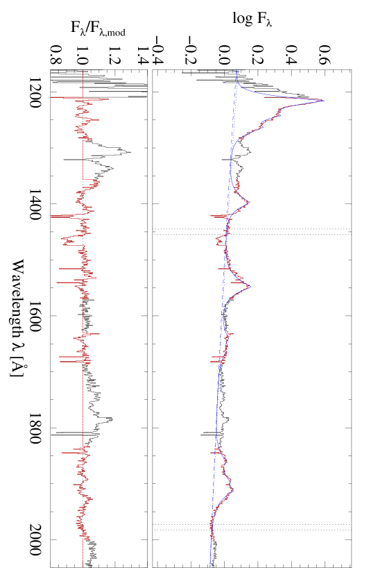
Figure 31: Same as Figure 1 but for the individual spectrum of SDSS J085417.6+532735 ($z=2.42$, $M_{B}=-28.6$), not for quasar composite spectrum.

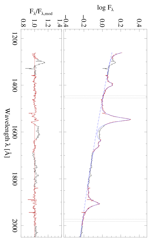
Figure 32: Same as Figure 31 but for SDSS J080342.0+302254 ($z=2.03$, $M_{B}=-28.9$).

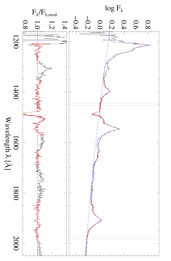
Figure 33: Same as Figure 31 but for SDSS J154359.4+535903 ($z=2.37$, $M_{B}=-28.5$).

However, since the power-law formula is not a conventional one to describe the BLR emission-line profiles, we should be careful to judge whether the power-law formula is a really representative for the BLR emission. In order to investigate whether the power-law emission-line profiles of our quasar composite spectra are due to some artificial effect, rather than resulting from the intrinsic kinematic properties of the BLR, some individual spectra of SDSS quasars with a high S/N are also fitted by using the power-law formula in the same way as for the composite spectra. The fitting results are shown in Figures 31 – 33, where SDSS J085417.6+532735 ($z=2.42$, $M_{B}=-28.6$), SDSS J080342.0+302254 ($z=2.03$, $M_{B}=-28.9$), and SDSS J154359.4+535903 ($z=2.37$, $M_{B}=-28.5$) are investigated. It is clear that the power-law formula describes properly individual spectra of quasars, and not only quasar composite spectra. This suggests that the power-law profile is really representative of the BLR emission and it should be insightful to investigate kinematic properties and the geometrical configuration of gas clouds in BLRs. We do not discuss these issues further because these are beyond the scope of this paper.

In §§2.1, it was mentioned that possible uncertainties in the redshift assigned to each object may introduce artifacts in the emission-line profiles of composite spectra. To check how much this effect might be significant, we investigate the difference in redshift determined by a specific emission line and the redshift assigned for each object by the SDSS pipeline (i.e., the average of various spectral features). What really matters is not the absolute redshift difference between a specific line and the average redshift from other line, but the dispersion of such a difference. As for the Civ$\lambda$1549 emission of quasars with $-26.5>M_{B}\geq-27.5$ at $2.0\leq z<2.5$, the average difference $z_{\rm CIV}-z_{\rm QSO}$ and its standard deviation are $<\!\!z_{\rm CIV}-z_{\rm QSO}\!\!>=-0.007\pm 0.006$. This standard deviation ($\sigma_{<\!\!z_{\rm CIV}-z_{\rm QSO}\!\!>}=0.006$) corresponds to a velocity dispersion of $\sim 1800$ km s^-1. Therefore we should be aware that velocity structures on scales less than this velocity interval of the Civ$\lambda$1549 emission-line profile in the composite spectra may be affected by some artificial effects; more global velocity structures are thought to be free from such effects.

As mentioned in §§2.2, there is another measurement method which has often been adopted, that is the local-continuum method. It is useful to compare the results of our measurements with the values measured by adopting local continuum levels, as in Vanden Berk et al. (2001). In Figure 34, we show the estimated local continuum levels for the wavelength regions around Nv$\lambda$1240, Civ$\lambda$1549 and Ciii]$\lambda$1909. Here we adopt roughly the same $\lambda_{\rm lo}$ and $\lambda_{\rm hi}$ as those defined by Vanden Berk et al. (2001). The local continuum is linear for the wavelength region around Civ$\lambda$1549, while for the wavelength regions around Nv$\lambda$1240 and Ciii]$\lambda$1909 the local continua are determined by third polynomial fitting by using the wavelength parts outside the emission lines. For this comparison, the composite quasar spectrum at $2.0\leq z<2.5$ and $-25.5>M_{B}\geq-26.5$ is used, because most of quasars used by Vanden Berk et al. (2001) are at lower redshift and are less luminous than ours. The flux measurement results are presented in Table 11 and compared with the values of Vanden Berk et al. (2001) and with the results of our method in §§2.2. The fluxes reported by Vanden Berk et al. (2001) are similar to the values measured by us by adopting the local-continuum method, but are very different from the values given in Table 3a obtained by fitting with equation (1). This indicates that the flux measurement for several of the BLR emission lines highly depends on the adopted measurement method. Which method is more appropriate? To tackle this problem, emission-line profiles are very useful, because emission lines with similar ionization potentials are thought to arise in similar regions in BLRs, and therefore should have similar emission-line profiles. In our fitting method, HILs (Nv$\lambda$1240, Civ$\lambda$1549 and Heii$\lambda$1640) have the same velocity profile and the same velocity shift from the systemic velocity by definition. The emission-line width and skewness for each line reported by Vanden Berk et al. (2001) are, on the other hand, very different among these three emission lines; the reported width and skewness are ($\sigma$, Skew) = (2.71${\rm\AA}$, $-0.21$), (14.33${\rm\AA}$, $-0.04$) and (4.43${\rm\AA}$, $-0.22$) for Nv$\lambda$1240, Civ$\lambda$1549 and Heii$\lambda$1640, respectively. The difference of the line skewness should correspond to the difference in the kinematic status of the line-emitting clouds, implying a strong segregation of the line emitting regions among HILs. These line widths correspond to the velocity widths of 655 km s^-1, 2779 km s^-1 and 810 km s^-1, respectively. The difference of a factor of 3–4 in the velocity width corresponds to the difference of a factor of $\sim$10 in the radius from the nucleus, if the BLR motions are dominated by the gravitational potential of the SMBH. As presented in Figure 28, the photoionization model suggests that the emitting region of Nv$\lambda$1240 and Civ$\lambda$1549 are not segregated with a factor of 10 in radius from the nucleus. Reverberation mapping observations also suggest that HILs arise from a similar region, and actually Heii$\lambda$1640 sometimes shows even more rapid time variations than Civ$\lambda$1549 (e.g., Clavel et al. 1991; Korista et al. 1995; Peterson & Wandel 1999). Taking all of the above matters into account, we conclude that our measurement method is better than the local continuum method to measure the emission-line fluxes accurately.

4.2 Comparison of observed line ratios and trends with models

Our analysis on the SDSS DR2 composite spectra clearly indicates that some emission-line flux ratios (Nv/Civ, Siii/Civ, (Siiv+Oiv)/Civ, Aliii/Civ and Nv/Heii) positively correlate with absolute $B$ magnitude with a high statistical significance, but are independent of redshift. As presented in §§3.2, photoionization models suggest that these flux ratios positively correlate with the gas metallicity. This means that the dependences of emission line ratios on absolute $B$ magnitude are caused by the dependence of the BLR gas metallicity on the luminosity. In other words, the BLR gas metallicity positively depends on the quasar luminosity, but independent of the quasar redshift. This conclusion is also suggested by some earlier studies. As for Seyfert 1 galaxies at the local universe, the Ciii]/Civ flux ratio depends strongly on the luminosity (Véron-Cetty et al. 1983), which suggests the dependence of the gas metallicity on the luminosity. The correlation of the BLR metallciity with the quasar luminosity has been reported by, e.g., Hamann & Ferland (1999), Warner et al. (2004), and Shemmer et al. (2004). Warner et al. (2004) also reported the correlation of the BLR metallciity with the mass of SMBHs (see also Shemmer et al. 2004).

The dependence of the gas metallicity on the quasar luminosity is expected, since (1) the quasar luminosity should positively correlate with the mass of SMBHs for a given Eddington accretion ratio, (2) a good correlation between mass of SMBHs and mass of the host galaxies, exists at least in the local universe (e.g., Gebhardt et al. 2000; Ferrarese & Merritt 2000; Marconi & Hunt 2003), and (3) more massive galaxies tend to have higher metallicity gas and stars due to their deeper gravitational potential (e.g., Pagel & Edmunds 1981; Arimoto & Yoshii 1987; Matteucci & Tornambè 1987; Tremonti et al. 2004). The results presented in this paper indicate the existence of close relation between mass of SMBHs and host galaxies, and that the galaxy mass-metallicity relation holds also at high redshift, up to $z\sim 4.5$. We should mention that the independence of broad emission-line flux ratios from redshift may be due to some selection effects. For instance, quasars with low metallicity may be dust-enshrouded in their young phase and thus very difficult to detect (see, e.g., Kawakatu et al. 2003). Hard X-ray deep and wide surveys are required to examine this possibility.

However, by comparing the measured flux ratios with the results of the photoionization model calculations with fixed weighting functions ($\beta$ and $\Gamma$ in §3), the inferred gas metallicity is apparently different depending on the adopted flux ratio. For instance, the observed ratios of Nv/Civ, (Siiv+Oiv)/Civ, Aliii/Civ and Nv/Heii suggest gas metallicities of $Z/Z_{\odot}>2$, while the ratios of Cii/Civ, (Oiii]+Alii)/Civ, Siiii]/Civ and Ciii]/Civ suggest $Z/Z_{\odot}\la 2$ (Figure 29). The ratio of Heii/Civ is also not reproduced in most cases. This is consistent with earlier works that the estimates of the BLR metallicity using only the Nv/Civ and/or Nv/Heii flux ratios alone might be quite uncertain (see Hamann et al. 2002). As for the ratio of Siii/Civ, the observed value deviates completely from the range of model predictions. The deviation of Siii/Civ may be due to the contamination of other emission lines into the Siii. Indeed, we find that the flux of Sii$\lambda$1256 becomes high under some physical conditions. In Figure 35, we show the predicted flux ratio of Sii/Siii for $Z/Z_{\odot}$ = 1.0 and 5.0, and $U=10^{-2.5}$ and $10^{-3.5}$ as a function of gas metallicity, adopting the ionizing continuum SED with a large UV thermal bump. The Sii/Siii ratio exceeds 0.2 and reaches $\sim$1 for models with high gas densities. Apparently the contribution of the Sii flux makes the deviation of the measured Siii/Civ ratio from the theoretically predicted range. Apart from the Siii deviation issue, what causes the discrepancies among the inferred metallicity from different line ratios? SED effects are an implausible explanation of this problem, because we have already seen in Figure 29 that the predicted line flux ratios do not vary so significantly by changing the adopted SED. Since the SEDs adopted in this paper (Figure 27) are thought to be extreme, opposite cases for the actual ionizing continuum of quasars, the SED effects on the flux ratios should be smaller than those presented in Figure 29.

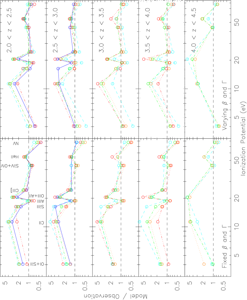
Figure 37: Ratios of predicted to observed emission-line fluxes normalized to the Civ flux, as a function of the ionization potential of corresponding ions. Model predictions with fixed $\beta$ and $\Gamma$ and those with varying $\beta$ and $\Gamma$ are presented in the left and right panels, respectively. Results for composite spectra of $2.0\leq z<2.5$, $2.5\leq z<3.0$, $3.0\leq z<3.5$, $3.5\leq z<4.0$ and $4.0\leq z<4.5$ quasars are shown at upper to lower panels. Results for composite spectra of $-24.5>M_{B}\geq-25.5$, $-25.5>M_{B}\geq-26.5$, $-26.5>M_{B}\geq-27.5$, $-27.5>M_{B}\geq-28.5$ and $-28.5>M_{B}\geq-29.5$ are denoted by solid blue lines, dashed light-blue lines, dash-dotted green lines, dotted orange lines, and dash-dot-dot-dotted red lines, respectively. Dashed horizontal lines denote the unity of ratios of predicted to observed fluxes. For ionization parameters of emission-line pairs, the average values are adopted just for the presentation; i.e., 4.05 eV for Oi+Siii, 20.5 eV for Oiii+Alii, and 44.2 eV for Siiv+Oiv.

One possibility which can cause the discrepancies of the inferred metallicities from various emission-line flux ratios is that the assumption on the weighting functions $\Gamma$ and $\beta$ is an oversimplification. To examine this possibility quantitatively, we investigate the dependence of the theoretical predictions of some emission-line flux ratios on the adopted $\Gamma$ and $\beta$ parameters, as shown in Figure 36. It is clear that various predicted emission-line flux ratios are highly dependent on the adopted values of $\Gamma$ and $\beta$. Since the theoretical flux ratios presented in Figure 29 are predicted by adopting $\Gamma=-1$ and $\beta=-1$ (as in many other studies), other assumptions on $\beta$ and $\Gamma$ result in other predictions and thus the metallicity inferred by each one of the observed emission-line flux ratios would change accordingly. In order to derive a more accurate metallicity for each composite spectrum, a better approach is to vary the indices of $\Gamma$ and $\beta$ to fit as many as emission lines as possible through the model predictions with a certain metallicity. Therefore we performed a fit of all available flux ratios for each composite spectrum by varying gas metallicity, SED, $\Gamma$ and $\beta$. We first associated errors on the line fluxes with the following recipe: (i) we set the minimum relative error to 5% and (ii) in any case, absolute errors cannot be less than 1% of the absolute flux of Civ$\lambda$1549. The best fit $\beta$ and $\Gamma$ are obtained by minimizing $\chi^{2}$ computed using the logarithm of model and observed line fluxes. This allows us to give more weight to the points where the ratio between model and observed values is smaller. We then perform the optimization on $\beta$ and $\Gamma$ for each spectral composite, using all continua and abundance sets. In Tables 12–16 we show, for each spectral composite, the model with the lowest $\chi^{2}$ and the corresponding abundances set, as well as the $\beta$ and $\Gamma$ values. For comparison, we also show the best models with the classical $\beta=-1$ and $\Gamma=-1$. The models with optimized $\beta$ and $\Gamma$ provide a much better description of the observed data but in most cases the inferred metallicities are similar: $Z/Z_{\odot}=5.0$ for most cases, and $Z/Z_{\odot}=2.0$ or 10.0 for some other cases. In a few cases the metallicity obtained by varying $\beta$ and $\Gamma$ are lower than inferred by the models with fixed $\beta=-1$ and $\Gamma=-1$. Our results may be partly affected by the lack of the resolution of metallicity in our model calculation, but they suggest that the typical metallicity of the gas in the BLRs is $\sim 5Z_{\odot}$, or at least a super-solar value. In all cases the optimized $\beta$ values are lower, but close to, –1. $\Gamma$ is generally in the range $-2.0<\Gamma<-1.5$, and always $\Gamma<-1$. It is interesting that the dispersions of the best-fit $\beta$ and $\Gamma$ is very small. The averaged values are $\beta=-1.08$ and $\Gamma=-1.52$, and their RMS’s are 0.05 and 0.13, respectively. This result suggests that the commonly adopted values of $\beta=-1$ and $\Gamma=-1$ are not the best choice. The best-fit values of $\beta$ and $\Gamma$ may imply some specific physical properties for the BLR, although we do not discuss this issue further in this paper. Best-fit models and observations are compared graphically in Figure 37. Niv]/Civ is not shown because its weighting factor in the fitting process is very low (the errors are very large with respect to the Niv]/Civ flux ratios; Table 12–16) and thus the fitting results are nearly meaningless for this flux ratio. For the same reason, the results for Cii/Civ are not good. Apart from these two flux ratios, the fitting results appear in better agreement with the observations when allowing $\beta$ and $\Gamma$ to be free. Interestingly, large Nv/Civ ratios can be rather easily explained when the weighting functions are varied. This suggests that the BLR metallicity cannot be determined uniquely by using just Nv/Civ (or Nv/Heii).

In order to illustrate our results on the metallicity trends in a graphical way, for the reader’s convenience, Figure 38 shows the metallicity, averaged in luminosity, as a function of redshift. Here we use the metallicities derived by the fit with varying $\beta$ and $\Gamma$ given in Tables 12–16. To avoid biases when calculating the average metallicity, we have only used the luminosity bins for which a metallicity determination is available at all redshifts. This limits the range of usable luminosities to $-25.5>M_{B}>-28.5$, where the averaged metallicity are calculated. The errorbars are the estimated errors on the mean obtained by combining the uncertainty in the metallicity determination for each luminosity bin. The resulting plot shows what was already clear from Tables 12–16 and from our earlier discussion, i.e., there is no significant evolution of the metallicity as a function of redshift. Figure 39 shows the complementary diagram, i.e., the metallicity, averaged in redshift, as a function of luminosity. Again, to avoid biases when calculating the averaged metallicity, we have only used the redshift bins for which a metallicity determination is available at all luminosities, which limits the range of usable redshifts to $2<z<3$. The resulting diagram shows that the averaged metallicity increases significantly with absolute magnitude, as already inferred from the individual results in Tables 12–16.

Another possibility which may cause the discrepancies among the gas metallicities inferred from each emission-line flux ratio is the elemental abundance ratios. In our model, the relative elemental abundances are assumed to scale proportionally to solar, except for nitrogen which is assumed to scale as the square of other metal abundances. However these assumptions are an oversimplification. In more realistic metallicity evolutionary scenarios abundances never scale linearly with the global metallicity (e.g., Pipino & Matteucci 2004). The inclusion of more realistic abundance pattern in our photoionization models will be presented in a forthcoming paper.

Our analysis on the composite spectra shows that there is no apparent dependence of emission-line flux ratios on redshift up to $z\sim 4.5$, which is consistent with the results of Dietrich et al. (2002). This suggests that the chemical composition of the gas clouds in BLRs does not change significantly up to $z\sim 4.5$. Although the $\alpha$ elements, such as oxygen, can be enriched on a very short timescale ($\ll$ 1 Gyr) owing to type II supernovae, the enrichment of carbon and silicon require longer timescales ($\sim$0.5–1 Gyr) since they are produced mainly by the low-mass or intermediate-mass evolved stars. Therefore, if the elemental abundance ratios in BLRs remain constant up to high redshift, this gives a strong constraint on the first epoch of active star-formation in quasar host galaxies. In particular, constant elemental abundance ratios up to $z=4.5$ suggest that the main star-formation epoch in the host galaxies occurred at $z\ga 7$, when minimum timescale to enrich C and Si is taken into account. However this kind of discussion requires a detailed theoretical predictions of the metal enrichment history based on galaxy chemical evolutionary models. Theoretical studies on the BLR evolution coupled with galaxy evolutionary models are thus crucial to understand the quasar formation and evolution. Here we mention that possible variations of the emission-line spectra beyond $z=4$ might be present in Figure 23, though the statistical significance is not high enough. Further spectroscopic observations of quasars in this redshift range or even at higher redshifts, for sizeable samples of quasars, would be highly insightful to examine the quasar evolutionary scenarios.

Similarly to some emission-line flux ratios, the velocity shift of HILs relative to LILs also correlates with the quasar luminosity and is independent of quasar redshift, as presented in Figure 26. The velocity difference between HILs and LILs has been analyzed for a long time to investigate various kinematic/geometrical models for BLRs (e.g., Gaskell 1982; Wilkes 1984, 1986; Espey et al. 1989; Corbin 1990; Vanden Berk et al. 2001). The correlation between this velocity difference and the quasar luminosity has been reported also by other studies (e.g., Corbin 1990; Richards et al. 2002b). Our results confirm those previous works and reveal their independence of redshift.

Finally we discuss the nature of the ”1600${\rm\AA}$ bump”. This unidentified emission feature has been noted in earlier studies, e.g., Wilkes (1984) and Boyle (1990). Our analysis on the composite spectra clarifies that the 1600${\rm\AA}$ bump is universally seen in spectra of quasars. Laor et al. (1994) clearly presented this emission feature in some low-redshift quasars. The 1600${\rm\AA}$ bump of the sample of Laor et al. (1994) is characterized by FWHM $\sim$ 12000–24000 km s^-1 and $\Delta v_{1600}\sim 1700-8200$ km s^-1 if it is one of Civ$\lambda$1549 components. They also found a very redshifted broad component for Ly$\alpha$ and Ovi$\lambda$1034 (see Table 4 of Laor et al. 1994), which appears to support the interpretation that the 1600${\rm\AA}$ bump is one of Civ$\lambda$1549 components. If this is the case, a slight negative correlation between the flux ratio of the 1600${\rm\AA}$ bump to Civ$\lambda$1549 and the quasar luminosity (Figure 25) may be due to some luminosity dependence of the structure of the Civ$\lambda$1549-emitting region in the BLR. The 1600${\rm\AA}$ bump may be, otherwise, a blueshifted component of the Heii$\lambda$1640 emission. This interpretation is inferred by the negative correlation of the flux ratio of the 1600${\rm\AA}$ bump to Civ$\lambda$1549 with the quasar luminosity, because the Heii/Civ ratio also shows the similar negative correlation with the quasar luminosity (Figure 25). However similar blueshifted spectral profile should appear for the emission lines with a similar ionization degree such as Civ$\lambda$1549, which is not the case for our composite quasar spectra. One possibility might be the presence of outflowing very dense gas clouds with a low ionization parameter. As shown in Figure 28, gas clouds with low $\Phi$ and high $n$ radiate Heii$\lambda$1640 emission, but do not radiate the Civ$\lambda$1549 emission. This idea could be tested by examining velocity profiles of the other transition of Heii. Although the Heii Fowler lines ($\lambda$4686, $\lambda$3203, …) may be difficult to investigate due to their blending with the strong Feii multiplet emission, the Heii Pickering lines, especially Heii$\lambda$10124 may be useful to perform this test. Alternatively, the 1600${\rm\AA}$ bump may be caused by the UV Feii multiplet emission. Sometimes at $\sim 1600{\rm\AA}$, the Feii feature is seen in emission in quasars (e.g., Marziani et al. 1996; Vestergaard & Wilkes 2001; Vestergaard & Peterson 2005) or in absorption in low-ionization BALs (e.g., Hall et al. 2002). As for the sample of Laor et al. (1994), the quasars with a stronger UV Feii multiplet emission appear to show also stronger 1600${\rm\AA}$ bump, which may support the interpretation that the 1600${\rm\AA}$ bump is also a part of the UV Feii multiplet emission. The only problem with the Feii scenario is the interpretation of the anti-correlation of (1600${\rm\AA}$ bump)/Civ with luminosity, which is not seen in other low-ionization lines.

5 Summary

In order to investigate the properties of BLR gas clouds as a function of quasar luminosity and redshift, we made composite spectra of the SDSS DR2 quasars in the ranges of $2.0\leq z\leq 4.5$ and $-24.5\geq M_{B}\geq-29.5$ for each luminosity and redshift bin with $\Delta M_{B}=1.0$ mag and $\Delta z=0.5$. By analyzing these composite spectra, we obtained the following results.

• The emission lines in the composite spectra are better fitted with power-law profiles than with double Gaussian or modified Lorentzian profiles. Such power-law profile fitting method appears also to be more appropriate to measure broad emission-line fluxes than the method of using a local continuum level for each emission lines and then directly integrating the line flux.

• The flux ratios of Nv/Civ, (Siiv+Oiv)/Civ, Aliii/Civ, Siiii]/Civ and Nv/Heii show statistically significant positive correlations with absolute $B$ magnitude.

• Most of the examined flux ratios show no statistically significant correlation with redshift.

• Recession velocity differences between HILs and LILs, as well as emission-line widths, also show strong correlations with the quasar luminosity, while being independent of redshift.

To interpret these findings, we performed extensive photoionization model calculations. By comparing the results of our calculations with the observational data, we obtained the following results.

• A natural interpretation of the dependence of the flux ratios on quasar luminosity is that more luminous quasars are characterized by more metal-rich gas in their BLR.

• The typical metallicity of the gas in BLRs is estimated to be $\sim 5Z_{\odot}$, or at least super-solar.

The absence of a significant metallicity variation up to $z\sim 4.5$ implies that the active star-formation epoch of quasar host galaxies occurred at $z\ga 7$. To examine this issue further, observations of rest-frame UV spectra of quasars at $z\ga 4.5$ through near-infrared spectroscopy are crucially necessary.

Figure 12: Same as Figure 1 but for the composite spectrum of quasars with $-26.5>M_{B}\geq-27.5$ and $3.0\leq z<3.5$.

Figure 22: Measured flux ratios as a function of redshift. Open circles, squares, triangles, pluses, and stars denote the composite spectra for $-24.5>M_{B}\geq-25.5$, $-25.5>M_{B}\geq-26.5$, $-26.5>M_{B}\geq-27.5$, $-27.5>M_{B}\geq-28.5$, and $-28.5>M_{B}\geq-29.5$, respectively.

Figure 23: Measured flux ratios as a function of absolute $B$ magnitude. Open circles, squares, triangles, pluses, and stars denote the composite spectra for $2.0\leq z<2.5$, $2.5\leq z<3.0$, $3.0\leq z<3.5$, $3.5\leq z<4.0$, and $4.0\leq z<4.5$, respectively.

Figure 24: Flux ratios normalized by the value measured on composite spectra at $2.0\leq z<2.5$ for the individual luminosity bins, as a function of redshift. Symbols are the same as those in Figure 22. Results of the linear fitting are shown by dotted lines.

Figure 25: Flux ratios normalized by the value measured on composite spectra at $-26.5>M_{B}\geq-27.5$ for the individual redshift bins, as a function of absolute $B$ magnitude. Symbols are the same as those in Figure 23. Results of the linear fitting are shown by dotted lines.

Figure 26: Velocity shift of high-ionization lines (HILs) in relative to that of low-ionization lines (LILs) (upper panels), FWHM of HILs (middle panels) and LILs (lower panels), as functions of redshift (left panels) and absolute $B$ magnitude (right panels). In the left panel, open circles, squares, triangles, pluses, and stars denote the data for $-24.5>M_{B}\geq-25.5$, $-25.5>M_{B}\geq-26.5$, $-26.5>M_{B}\geq-27.5$, $-27.5>M_{B}\geq-28.5$, and $-28.5>M_{B}\geq-29.5$, respectively. In the right panel, open circles, squares, triangles, pluses, and stars denote the data for $2.0\leq z<2.5$, $2.5\leq z<3.0$, $3.0\leq z<3.5$, $3.5\leq z<4.0$, and $4.0\leq z<4.5$, respectively.

Figure 27: Adopted SEDs for our photoionization model calculations. Thin solid line denotes a SED with a strong UV bump and thick dashed line denotes a SED with a weak UV bump. These SEDs are normalized to the flux at 1 keV ($\simeq$73 Ryd).

Figure 28: Results of model calculations for H$\beta$ $\lambda$4861, Heii$\lambda$1640, Ciii]$\lambda$1909, Civ$\lambda$1640, Nv$\lambda$1240 and Aliii$\lambda$1857. The equivalent widths referenced to the incident continuum at 1215${\rm\AA}$ are displayed as contours. The smallest decade contour corresponds to 1${\rm\AA}$, and the contour step size is 0.2 dex in logscale. Only models with an input SED with a large UV thermal bump and a metallicity of $Z/Z_{\odot}=1.0$ are shown as examples.

Figure 29: Theoretical emission-line flux ratios calculated by the LOC photoionization model, as a function of gas metallicity. Solid and dashed lines denote the models with a large and a small UV thermal bump. For blended lines, in addition to the individual emission lines, their total flux are drawn with thick lines.

Figure 30: Spectral fitting by adopting equation (1) ($left$), double Gaussian ($middle$) and modified Lorentzian ($right$), for emission lines. The composite spectrum and the model fit are shown in upper panels while the residual spectrum is shown in lower panels. The presented composite spectrum is for quasars at $2.0\leq z<2.5$ and $-26.5>M_{B}\geq-27.5$.

Figure 34: Examples of the estimated local continuum (dotted lines) for a few lines. The composite spectrum used here is for quasars at $2.0\leq z<2.5$ and $-26.5>M_{B}\geq-27.5$.

Figure 35: Predicted Sii$\lambda$1257/Siii$\lambda$1263 flux ratio as a function of gas density. Solid, dashed, dot-dashed and dotted lines denote the models with ($Z/Z_{\odot}$, log $U$) = (1.0, –2.5), (1.0, –3.5), (5.0, –2.5), and (5.0, –3.5), respectively.

Figure 36: Integrated theoretical flux ratios as a function of $\Gamma$ ($left$) and $\beta$ ($right$). Only the models with $Z/Z_{\odot}$ = 1.0 and with a small UV bump SED are shown. Predicted flux ratios of Nv/Civ, Heii/Civ, Aliii/Civ, Siiii]/Civ and Ciii]/Civ are denoted by solid, dotted, dashed, dot-dashed, and three-dot-dashed lines, respectively.

Figure 38: Estimated metallicities from our composite spectra, averaged in the luminosity range $-25.5>M_{B}>-28.5$, as a function of redshift. The estimation of the metallicity given in this figure is derived from the fit with the varying $\beta$ and $\Gamma$, which are presented in Tables 12–16.

Figure 39: Estimated metallicities from our composite spectra, averaged in the redshift range $2.0\leq z<3.0$, as a function of luminosity. The estimation of the metallicity given in this figure is derived from the fit with the varying $\beta$ and $\Gamma$, which are presented in Tables 12 and 13.

Table 1: Number distribution of our quasar sample among the redshift and the absolute magnitude bins

	$2.0\leq z<2.5$	$2.5\leq z<3.0$	$3.0\leq z<3.5$	$3.5\leq z<4.0$	$4.0\leq z<4.5$	total
$-24.5>M_{B}\geq-25.5$	643	50	1	0	0	694
$-25.5>M_{B}\geq-26.5$	1497	284	332	153	25	2291
$-26.5>M_{B}\geq-27.5$	917	385	323	222	120	1967
$-27.5>M_{B}\geq-28.5$	105	71	76	53	45	350
$-28.5>M_{B}\geq-29.5$	5	11	16	5	3	40
$-29.5>M_{B}\geq-30.5$	0	1	1	0	0	2
total	3167	802	749	433	193	5344

Table 2: Ionization potentials of ions

Ion	Ionization Potential	Ionization Potential	Classification
	Lower (eV)	Upper (eV)
Oi	0.0	13.6	LIL
Alii	5.9	18.8	LIL
Siii	8.1	16.3	LIL
Cii	11.3	24.4	LIL
Siiii	16.3	33.5	LIL
Aliii	18.8	28.4	LIL
Ciii	24.4	47.9	LIL
Heii	24.6	54.4	HILa
Siiv	33.5	45.1	LIL
Oiii	35.1	54.9	LIL
Niv	47.4	77.4	HIL
Civ	47.9	64.5	HIL
Oiv	54.9	77.4	HIL
Nv	77.4	97.9	HIL

• Classified as a HIL because Heii$\lambda$1640 is a recombination line and thus the $upper$ ionization potential is important rather than the $lower$ ionization potential.

Table 3: Measured line fluxes; $2.0\leq z<2.5$

Line	$-24.5\!>\!M_{B}\!\geq\!-25.5$	$-25.5\!>\!M_{B}\!\geq\!-26.5$	$-26.5\!>\!M_{B}\!\geq\!-27.5$	$-27.5\!>\!M_{B}\!\geq\!-28.5$	$-28.5\!>\!M_{B}\!\geq\!-29.5$
Nv$\lambda$1240	0.506 $\pm$ 0.004	0.717 $\pm$ 0.007	0.887 $\pm$ 0.010	0.983 $\pm$ 0.012	1.144 $\pm$ 0.016
Siii$\lambda$1263	0.089 $\pm$ 0.001	0.126 $\pm$ 0.002	0.140 $\pm$ 0.002	0.176 $\pm$ 0.003	0.222 $\pm$ 0.003
Oi $\!\!+\!\!$ Siii$\lambda$1305	0.061 $\pm$ 0.002	0.081 $\pm$ 0.002	0.086 $\pm$ 0.002	0.085 $\pm$ 0.002	0.145 $\pm$ 0.004
Cii$\lambda$1335	0.033 $\pm$ 0.002	0.047 $\pm$ 0.001	0.052 $\pm$ 0.001	0.050 $\pm$ 0.002	0.089 $\pm$ 0.004
Siiv$\lambda$1397	0.111 $\pm$ 0.002	0.027 $\pm$ 0.003	0.001 $\pm$ 0.016	0.033 $\pm$ 0.003	—
Oiv]$\lambda$1402	0.145 $\pm$ 0.008	0.308 $\pm$ 0.008	0.374 $\pm$ 0.019	0.365 $\pm$ 0.010	0.419 $\pm$ 0.008
Niv]$\lambda$1486	0.017 $\pm$ 0.000	0.013 $\pm$ 0.000	0.015 $\pm$ 0.000	0.020 $\pm$ 0.000	—
Civ$\lambda$1549	1.000 $\pm$ 0.007	1.000 $\pm$ 0.008	1.000 $\pm$ 0.010	1.000 $\pm$ 0.010	1.000 $\pm$ 0.012
1600Å bump	0.112 $\pm$ 0.002	0.106 $\pm$ 0.002	0.098 $\pm$ 0.002	0.097 $\pm$ 0.003	0.060 $\pm$ 0.005
Heii$\lambda$1640	0.147 $\pm$ 0.001	0.152 $\pm$ 0.001	0.149 $\pm$ 0.002	0.140 $\pm$ 0.001	0.133 $\pm$ 0.002
Oiii]$\lambda$1663	0.077 $\pm$ 0.001	0.083 $\pm$ 0.002	0.072 $\pm$ 0.002	0.083 $\pm$ 0.003	0.104 $\pm$ 0.002
Alii$\lambda$1671	0.010 $\pm$ 0.001	0.010 $\pm$ 0.001	0.022 $\pm$ 0.001	0.018 $\pm$ 0.001	—
Aliii$\lambda$1857	0.064 $\pm$ 0.001	0.092 $\pm$ 0.001	0.105 $\pm$ 0.001	0.124 $\pm$ 0.002	0.146 $\pm$ 0.002
Siiii]$\lambda$1892	0.093 $\pm$ 0.001	0.118 $\pm$ 0.001	0.127 $\pm$ 0.001	0.129 $\pm$ 0.002	0.110 $\pm$ 0.002
Ciii]$\lambda$1909	0.285 $\pm$ 0.005	0.326 $\pm$ 0.008	0.326 $\pm$ 0.008	0.348 $\pm$ 0.010	0.395 $\pm$ 0.012

Table 4: Measured line fluxes; $2.5\leq z<3.0$

Line	$-24.5\!>\!M_{B}\!\geq\!-25.5$	$-25.5\!>\!M_{B}\!\geq\!-26.5$	$-26.5\!>\!M_{B}\!\geq\!-27.5$	$-27.5\!>\!M_{B}\!\geq\!-28.5$	$-28.5\!>\!M_{B}\!\geq\!-29.5$
Nv$\lambda$1240	0.561 $\pm$ 0.004	0.578 $\pm$ 0.005	0.858 $\pm$ 0.010	1.004 $\pm$ 0.013	1.248 $\pm$ 0.018
Siii$\lambda$1263	0.160 $\pm$ 0.001	0.117 $\pm$ 0.001	0.149 $\pm$ 0.002	0.194 $\pm$ 0.003	0.210 $\pm$ 0.003
Oi $\!\!+\!\!$ Siii$\lambda$1305	0.121 $\pm$ 0.006	0.089 $\pm$ 0.002	0.095 $\pm$ 0.002	0.119 $\pm$ 0.002	0.112 $\pm$ 0.005
Cii$\lambda$1335	0.065 $\pm$ 0.006	0.037 $\pm$ 0.002	0.055 $\pm$ 0.002	0.059 $\pm$ 0.002	0.074 $\pm$ 0.004
Siiv$\lambda$1397	0.052 $\pm$ 0.002	0.160 $\pm$ 0.002	—	—	—
Oiv]$\lambda$1402	0.202 $\pm$ 0.003	0.092 $\pm$ 0.002	0.360 $\pm$ 0.008	0.401 $\pm$ 0.007	0.462 $\pm$ 0.027
Niv]$\lambda$1486	0.021 $\pm$ 0.000	0.029 $\pm$ 0.000	0.022 $\pm$ 0.000	0.019 $\pm$ 0.000	0.012 $\pm$ 0.001
Civ$\lambda$1549	1.000 $\pm$ 0.006	1.000 $\pm$ 0.007	1.000 $\pm$ 0.010	1.000 $\pm$ 0.011	1.000 $\pm$ 0.012
1600Å bump	0.125 $\pm$ 0.008	0.111 $\pm$ 0.003	0.103 $\pm$ 0.002	0.092 $\pm$ 0.003	0.100 $\pm$ 0.006
Heii$\lambda$1640	0.151 $\pm$ 0.001	0.146 $\pm$ 0.001	0.151 $\pm$ 0.002	0.143 $\pm$ 0.002	0.125 $\pm$ 0.002
Oiii]$\lambda$1663	0.087 $\pm$ 0.001	0.083 $\pm$ 0.002	0.093 $\pm$ 0.003	0.086 $\pm$ 0.003	0.096 $\pm$ 0.002
Alii$\lambda$1671	—	0.015 $\pm$ 0.001	0.013 $\pm$ 0.001	0.017 $\pm$ 0.001	—
Aliii$\lambda$1857	0.078 $\pm$ 0.001	0.071 $\pm$ 0.001	0.102 $\pm$ 0.001	0.109 $\pm$ 0.002	0.165 $\pm$ 0.003
Siiii]$\lambda$1892	0.070 $\pm$ 0.001	0.063 $\pm$ 0.001	0.108 $\pm$ 0.001	0.152 $\pm$ 0.002	0.204 $\pm$ 0.003
Ciii]$\lambda$1909	0.375 $\pm$ 0.006	0.351 $\pm$ 0.007	0.354 $\pm$ 0.010	0.328 $\pm$ 0.008	0.331 $\pm$ 0.004

Table 5: Measured line fluxes; $3.0\leq z<3.5$

Line	$-25.5\!>\!M_{B}\!\geq\!-26.5$	$-26.5\!>\!M_{B}\!\geq\!-27.5$	$-27.5\!>\!M_{B}\!\geq\!-28.5$	$-28.5\!>\!M_{B}\!\geq\!-29.5$
Nv$\lambda$1240	0.635 $\pm$ 0.005	0.819 $\pm$ 0.009	1.034 $\pm$ 0.013	0.979 $\pm$ 0.011
Siii$\lambda$1263	0.126 $\pm$ 0.002	0.161 $\pm$ 0.002	0.183 $\pm$ 0.003	0.198 $\pm$ 0.003
Oi $\!\!+\!\!$ Siii$\lambda$1305	0.090 $\pm$ 0.002	0.095 $\pm$ 0.002	0.109 $\pm$ 0.003	0.094 $\pm$ 0.004
Cii$\lambda$1335	0.050 $\pm$ 0.002	0.049 $\pm$ 0.002	0.055 $\pm$ 0.003	0.039 $\pm$ 0.004
Siiv$\lambda$1397	0.102 $\pm$ 0.001	0.043 $\pm$ 0.003	0.075 $\pm$ 0.003	—
Oiv]$\lambda$1402	0.176 $\pm$ 0.004	0.286 $\pm$ 0.007	0.327 $\pm$ 0.005	0.370 $\pm$ 0.006
Niv]$\lambda$1486	0.030 $\pm$ 0.000	0.023 $\pm$ 0.000	0.019 $\pm$ 0.000	0.045 $\pm$ 0.001
Civ$\lambda$1549	1.000 $\pm$ 0.007	1.000 $\pm$ 0.010	1.000 $\pm$ 0.011	1.000 $\pm$ 0.010
1600Å bump	0.117 $\pm$ 0.003	0.117 $\pm$ 0.003	0.099 $\pm$ 0.004	0.083 $\pm$ 0.005
Heii$\lambda$1640	0.148 $\pm$ 0.001	0.148 $\pm$ 0.001	0.148 $\pm$ 0.002	0.102 $\pm$ 0.001
Oiii]$\lambda$1663	0.084 $\pm$ 0.002	0.092 $\pm$ 0.002	0.078 $\pm$ 0.003	0.088 $\pm$ 0.003
Alii$\lambda$1671	0.027 $\pm$ 0.001	0.019 $\pm$ 0.001	0.030 $\pm$ 0.001	0.012 $\pm$ 0.001
Aliii$\lambda$1857	0.072 $\pm$ 0.001	0.109 $\pm$ 0.001	0.126 $\pm$ 0.002	0.117 $\pm$ 0.001
Siiii]$\lambda$1892	0.068 $\pm$ 0.001	0.112 $\pm$ 0.001	0.105 $\pm$ 0.001	0.134 $\pm$ 0.001
Ciii]$\lambda$1909	0.337 $\pm$ 0.007	0.321 $\pm$ 0.007	0.379 $\pm$ 0.010	0.281 $\pm$ 0.007

Table 6: Measured line fluxes; $3.5\leq z<4.0$

Line	$-25.5\!>\!M_{B}\!\geq\!-26.5$	$-26.5\!>\!M_{B}\!\geq\!-27.5$	$-27.5\!>\!M_{B}\!\geq\!-28.5$	$-28.5\!>\!M_{B}\!\geq\!-29.5$
Nv$\lambda$1240	0.617 $\pm$ 0.005	0.856 $\pm$ 0.010	1.062 $\pm$ 0.012	1.001 $\pm$ 0.015
Siii$\lambda$1263	0.129 $\pm$ 0.001	0.156 $\pm$ 0.002	0.194 $\pm$ 0.002	0.083 $\pm$ 0.001
Oi $\!\!+\!\!$ Siii$\lambda$1305	0.098 $\pm$ 0.006	0.105 $\pm$ 0.004	0.115 $\pm$ 0.005	0.180 $\pm$ 0.013
Cii$\lambda$1335	0.030 $\pm$ 0.006	0.051 $\pm$ 0.004	0.062 $\pm$ 0.005	0.105 $\pm$ 0.013
Siiv$\lambda$1397	0.196 $\pm$ 0.002	—	—	0.024 $\pm$ 0.016
Oiv]$\lambda$1402	0.065 $\pm$ 0.007	0.347 $\pm$ 0.008	0.395 $\pm$ 0.009	0.398 $\pm$ 0.017
Niv]$\lambda$1486	0.038 $\pm$ 0.000	0.025 $\pm$ 0.000	0.016 $\pm$ 0.000	0.031 $\pm$ 0.001
Civ$\lambda$1549	1.000 $\pm$ 0.006	1.000 $\pm$ 0.010	1.000 $\pm$ 0.010	1.000 $\pm$ 0.013
1600Å bump	0.106 $\pm$ 0.008	0.113 $\pm$ 0.005	0.100 $\pm$ 0.007	0.032 $\pm$ 0.016
Heii$\lambda$1640	0.153 $\pm$ 0.001	0.145 $\pm$ 0.002	0.128 $\pm$ 0.001	0.108 $\pm$ 0.001
Oiii]$\lambda$1663	0.081 $\pm$ 0.001	0.083 $\pm$ 0.001	0.089 $\pm$ 0.002	0.056 $\pm$ 0.001
Alii$\lambda$1671	0.016 $\pm$ 0.001	0.017 $\pm$ 0.001	—	—
Aliii$\lambda$1857	0.084 $\pm$ 0.001	0.098 $\pm$ 0.001	0.121 $\pm$ 0.002	0.124 $\pm$ 0.002
Siiii]$\lambda$1892	0.066 $\pm$ 0.001	0.122 $\pm$ 0.001	0.186 $\pm$ 0.002	0.193 $\pm$ 0.003
Ciii]$\lambda$1909	0.355 $\pm$ 0.006	0.332 $\pm$ 0.008	0.343 $\pm$ 0.007	0.426 $\pm$ 0.010

Table 7: Measured line fluxes; $4.0\leq z<4.5$

Line	$-25.5\!>\!M_{B}\!\geq\!-26.5$	$-26.5\!>\!M_{B}\!\geq\!-27.5$	$-27.5\!>\!M_{B}\!\geq\!-28.5$
Nv$\lambda$1240	0.724 $\pm$ 0.004	0.933 $\pm$ 0.010	1.075 $\pm$ 0.013
Siii$\lambda$1263	0.251 $\pm$ 0.003	0.249 $\pm$ 0.004	0.217 $\pm$ 0.005
Oi $\!\!+\!\!$ Siii$\lambda$1305	0.148 $\pm$ 0.012	0.146 $\pm$ 0.005	0.134 $\pm$ 0.005
Cii$\lambda$1335	0.067 $\pm$ 0.012	0.068 $\pm$ 0.005	0.064 $\pm$ 0.005
Siiv$\lambda$1397	0.205 $\pm$ 0.003	0.379 $\pm$ 0.009	0.055 $\pm$ 0.006
Oiv]$\lambda$1402	0.144 $\pm$ 0.007	0.004 $\pm$ 0.015	0.354 $\pm$ 0.010
Niv]$\lambda$1486	0.019 $\pm$ 0.000	0.010 $\pm$ 0.000	0.007 $\pm$ 0.000
Civ$\lambda$1549	1.000 $\pm$ 0.004	1.000 $\pm$ 0.009	1.000 $\pm$ 0.011
1600Å bump	0.075 $\pm$ 0.015	0.070 $\pm$ 0.007	0.061 $\pm$ 0.007
Heii$\lambda$1640	0.132 $\pm$ 0.001	0.095 $\pm$ 0.001	0.095 $\pm$ 0.001
Oiii]$\lambda$1663	0.048 $\pm$ 0.002	0.064 $\pm$ 0.002	0.029 $\pm$ 0.001
Alii$\lambda$1671	0.000 $\pm$ 0.001	—	0.046 $\pm$ 0.001

Table 8: Measured velocity shift and line width of HILs and LILs

Redshift	Magnitude	Line	Velocity Shift	Profile Parameter		FWHMa
			(km/s)	$\alpha$	$\beta$	(km/s)
$2.0\!\leq\!z\!<\!2.5$	$-24.5\!>\!M_{B}\!\geq\!-25.5$	HIL	–464.9 $\pm$ 1.2	117.30 $\pm$ 0.02	99.37 $\pm$ 0.02	3858
		LIL	–83.4 $\pm$ 1.9	114.49 $\pm$ 0.05	119.60 $\pm$ 0.07	3550
	$-25.5\!>\!M_{B}\!\geq\!-26.5$	HIL	–495.6 $\pm$ 1.4	112.90 $\pm$ 0.02	85.50 $\pm$ 0.02	4264
		LIL	+111.5 $\pm$ 2.5	106.01 $\pm$ 0.05	110.53 $\pm$ 0.07	3838
	$-26.5\!>\!M_{B}\!\geq\!-27.5$	HIL	–446.5 $\pm$ 1.7	110.31 $\pm$ 0.02	79.98 $\pm$ 0.03	4474
		LIL	+308.1 $\pm$ 2.5	106.49 $\pm$ 0.07	109.75 $\pm$ 0.09	3842
	$-27.5\!>\!M_{B}\!\geq\!-28.5$	HIL	–327.0 $\pm$ 1.8	114.32 $\pm$ 0.02	77.77 $\pm$ 0.02	4480
		LIL	+484.8 $\pm$ 2.8	101.64 $\pm$ 0.07	104.12 $\pm$ 0.08	4038
	$-28.5\!>\!M_{B}\!\geq\!-29.5$	HIL	–583.7 $\pm$ 2.0	106.74 $\pm$ 0.02	80.08 $\pm$ 0.03	4535
		LIL	+153.3 $\pm$ 2.4	93.17 $\pm$ 0.05	105.50 $\pm$ 0.05	4199
$2.5\!\leq\!z\!<\!3.0$	$-24.5\!>\!M_{B}\!\geq\!-25.5$	HIL	–390.6 $\pm$ 1.0	128.57 $\pm$ 0.02	117.31 $\pm$ 0.03	3384
		LIL	–170.7 $\pm$ 1.5	115.80 $\pm$ 0.04	125.72 $\pm$ 0.06	3445
	$-25.5\!>\!M_{B}\!\geq\!-26.5$	HIL	–354.7 $\pm$ 1.2	127.48 $\pm$ 0.02	106.94 $\pm$ 0.03	3568
		LIL	+4.6 $\pm$ 2.0	125.05 $\pm$ 0.06	116.90 $\pm$ 0.05	3436
	$-26.5\!>\!M_{B}\!\geq\!-27.5$	HIL	–371.4 $\pm$ 1.8	112.18 $\pm$ 0.01	82.69 $\pm$ 0.02	4358
		LIL	+259.9 $\pm$ 2.9	101.31 $\pm$ 0.05	103.77 $\pm$ 0.09	4051
	$-27.5\!>\!M_{B}\!\geq\!-28.5$	HIL	–451.1 $\pm$ 1.9	109.93 $\pm$ 0.02	74.99 $\pm$ 0.03	4653
		LIL	+571.5 $\pm$ 2.4	109.82 $\pm$ 0.07	102.59 $\pm$ 0.07	3914
	$-28.5\!>\!M_{B}\!\geq\!-29.5$	HIL	–535.5 $\pm$ 2.2	108.21 $\pm$ 0.03	73.18 $\pm$ 0.03	4751
		LIL	+737.3 $\pm$ 1.7	104.08 $\pm$ 0.05	95.22 $\pm$ 0.05	4175
$3.0\!\leq\!z\!<\!3.5$	$-25.5\!>\!M_{B}\!\geq\!-26.5$	HIL	–507.0 $\pm$ 1.2	122.96 $\pm$ 0.02	98.43 $\pm$ 0.03	3795
		LIL	–186.5 $\pm$ 2.1	119.09 $\pm$ 0.05	111.70 $\pm$ 0.06	3602
	$-26.5\!>\!M_{B}\!\geq\!-27.5$	HIL	–576.9 $\pm$ 1.6	119.72 $\pm$ 0.02	89.27 $\pm$ 0.02	4056
		LIL	–20.1 $\pm$ 2.2	106.02 $\pm$ 0.05	119.36 $\pm$ 0.06	3699
	$-27.5\!>\!M_{B}\!\geq\!-28.5$	HIL	–549.8 $\pm$ 1.8	118.15 $\pm$ 0.03	74.78 $\pm$ 0.02	4528
		LIL	+16.9 $\pm$ 2.7	110.84 $\pm$ 0.05	102.22 $\pm$ 0.06	3904
	$-28.5\!>\!M_{B}\!\geq\!-29.5$	HIL	–298.9 $\pm$ 1.7	126.01 $\pm$ 0.02	80.60 $\pm$ 0.03	4218
		LIL	+763.3 $\pm$ 2.1	110.34 $\pm$ 0.06	103.28 $\pm$ 0.06	3891
$3.5\!\leq\!z\!<\!4.0$	$-25.5\!>\!M_{B}\!\geq\!-26.5$	HIL	–644.7 $\pm$ 1.1	126.18 $\pm$ 0.02	110.47 $\pm$ 0.02	3524
		LIL	–350.6 $\pm$ 1.5	124.67 $\pm$ 0.04	124.82 $\pm$ 0.07	3329
	$-26.5\!>\!M_{B}\!\geq\!-27.5$	HIL	–588.7 $\pm$ 1.8	116.88 $\pm$ 0.02	85.67 $\pm$ 0.02	4196
		LIL	+263.9 $\pm$ 2.2	111.61 $\pm$ 0.07	103.73 $\pm$ 0.06	3861
	$-27.5\!>\!M_{B}\!\geq\!-28.5$	HIL	–507.8 $\pm$ 1.7	120.30 $\pm$ 0.02	76.28 $\pm$ 0.02	4441
		LIL	+433.2 $\pm$ 1.6	99.75 $\pm$ 0.04	114.15 $\pm$ 0.07	3902
	$-28.5\!>\!M_{B}\!\geq\!-29.5$	HIL	–5.3 $\pm$ 2.3	109.58 $\pm$ 0.02	88.25 $\pm$ 0.03	4245
		LIL	+553.2 $\pm$ 1.7	116.68 $\pm$ 0.05	115.84 $\pm$ 0.07	3572
$4.0\!\leq\!z\!<\!4.5$	$-25.5\!>\!M_{B}\!\geq\!-26.5$	HIL	–625.7 $\pm$ 0.7	133.03 $\pm$ 0.02	137.22 $\pm$ 0.03	3073
		LIL	–145.0 $\pm$ 2.8	89.42 $\pm$ 0.05	86.79 $\pm$ 0.06	4716
	$-26.5\!>\!M_{B}\!\geq\!-27.5$	HIL	–634.4 $\pm$ 1.6	116.43 $\pm$ 0.03	91.71 $\pm$ 0.03	4044
		LIL	+169.8 $\pm$ 3.9	123.05 $\pm$ 0.10	76.44 $\pm$ 0.05	4397
	$-27.5\!>\!M_{B}\!\geq\!-28.5$	HIL	–262.2 $\pm$ 1.9	115.83 $\pm$ 0.02	78.54 $\pm$ 0.02	4431
		LIL	–287.4 $\pm$ 5.8	111.97 $\pm$ 0.25	91.26 $\pm$ 0.14	4127

• Instrumental broadening was corrected by assuming that the instrumental width of 150 km s^-1.

Table 9: Dependences of the normalized flux ratios on redshift and absolute $B$ magnitude

Line Ratio	slope	$r_{\rm S}$a	$p(r_{\rm S})$b
vs. redshift
Nv/Civ	-0.000 $\pm$ 0.013	+0.05	$8.2\times 10^{-1}$
Siii/Civ	+0.042 $\pm$ 0.045	+0.47	$3.2\times 10^{-2}$
(Oi+Siii)/Civ	+0.086 $\pm$ 0.032	+0.66	$1.0\times 10^{-3}$
Cii/Civ	+0.028 $\pm$ 0.042	+0.34	$1.3\times 10^{-1}$
(Siiv+Oiv)/Civ	–0.003 $\pm$ 0.014	+0.12	$5.9\times 10^{-1}$
(1600${\rm\AA}$ bump)/Civ	–0.076 $\pm$ 0.031	–0.20	$3.8\times 10^{-1}$
Heii/Civ	–0.057 $\pm$ 0.015	–0.59	$5.3\times 10^{-3}$
(Oiii]+Alii)/Cii	–0.085 $\pm$ 0.027	–0.31	$1.7\times 10^{-1}$
Aliii/Civ	–0.030 $\pm$ 0.022	–0.37	$1.3\times 10^{-1}$
Siiii]/Civ	+0.007 $\pm$ 0.066	–0.07	$7.9\times 10^{-1}$
Ciii]/Civ	+0.002 $\pm$ 0.023	+0.19	$4.5\times 10^{-1}$
Nv/Heii	+0.057 $\pm$ 0.020	+0.32	$1.6\times 10^{-1}$
vs. absolute $B$ magnitude
Nv/Civ	+0.082 $\pm$ 0.006	+0.95	$2.7\times 10^{-11}$
Siii/Civ	+0.039 $\pm$ 0.018	+0.53	$1.3\times 10^{-2}$
(Oi+Siii)/Civ	+0.039 $\pm$ 0.013	+0.48	$2.9\times 10^{-2}$
Cii/Civ	+0.059 $\pm$ 0.018	+0.50	$2.2\times 10^{-2}$
(Siiv+Oiv)/Civ	+0.059 $\pm$ 0.006	+0.95	$6.4\times 10^{-11}$
(1600${\rm\AA}$ bump)/Civ	–0.068 $\pm$ 0.018	–0.88	$1.4\times 10^{-7}$
Heii/Civ	–0.031 $\pm$ 0.008	–0.70	$3.9\times 10^{-4}$
(Oiii]+Alii)/Cii	–0.001 $\pm$ 0.012	+0.10	$6.6\times 10^{-1}$
Aliii/Civ	+0.076 $\pm$ 0.009	+0.95	$3.3\times 10^{-9}$
Siiii]/Civ	+0.088 $\pm$ 0.018	+0.77	$2.0\times 10^{-4}$
Ciii]/Civ	+0.009 $\pm$ 0.008	+0.16	$5.3\times 10^{-1}$
Nv/Heii	+0.113 $\pm$ 0.007	+0.97	$1.1\times 10^{-13}$

• Spearman rank-order correlation coefficient.

• Probability of the data being consistent with the null hypothesis that the flux ratio is not correlated with redshift or absolute $B$ magnitude.

Table 10: Model predictions of emission-line flux ratios

Line Ratio	$Z/Z_{\odot}\!=\!0.2$	$Z/Z_{\odot}\!=\!0.5$	$Z/Z_{\odot}\!=\!1.0$	$Z/Z_{\odot}\!=\!2.0$	$Z/Z_{\odot}\!=\!5.0$	$Z/Z_{\odot}\!=\!10.0$
SED with a large UV thermal bump
Nv/Civ	0.019	0.044	0.092	0.199	0.439	0.712
Siii/Civ	0.001	0.002	0.003	0.005	0.010	0.017
Cii/Civ	0.021	0.034	0.056	0.105	0.224	0.364
Siiv/Civ	0.056	0.075	0.104	0.158	0.248	0.329
Oiv]/Civ	0.050	0.043	0.045	0.058	0.088	0.115
Heii/Civ	0.198	0.176	0.183	0.211	0.235	0.231
Oiii]/Civ	0.059	0.085	0.124	0.193	0.290	0.353
Alii/Civ	0.003	0.005	0.008	0.014	0.029	0.049
Aliii/Civ	0.010	0.016	0.027	0.048	0.095	0.152
Siiii]/Civ	0.037	0.059	0.090	0.149	0.252	0.349
Ciii]/Civ	0.038	0.068	0.157	0.361	0.562	0.604
SED with a small UV thermal bump
Nv/Civ	0.024	0.054	0.108	0.222	0.499	0.837
Siii/Civ	0.002	0.002	0.003	0.005	0.010	0.017
Cii/Civ	0.024	0.037	0.060	0.103	0.199	0.317
Siiv/Civ	0.059	0.078	0.111	0.159	0.243	0.320
Oiv]/Civ	0.057	0.047	0.048	0.056	0.080	0.106
Heii/Civ	0.189	0.164	0.170	0.181	0.186	0.178
Oiii]/Civ	0.064	0.088	0.127	0.182	0.259	0.322
Alii/Civ	0.004	0.005	0.009	0.015	0.030	0.051
Aliii/Civ	0.012	0.019	0.031	0.052	0.101	0.168
Siiii]/Civ	0.042	0.064	0.100	0.157	0.266	0.375
Ciii]/Civ	0.045	0.081	0.185	0.330	0.474	0.534

Table 11: Measured fluxes by adopting local continuum method

Line Ratio	our compositea		Vanden Berk et al. (2001)
	local cont.	equation (1)b	local cont.
Nv/Civ	0.097 $\pm$ 0.001	0.506 $\pm$ 0.004	0.097 $\pm$ 0.008
Siii/Civ	0.012 $\pm$ 0.001	0.089 $\pm$ 0.001	0.012 $\pm$ 0.000
Heii/Civ	0.027 $\pm$ 0.001	0.147 $\pm$ 0.001	0.021 $\pm$ 0.001
Aliii/Civ	0.016 $\pm$ 0.001	0.064 $\pm$ 0.001	0.013 $\pm$ 0.001
Siiii]/Civ	0.006 $\pm$ 0.001	0.093 $\pm$ 0.001	0.006 $\pm$ 0.001
Ciii]/Civ	0.424 $\pm$ 0.003	0.285 $\pm$ 0.005	0.630 $\pm$ 0.002

• The quasar composite spectrum for $2.0\leq z<2.5$ and $-24.5>M_{B}\geq-25.5$ is used.

• The given values are the same as those in Table 3.

Table 12: Observed and model line ratios; $2.0\leq z<2.5$

Parameter	Obs.	Err.a	Modelsb
$-24.5\!\!>\!\!M_{B}\!\!\geq\!\!-25.5$
$Z/Z_{\odot}$			2.0	2.0
$\beta$			–1.00	–1.17
$\Gamma$			–1.00	–1.66
Nv/Civ	0.506	0.025	0.222	0.420
(Oi+Siii)/Civ	0.061	0.010	0.091	0.041
Cii/Civ	0.033	0.010	0.103	0.087
(Siiv+Oiv])/Civ	0.256	0.013	0.215	0.252
Niv]/Civ	0.016	0.010	0.062	0.066
Heii/Civ	0.147	0.010	0.181	0.203
(Oiii]+Alii)/Civ	0.088	0.010	0.196	0.176
Aliii/Civ	0.064	0.010	0.052	0.046
Siiii]/Civ	0.093	0.010	0.157	0.085
Ciii]/Civ	0.285	0.014	0.330	0.249
$-25.5\!\!>\!\!M_{B}\!\!\geq\!\!-26.5$
$Z/Z_{\odot}$			5.0	5.0
$\beta$			–1.00	–1.08
$\Gamma$			–1.00	–1.51
Nv/Civ	0.717	0.036	0.499	0.776
(Oi+Siii)/Civ	0.081	0.010	0.163	0.089
Cii/Civ	0.047	0.010	0.199	0.187
(Siiv+Oiv])/Civ	0.334	0.017	0.322	0.409
Niv]/Civ	0.013	0.010	0.152	0.148
Heii/Civ	0.152	0.010	0.186	0.197
(Oiii]+Alii)/Civ	0.093	0.010	0.289	0.275
Aliii/Civ	0.092	0.010	0.101	0.101
Siiii]/Civ	0.117	0.010	0.266	0.163
Ciii]/Civ	0.326	0.016	0.474	0.332
$-26.5\!\!>\!\!M_{B}\!\!\geq\!\!-27.5$
$Z/Z_{\odot}$			5.0	5.0
$\beta$			–1.00	–1.10
$\Gamma$			–1.00	–1.61
Nv/Civ	0.887	0.044	0.499	0.843
(Oi+Siii)/Civ	0.086	0.010	0.163	0.078
Cii/Civ	0.052	0.010	0.199	0.184
(Siiv+Oiv])/Civ	0.375	0.019	0.322	0.424
Niv]/Civ	0.015	0.010	0.152	0.150
Heii/Civ	0.149	0.010	0.186	0.200
(Oiii]+Alii)/Civ	0.094	0.010	0.289	0.274
Aliii/Civ	0.105	0.010	0.101	0.099
Siiii]/Civ	0.127	0.010	0.266	0.148
Ciii]/Civ	0.326	0.016	0.474	0.314

Table 12: Observed and model line ratios; $2.0\leq z<2.5$ (continued)

Parameter	Obs.	Err.a	Modelsb
$-27.5\!\!>\!\!M_{B}\!\!\geq\!\!-28.5$
$Z/Z_{\odot}$			5.0	5.0
$\beta$			–1.00	–1.11
$\Gamma$			–1.00	–1.63
Nv/Civ	0.983	0.049	0.499	0.858
(Oi+Siii)/Civ	0.085	0.010	0.163	0.076
Cii/Civ	0.050	0.010	0.199	0.184
(Siiv+Oiv])/Civ	0.398	0.020	0.322	0.427
Niv]/Civ	0.020	0.010	0.152	0.150
Heii/Civ	0.140	0.010	0.186	0.201
(Oiii]+Alii)/Civ	0.101	0.010	0.289	0.275
Aliii/Civ	0.124	0.010	0.101	0.098
Siiii]/Civ	0.130	0.010	0.266	0.145
Ciii]/Civ	0.348	0.017	0.474	0.311
$-28.5\!\!>\!\!M_{B}\!\!\geq\!\!-29.5$
$Z/Z_{\odot}$			5.0	5.0
$\beta$			–1.00	–1.06
$\Gamma$			–1.00	–1.50
Nv/Civ	1.145	0.057	0.499	0.770
(Oi+Siii)/Civ	0.145	0.010	0.163	0.091
Cii/Civ	0.089	0.010	0.199	0.189
(Siiv+Oiv])/Civ	0.419	0.021	0.322	0.413
Niv]/Civ	0.000	0.010	0.152	0.144
Heii/Civ	0.133	0.010	0.186	0.198
(Oiii]+Alii)/Civ	0.104	0.010	0.289	0.272
Aliii/Civ	0.146	0.010	0.101	0.105
Siiii]/Civ	0.110	0.010	0.266	0.163
Ciii]/Civ	0.395	0.020	0.474	0.318

• Errors adopted for carrying out model fittings. Values are changed from those presented in Table 3; see text for details.

• Model predictions with fixed $\beta$ and $\Gamma$ and those with varying $\beta$ and $\Gamma$ are given in the left and right columns, respectively.

Table 13: Observed and model line ratios; $2.5\leq z<3.0$

Parameter	Obs.	Err.a	Modelsb
$-24.5\!\!>\!\!M_{B}\!\!\geq\!\!-25.5$
$Z/Z_{\odot}$			5.0	5.0
$\beta$			–1.00	–1.04
$\Gamma$			–1.00	–1.23
Nv/Civ	0.561	0.028	0.499	0.608
(Oi+Siii)/Civ	0.121	0.010	0.163	0.122
Cii/Civ	0.065	0.010	0.199	0.190
(Siiv+Oiv])/Civ	0.254	0.013	0.322	0.355
Niv]/Civ	0.021	0.010	0.152	0.152
Heii/Civ	0.151	0.010	0.186	0.187
(Oiii]+Alii)/Civ	0.087	0.010	0.289	0.285
Aliii/Civ	0.078	0.010	0.101	0.099
Siiii]/Civ	0.070	0.010	0.266	0.219
Ciii]/Civ	0.375	0.019	0.474	0.423
$-25.5\!\!>\!\!M_{B}\!\!\geq\!\!-26.5$
$Z/Z_{\odot}$			5.0	2.0
$\beta$			–1.00	–1.17
$\Gamma$			–1.00	–1.64
Nv/Civ	0.578	0.029	0.499	0.407
(Oi+Siii)/Civ	0.089	0.010	0.163	0.041
Cii/Civ	0.037	0.010	0.199	0.086
(Siiv+Oiv])/Civ	0.252	0.013	0.322	0.248
Niv]/Civ	0.029	0.010	0.152	0.067
Heii/Civ	0.147	0.010	0.186	0.200
(Oiii]+Alii)/Civ	0.098	0.010	0.289	0.178
Aliii/Civ	0.071	0.010	0.101	0.045
Siiii]/Civ	0.063	0.010	0.266	0.087
Ciii]/Civ	0.351	0.018	0.474	0.258
$-26.5\!\!>\!\!M_{B}\!\!\geq\!\!-27.5$
$Z/Z_{\odot}$			5.0	5.0
$\beta$			–1.00	–1.11
$\Gamma$			–1.00	–1.58
Nv/Civ	0.858	0.043	0.499	0.820
(Oi+Siii)/Civ	0.095	0.010	0.163	0.081
Cii/Civ	0.055	0.010	0.199	0.183
(Siiv+Oiv])/Civ	0.360	0.018	0.322	0.413
Niv]/Civ	0.022	0.010	0.152	0.153
Heii/Civ	0.151	0.010	0.289	0.278
(Oiii]+Alii)/Civ	0.106	0.010	0.289	0.278
Aliii/Civ	0.101	0.010	0.101	0.096
Siiii]/Civ	0.108	0.010	0.266	0.155
Ciii]/Civ	0.354	0.018	0.474	0.335

Table 13: Observed and model line ratios; $2.5\leq z<3.0$ (continued)

Parameter	Obs.	Err.a	Modelsb
$-27.5\!\!>\!\!M_{B}\!\!\geq\!\!-28.5$
$Z/Z_{\odot}$			5.0	5.0
$\beta$			–1.00	–1.07
$\Gamma$			–1.00	–1.54
Nv/Civ	1.004	0.050	0.499	0.800
(Oi+Siii)/Civ	0.119	0.010	0.163	0.086
Cii/Civ	0.059	0.010	0.199	0.188
(Siiv+Oiv])/Civ	0.401	0.020	0.322	0.421
Niv]/Civ	0.019	0.010	0.152	0.144
Heii/Civ	0.143	0.010	0.186	0.199
(Oiii]+Alii)/Civ	0.104	0.010	0.289	0.271
Aliii/Civ	0.109	0.010	0.101	0.104
Siiii]/Civ	0.152	0.010	0.266	0.155
Ciii]/Civ	0.328	0.016	0.474	0.309
$-28.5\!\!>\!\!M_{B}\!\!\geq\!\!-29.5$
$Z/Z_{\odot}$			10.0	10.0
$\beta$			–1.00	–1.03
$\Gamma$			–1.00	–1.53
Nv/Civ	1.248	0.062	0.837	1.191
(Oi+Siii)/Civ	0.112	0.010	0.250	0.122
Cii/Civ	0.074	0.010	0.317	0.290
(Siiv+Oiv])/Civ	0.462	0.023	0.426	0.586
Niv]/Civ	0.012	0.010	0.298	0.251
Heii/Civ	0.125	0.010	0.178	0.180
(Oiii]+Alii)/Civ	0.096	0.010	0.373	0.370
Aliii/Civ	0.165	0.010	0.168	0.175
Siiii]/Civ	0.204	0.010	0.375	0.211
Ciii]/Civ	0.331	0.017	0.534	0.323

• Errors adopted for carrying out model fittings. Values are changed from those presented in Table 4; see text for details.

• Model predictions with fixed $\beta$ and $\Gamma$ and those with varying $\beta$ and $\Gamma$ are given in the left and right columns, respectively.

Table 14: Observed and model line ratios; $3.0\leq z<3.5$

Parameter	Obs.	Err.a	Modelsb
$-25.5\!\!>\!\!M_{B}\!\!\geq\!\!-26.5$
$Z/Z_{\odot}$			5.0	2.0
$\beta$			–1.00	–1.17
$\Gamma$			–1.00	–1.68
Nv/Civ	0.635	0.032	0.499	0.433
(Oi+Siii)/Civ	0.090	0.010	0.163	0.040
Cii/Civ	0.050	0.010	0.199	0.089
(Siiv+Oiv])/Civ	0.279	0.014	0.322	0.257
Niv]/Civ	0.030	0.010	0.152	0.066
Heii/Civ	0.148	0.010	0.186	0.206
(Oiii]+Alii)/Civ	0.111	0.010	0.289	0.174
Aliii/Civ	0.072	0.010	0.101	0.047
Siiii]/Civ	0.068	0.010	0.266	0.083
Ciii]/Civ	0.336	0.017	0.474	0.240
$-26.5\!\!>\!\!M_{B}\!\!\geq\!\!-27.5$
$Z/Z_{\odot}$			5.0	5.0
$\beta$			–1.00	–1.07
$\Gamma$			–1.00	–1.54
Nv/Civ	0.819	0.041	0.499	0.795
(Oi+Siii)/Civ	0.095	0.010	0.163	0.086
Cii/Civ	0.049	0.010	0.199	0.188
(Siiv+Oiv])/Civ	0.329	0.016	0.322	0.418
Niv]/Civ	0.023	0.010	0.152	0.145
Heii/Civ	0.148	0.010	0.186	0.199
(Oiii]+Alii)/Civ	0.111	0.010	0.289	0.272
Aliii/Civ	0.108	0.010	0.101	0.103
Siiii]/Civ	0.112	0.010	0.266	0.157
Ciii]/Civ	0.321	0.016	0.474	0.314

Table 14: Observed and model line ratios; $3.0\leq z<3.5$ (continued)

Parameter	Obs.	Err.a	Modelsb
$-27.5\!\!>\!\!M_{B}\!\!\geq\!\!-28.5$
$Z/Z_{\odot}$			5.0	5.0
$\beta$			–1.00	–1.11
$\Gamma$			–1.00	–1.61
Nv/Civ	1.034	0.052	0.499	0.840
(Oi+Siii)/Civ	0.109	0.010	0.163	0.078
Cii/Civ	0.055	0.010	0.199	0.183
(Siiv+Oiv])/Civ	0.402	0.020	0.322	0.420
Niv]/Civ	0.019	0.010	0.152	0.152
Heii/Civ	0.148	0.010	0.186	0.200
(Oiii]+Alii)/Civ	0.108	0.010	0.289	0.277
Aliii/Civ	0.126	0.010	0.101	0.097
Siiii]/Civ	0.105	0.010	0.266	0.149
Ciii]/Civ	0.379	0.019	0.474	0.323
$-28.5\!\!>\!\!M_{B}\!\!\geq\!\!-29.5$
$Z/Z_{\odot}$			5.0	5.0
$\beta$			–1.00	–1.06
$\Gamma$			–1.00	–1.61
Nv/Civ	0.979	0.049	0.499	0.846
(Oi+Siii)/Civ	0.094	0.010	0.163	0.080
Cii/Civ	0.039	0.010	0.199	0.191
(Siiv+Oiv])/Civ	0.370	0.018	0.322	0.443
Niv]/Civ	0.045	0.010	0.152	0.138
Heii/Civ	0.102	0.010	0.186	0.203
(Oiii]+Alii)/Civ	0.100	0.010	0.289	0.263
Aliii/Civ	0.117	0.010	0.101	0.109
Siiii]/Civ	0.134	0.010	0.266	0.141
Ciii]/Civ	0.281	0.014	0.474	0.269

• Errors adopted for carrying out model fittings. Values are changed from those presented in Table 5; see text for details.

• Model predictions with fixed $\beta$ and $\Gamma$ and those with varying $\beta$ and $\Gamma$ are given in the left and right columns, respectively.

Table 15: Observed and model line ratios; $3.5\leq z<4.0$

Parameter	Obs.	Err.a	Modelsb
$-25.5\!\!>\!\!M_{B}\!\!\geq\!\!-26.5$
$Z/Z_{\odot}$			5.0	2.0
$\beta$			–1.00	–1.13
$\Gamma$			–1.00	–1.60
Nv/Civ	0.618	0.031	0.499	0.406
(Oi+Siii)/Civ	0.098	0.010	0.163	0.045
Cii/Civ	0.030	0.010	0.199	0.091
(Siiv+Oiv])/Civ	0.261	0.013	0.322	0.255
Niv]/Civ	0.038	0.010	0.152	0.064
Heii/Civ	0.153	0.010	0.186	0.202
(Oiii]+Alii)/Civ	0.097	0.010	0.289	0.175
Aliii/Civ	0.084	0.010	0.101	0.049
Siiii]/Civ	0.066	0.010	0.266	0.090
Ciii]/Civ	0.355	0.018	0.474	0.243
$-26.5\!\!>\!\!M_{B}\!\!\geq\!\!-27.5$
$Z/Z_{\odot}$			5.0	5.0
$\beta$			–1.00	–1.08
$\Gamma$			–1.00	–1.54
Nv/Civ	0.856	0.043	0.499	0.796
(Oi+Siii)/Civ	0.105	0.010	0.163	0.086
Cii/Civ	0.051	0.010	0.199	0.186
(Siiv+Oiv])/Civ	0.347	0.017	0.322	0.415
Niv]/Civ	0.025	0.010	0.152	0.148
Heii/Civ	0.145	0.010	0.186	0.198
(Oiii]+Alii)/Civ	0.101	0.010	0.289	0.274
Aliii/Civ	0.098	0.010	0.101	0.101
Siiii]/Civ	0.122	0.010	0.266	0.158
Ciii]/Civ	0.332	0.017	0.474	0.323

Table 15: Observed and model line ratios; $3.5\leq z<4.0$ (continued)

Parameter	Obs.	Err.a	Modelsb
$-27.5\!\!>\!\!M_{B}\!\!\geq\!\!-28.5$
$Z/Z_{\odot}$			5.0	5.0
$\beta$			–1.00	–1.07
$\Gamma$			–1.00	–1.50
Nv/Civ	1.062	0.053	0.499	0.773
(Oi+Siii)/Civ	0.115	0.010	0.163	0.089
Cii/Civ	0.062	0.010	0.199	0.187
(Siiv+Oiv])/Civ	0.395	0.020	0.322	0.410
Niv]/Civ	0.016	0.010	0.152	0.147
Heii/Civ	0.128	0.010	0.186	0.197
(Oiii]+Alii)/Civ	0.089	0.010	0.289	0.274
Aliii/Civ	0.122	0.010	0.101	0.102
Siiii]/Civ	0.186	0.010	0.266	0.164
Ciii]/Civ	0.343	0.017	0.474	0.329
$-28.5\!\!>\!\!M_{B}\!\!\geq\!\!-29.5$
$Z/Z_{\odot}$			5.0	5.0
$\beta$			–1.00	–1.02
$\Gamma$			–1.00	–1.28
Nv/Civ	1.006	0.050	0.499	0.639
(Oi+Siii)/Civ	0.180	0.010	0.163	0.118
Cii/Civ	0.105	0.010	0.199	0.194
(Siiv+Oiv])/Civ	0.421	0.021	0.322	0.377
Niv]/Civ	0.031	0.010	0.152	0.143
Heii/Civ	0.108	0.010	0.186	0.194
(Oiii]+Alii)/Civ	0.056	0.010	0.289	0.276
Aliii/Civ	0.124	0.010	0.101	0.107
Siiii]/Civ	0.193	0.010	0.266	0.203
Ciii]/Civ	0.426	0.021	0.474	0.369

• Errors adopted for carrying out model fittings. Values are changed from those presented in Table 6; see text for details.

• Model predictions with fixed $\beta$ and $\Gamma$ and those with varying $\beta$ and $\Gamma$ are given in the left and right columns, respectively.

Table 16: Observed and model line ratios; $4.0\leq z<4.5$

Parameter	Obs.	Err.a	Modelsb
$-25.5\!\!>\!\!M_{B}\!\!\geq\!\!-26.5$
$Z/Z_{\odot}$			5.0	5.0
$\beta$			–1.00	–1.06
$\Gamma$			–1.00	–1.24
Nv/Civ	0.724	0.036	0.499	0.614
(Oi+Siii)/Civ	0.148	0.010	0.163	0.119
Cii/Civ	0.067	0.010	0.199	0.188
(Siiv+Oiv])/Civ	0.349	0.017	0.322	0.352
Niv]/Civ	0.019	0.010	0.152	0.155
Heii/Civ	0.132	0.010	0.186	0.185
(Oiii]+Alii)/Civ	0.049	0.010	0.289	0.288
$-26.5\!\!>\!\!M_{B}\!\!\geq\!\!-27.5$
$Z/Z_{\odot}$			10.0	5.0
$\beta$			–1.00	–1.03
$\Gamma$			–1.00	–1.40
Nv/Civ	0.933	0.047	0.837	0.709
(Oi+Siii)/Civ	0.146	0.010	0.250	0.103
Cii/Civ	0.068	0.010	0.317	0.194
(Siiv+Oiv])/Civ	0.383	0.019	0.426	0.404
Niv]/Civ	0.010	0.010	0.298	0.139
Heii/Civ	0.095	0.010	0.178	0.198
(Oiii]+Alii)/Civ	0.064	0.010	0.373	0.269
$-27.5\!\!>\!\!M_{B}\!\!\geq\!\!-28.5$
$Z/Z_{\odot}$			10.0	5.0
$\beta$			–1.00	–1.02
$\Gamma$			–1.00	–1.54
Nv/Civ	1.075	0.054	0.837	0.805
(Oi+Siii)/Civ	0.133	0.010	0.250	0.088
Cii/Civ	0.064	0.010	0.317	0.197
(Siiv+Oiv])/Civ	0.409	0.020	0.426	0.445
Niv]/Civ	0.007	0.010	0.298	0.130
Heii/Civ	0.095	0.010	0.178	0.204
(Oiii]+Alii)/Civ	0.075	0.010	0.373	0.257

• Errors adopted for carrying out model fittings. Values are changed from those presented in Table 7; see text for details.

• Model predictions with fixed $\beta$ and $\Gamma$ and those with varying $\beta$ and $\Gamma$ are given in the left and right columns, respectively.