The distance scale and Eddington efficiency of luminous quasars

The relation between the central mass and quasar luminosity ($M_{\mathrm{BH}}\propto L^{\alpha}$FHWM²) links a given Eddington ratio with a value of $H_{0}$, within a cosmology with fixed ($\Omega_{\mathrm{m}}$,$\Omega_{\Lambda}$). We point out that because the relation is calibrated at low $z$ using distance independent reverberation mapping to get the BLR size, the derived $M_{\mathrm{BH}}$ interestingly does not depend on $H_{0}$, while $L/L_{\mathrm{Edd}}$ is sensitive to $H_{0}$, but rather robust to changes of $\Omega_{\Lambda}$ in the standard flat model. This means, e.g., that enough of extragalactic objects radiating at the Eddington limit could be used to study the global Hubble constant in a new way, bypassing the local distance ladder. The method could become practical when systematic errors in derived $M_{\mathrm{BH}}$ are understood and objects with $L\la L_{\mathrm{Edd}}$ can be independently identified. As an illustration, if we take a sample of tranquil very luminous quasars in the redshift range $0.5<z<1.6$, and assume that they are radiating with $L_{\mathrm{bol}}\leq L_{\mathrm{Edd}}$, then the usual numerical factors used for calculating $M_{\mathrm{BH}}$ and $L_{\mathrm{bol}}$ would lead to the result that the Hubble constant must be larger than 45 km/s/Mpc.

1 Introduction

Recent years have made it possible to infer masses of the compact nuclei in galaxies and quasars. Important relations were found between this mass and the host galaxy’s mass (Ferrarese & Merritt 2000; Gebhardt et al. 2000). The mass $M_{\mathrm{BH}}$ has been determined by primary methods for relatively nearby objects (such as reverberation mapping giving a size of the broad line region $R_{\mathrm{BLR}}$) and by secondary methods for more distant AGN’s (such as the relation between $R_{\mathrm{BLR}}$ and optical luminosity; see Vestergaard 2004). The masses for quasars come mostly from the $L_{\mathrm{opt}}$ – $R_{\mathrm{BLR}}$ relation, with a velocity parameter given by the emission line width:

$$M_{BH}=a[\lambda L_{\lambda}(5100Å)/10^{44}\mathrm{erg\,s}^{-1}]^{\alpha}\mathrm{{\small\it FHWM}}^{2}$$ (1)

The exponent $\alpha$ has been given values ranging from $0.5$ to $0.7$ (Netzer 2003).

Here we point out that the way the BLR size vs. luminosity relation is calibrated, has an interesting implication when deriving BH masses and Eddington ratios within a Friedmann model, and one may view radiators at the Eddington limit as possible high-$z$ building blocks of the distance scale. Though there are still problems with systematic errors and now there is no way to extract such radiators independently, one should be aware of this prospect.

2 Calibration and Eddington ratio

The relation between the size $R_{\mathrm{BLR}}$ and luminosity $L$ is calibrated at low redshifts ($\la 0.2$) using an assumed value of $H_{0}$ (Kaspi et al. 2000). It is important to note that as the size is obtained from a light travel time argument (“reverberation mapping”), it does not depend on the distance scale and the $R_{\mathrm{BLR}}$ vs. $L$ relation from the calibrator sample just shifts along the luminosity axis by a factor of $h^{-2}=(H/H_{0})^{-2}$. As the inferred luminosity of a higher-$z$ sample quasar is also changed by this same factor, a change of $H_{0}$ does not change BH masses at all, but it does change Eddington ratios $L/L_{\mathrm{Edd}}$ by a factor of $h^{-2}$:

$$L/L_{\mathrm{Edd}}=\frac{4\pi r_{\mathrm{L}}^{2}f_{\mathrm{bol}}}{bM_{\mathrm{BH}}}\propto h^{-2}$$ (2)

We remind that $L_{\mathrm{Edd}}=1.26\times 10^{38}(M_{\mathrm{BH}}/M_{\sun})$ergs^-1, so the individual values of $L_{\mathrm{Edd}}$ do not depend on $H_{0}$.

It is this sensitivity to $H_{0}$ which makes Eddington radiators interesting for the distance scale. If the size in the calibration were calculated, as usually, from an angular quantity, then $L/L_{\mathrm{Edd}}$ would change as $h^{-1}$.

Another important point is that changing the other cosmological parameters ($\Omega_{\mathrm{m}},\Omega_{\Lambda}$) has a smaller influence on the Eddington ratio. Then comoving distances change, depending on $z$, and one must make a further individual correction to $L$ ($L_{c}=(r_{2}/r_{1})^{2}L$), which affects the Eddington ratio only as $(r_{2}/r_{1})^{2(1-\alpha)}$ (for $\alpha=0.6$ this becomes $(r_{2}/r_{1})^{0.8}$). A similar tiny effect on the calibration taking place at low redshifts may be generally ignored.

3 The distance scale

If one has reasons to think that some quasars radiate at $L_{\mathrm{Edd}}$, one may infer which luminosity distance and, hence, which value of $H_{0}$ leads to this efficiency (for adopted $\Omega_{m},\Omega_{\Lambda}$). This could be a nice example of a definition once given: a distance indicator is a method where a galaxy is placed in 3-D space so that its observed properties agree with what we know about galaxies, their constituents and the propagation of light (Teerikorpi 1997).

The method would have some positive sides for ideal Eddington radiators: (1) independence of the local distance ladder, (2) probes the global distance scale, (3) not influenced by the usual Malmquist bias, (4) sensitive indicator of $H_{0}$, and (5) rather robust to changes in $\Omega_{\Lambda}$ in the $\Lambda$-dominated flat model.

The last two items relate, respectively, to the low-$z$ calibration of the BLR size vs. luminosity relation using the distance-scale independent reverberation mapping and to the favourable exponent $0.5\leq\alpha<1$ in the relation.

The Malmquist bias usually accompanies determination of distances (e.g. Teerikorpi 1997). Here the usual bias is absent: the calibration and derivation of the BLR size is made against luminosity, hence a given $\log L$ predicts an unbiased size, hence unbiased $M_{\mathrm{BH}}$ and $L_{\mathrm{Edd}}$. This resembles the case of the inverse Tully-Fisher relation (Teerikorpi 1984).

At intermediate redshifts a small fraction of quasars seem to radiate around $L_{\mathrm{Edd}}$, while at $z<0.5$ quasars work at lower accretion rate (Woo & Urry 2002; McLure & Dunlop 2004). However, there is presently no sure way to tell – without the measured mass – if a quasar really radiates at $L_{\mathrm{Edd}}$. Together with possible systematic errors, this forms an obstacle for practical applications of the method.

4 Systematic errors: a challenge

Even if one could identify, say from a spectral property, an object or a whole class radiating at the Eddington limit, there are still systematic errors. Such may be caused by the mass estimate $M_{\mathrm{BH}}$, involving the BLR size versus luminosity relation, the exponent $\alpha$, the factor $f$ in the velocity parameter as $f\mathrm{{\small\it FWHM}}$, and the estimate of $L_{\mathrm{bol}}$.

The factor $f$ that transforms the Doppler-broadened emission line width FWHM into a relevant orbital velocity is still discussed (Krolik 2001;Vestergaard 2002; Netzer 2003). It affects the derived $M_{\mathrm{BH}}$ as $f^{2}$. For an isotropic distribution $f=\sqrt{3}/2\approx 0.87$ (Netzer 1990), while McLure & Dunlop (2001) suggest a larger factor $f=3/2$, from a combination of isotropic and disk components. In McClure & Dunlop (2002) they showed modelling the FWHM distribution for an AGN sample that $f$ appears to depend on the H$\beta$ emission line width (inclination dependence), and for widths $>2800$ km/s (which formed 83 per cent of their sample) $f$ was rather close to the isotropic value $f=\sqrt{3}/2$. This model got some support from a sample of 10 Seyfert galaxies for which stellar velocity dispersion measurements were available. McLure & Dunlop (2004) use $f=1$.

We note that if the average value of $f$ were now much in error, say by a factor of 2, one would expect a visible shift in the $\log M_{\mathrm{BH}}$ vs. $M_{R}(\mathrm{bulge})$ relation for a sample with mass estimates from $H\beta$ line widths and a sample with actual dynamical estimates. However, a good agreement appears in the study by McLure & Dunlop (2002).

Going from $M_{\mathrm{BH}}$ to $\log L/L_{\mathrm{Edd}}$, one needs the bolometric luminosity $L_{\mathrm{bol}}$. It is usually calculated using a constant correction $\log k$ to $\log\lambda L_{\lambda}(5100)$, equal to about $\log 9.5$. There are larger variations from-quasar-to-quasar in this bolometric correction (Elvis et al. 1994). However, one may hope that for a uniform AGN class these variations may be lower, and in any case, here it is the average value of the correction $k$ and its error that are important. Judging from recent studies a systematic error, caused by an incorrect average continuum, is narrowing to within $\pm 0.2$ (Kaspi et al. 2000; Vestergaard 2004; Warner et al. 2004).

Even if systematic errors were in control, a large enough sample of Eddington radiators is needed to give useful limits to $H_{0}$. If for a single object one may optimistically expect a future $1\sigma$ accuracy of 0.3 in $\log L/L_{\mathrm{Edd}}$, this transforms into 0.15 in $\log H_{0}$. E.g., 25 Eddington radiators would thus fix $\log H_{0}$ within $\pm 0.03$ ($1\sigma$), forgetting the small uncertainty due to the $\Omega$ parameters of the Friedmann model. With $h_{0}\approx 0.6$, this would imply $1\sigma$ error bars of about $\pm 5$ km/s/Mpc.

If the objects actually radiate below $L_{\mathrm{Edd}}$, then the inferred $H_{0}$ is a kind of lower limit. Hence, even the usually valid assumption that $L\leq L_{\mathrm{Edd}}$ may have interesting bearing on the distance scale.

5 A simple illustration

Having this in mind, it would be interesting to have a sample of quasars, probably at close to or below the Eddington limit. To illustrate we consider a class “AI” of luminous quasars, first proposed to exist without any consideration of $L_{\mathrm{Edd}}$, and radiating around $M_{\mathrm{min}}\approx-26.0+5\log h_{100}$, a minimum brightness V magnitude (Teerikorpi 2000).

These quasars are found at redshifts $0.5\div 1.7$, when according to McLure & Dunlop (2004) in a sample of the first data release SDSS quasars in the interval $0.5\la z\la 2$ “the Eddington luminosity is still a relevant physical limit to the accretion rate of luminous quasars”, but below $z\approx 0.5$ the efficiency is lower. These are perhaps optically the most luminous and at the same time tranquil quasars, optically rather inactive. They probably do not contain a strong beamed optical component. The limit $M_{min}<-25.5$ accounts for the fact that fainter quasars are more violent optically as measured both with optical variability and polarization (Teerikorpi 2000).

Table 1: Data ($M_{min}<-25.5$ mag, $0.5<z<1.6$)

RA	$\delta$	$z$	$M_{min}$	$\log L_{bol}$	$\log M_{BH}$	ref
0024	+2225	1.118	-26.0	47.40	9.45	2
0405	-1219	0.574	-26.0	47.69	9.58	1
0414	-0601	0.781	-25.7	46.97	9.52	2
0454	+0356	1.345	-26.7	47.60	9.39	2
0637	-7513	0.651	-26.3	47.46	9.54	1
0952	+1757	1.472	-25.9	47.41	9.23	2
1458	+7152	0.905	-25.7	47.28	9.14	1
1954	-3853	0.626	-25.8	46.61	8.75	1
2216	-0350	0.901	-26.0	47.52	9.40	1
2255	-2814	0.926	-26.1	47.32	9.32	1
2344	+0914	0.677	-25.8	47.38	9.44	1

References: 1. Woo & Urry (2002) 2. Shields et al. (2003)

About 30 potential AI objects with $z$ in the range $0.5\div 1.7$ are found in our list of radio quasars with UBV photometry (Teerikorpi 2000). Of these 11 have an entry in the compilations of $M_{\mathrm{BH}}$ (Woo & Urry 2002; Shields et al. 2003), when one limits the sample to $M_{\mathrm{min}}<-25.6$. Those authors use the exponents 0.7 and 0.5, respectively, in Eq.(1). Here we have only made the adjustment to the adopted cosmology, and then the bulk of these objects were found to concentrate not far from a ($M_{\mathrm{BH}}$, $L_{\mathrm{bol}}$) line corresponding to a constant Eddington ratio.

We take for the $L_{\mathrm{bol}}$ vs. $M_{\mathrm{BH}}$ diagram in Fig.1 9 objects with highest Eddington ratios, and show the effect of $H_{0}$, for the standard model ($\Omega_{\mathrm{m}},\Omega_{\Lambda}$) = (0.3,0.7). With $h_{100}=0.45$ and 0.80, these AIs appear to radiate above and below the Eddington value, respectively. There is just a vertical shift by the factor $2\log{80/45}$ leaving the masses $M_{\mathrm{BH}}$ the same (sect.2). Such limits on $H_{0}$ would be excluded if the AIs were known to radiate at $L_{\mathrm{Edd}}$ and if there were no systematic errors (sect.4). The plausible assumption $L_{\mathrm{bol}}\leq L_{\mathrm{Edd}}$ makes $h_{100}=0.45$ a strict lower limit.

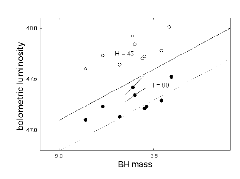
Figure 1: A sample of luminous AI quasars in the $z$ interval $0.6\div 1.5$ in the $\log L_{\mathrm{bol}}$ vs. $\log M_{\mathrm{BH}}$ diagram for two values of $H_{0}$ in the world model $(\Omega_{\mathrm{m}},\Omega_{\Lambda})$ = (0.3,0.7). The upper line indicates the Eddington luminosity, the lower line is $0.5L_{\mathrm{Edd}}$. A change of $H_{0}$ causes a vertical shift. For two quasars we show how $\Delta\Omega_{\Lambda}=\pm 0.15$ in the flat model influences their positions. If these quasars are radiating at $L_{Edd}$ or less, then for the numerical factors used for calculating $L_{bol}$ and $M_{BH}$, 45 kms^-1/Mpc is a strict lower limit for the Hubble constant.

If we change $\Omega_{\Lambda}$ by $\pm 0.15$ (keeping $\Omega_{\mathrm{tot}}=1$), taking the $\sim 2\sigma$ error bars from SNIa’s (Tonry et al. 2003; Knop et al. 2003), one sees just a small dependence of the Eddington ratio on $\Delta\Omega_{\Lambda}$ in Fig.1, where for two quasars are indicated the position shifts for $\Delta\Omega_{\Lambda}=\pm 0.15$. The steeper slope corresponds to $\alpha=0.5$, the shallower one to $\alpha=0.7$.

6 Concluding remarks

Though presently this approach does not add much independent information about the distance scale, it is noteworthy that the natural assumption that $L\leq L_{Edd}$ for the considered quasars leads to a lower limit $h>0.5$ when the usual values of the parameters are used in the calculation of the BH mass and bolometric luminosity. Hence at least a consistent picture emerges.

There is still room for high-$z$ methods to study $H_{0}$ bypassing the local distance ladder, complementing those based on the Sunuyaev-Zeldovich effect and the time delay in gravitational lens images. Furthermore, there are still problems with the local Cepheid-based distance scale (Paturel & Teerikorpi 2005). In the present paper we have shown how the study of the Eddington efficiency is also interestingly connected with the problem of the global distance scale, when in the range $0.5\la z\la 2$ “the Eddington luminosity is still a relevant physical limit to the accretion rate of luminous quasars” (McLure & Dunlop 2004).

References

- (1) Elvis M., Wilkes B.J., McDowell J.C. et al., 1994, ApJSS 95, 1
- (2) Ferrarese L., Merritt D., 2000, ApJ 539, L9
- (3) Gebhardt K., Bender R., Bower G. et al., 2000, ApJ 539, L13
- (4) Kaspi S., Smith P.S., Netzer H., Maoz D., Jannuzi B.T., Giveon U., 2000, ApJ 533, 631
- (5) Knop, R.A., Adering G., Amanullah R., et al., 2003, ApJ 598, 102
- (6) Krolik J.H., 2001, ApJ 551, 72
- (7) McLure R.J., Dunlop J.S., 2001, MNRAS 327, 199
- (8) McLure R.J., Dunlop J.S., 2002, MNRAS 331, 795
- (9) McLure R.J., Dunlop J.S., 2004, MNRAS 352, 1390
- (10) Netzer, H., 1990, in Active Galactic Nuclei, ed. T.J.-L. Courvoisier & M. Mayor (Berlin: Springer), 137
- (11) Netzer H., 2003, ApJ 583, L5
- (12) Paturel G., Teerikorpi P., 2005, A&A (in press)
- (13) Shields G.A., Gebhardt K., Salviander S. et al., 2003, ApJ 583, 124
- (14) Teerikorpi P., 1984, A&A 141, 407
- (15) Teerikorpi P., 1997, ARA&A 35, 101
- (16) Teerikorpi P., 2000, A&A 353, 77
- (17) Tonry J.L., Schmidt B.P., Barris B. et al., 2003, ApJ 594,1
- (18) Vestergaard M., 2002, ApJ 571, 733
- (19) Vestergaard M., 2004, ApJ 601, 676
- (20) Warner C., Hamann F., Dietrich M., 2004, ApJ 608, 136
- (21) Woo J.-H., Urry C.M., 2002, ApJ 579, 530