EFI-0518
Cosmological Structure Evolution and CMB Anisotropies in DGP Braneworlds

Abstract

The braneworld model of Dvali, Gabadadze and Porrati (DGP) provides an intriguing modification of gravity at large distances and late times. By embedding a three-brane in an uncompactified extra dimension with separate Einstein-Hilbert terms for both brane and bulk, the DGP model allows for an accelerating universe at late times even in the absence of an explicit vacuum energy. We examine the evolution of cosmological perturbations on large scales in this theory. At late times, perturbations enter a DGP regime in which the effective value of Newton’s constant increases as the background density diminishes. This leads to a suppression of the integrated Sachs-Wolfe effect, bringing DGP gravity into slightly better agreement with WMAP data than conventional $\Uplambda$CDM. However, we find that this is not enough to compensate for the significantly worse fit to supernova data and the distance to the last-scattering surface in the pure DGP model. $\Uplambda$CDM is, therefore, a better fit.

1 Introduction

It appears that the acceleration of the expansion of the Universe is now indubitable: it has been independently corroborated by measurements of type Ia supernovae [1, 2, 3] and cosmic microwave background radiation observations by the WMAP satellite [4].

The simplest explanation for such an effect is the existence of a positive cosmological constant. Unfortunately, the estimates for its natural value are at least 55 orders of magnitude too large (see [5, 6, 7] for a review). Another possibility is that the vacuum energy is zero, and the dark energy comes from the potential of a slowly-rolling scalar field [8, 9, 10, 11, 12, 13, 14, 15, 16, 17, 18]. Yet another alternative is to modify general relativity so that the effective Friedmann equation predicts cosmic acceleration even in the absence of dark energy. [19, 20]. A simple approach along these lines is to add an $R^{n}$ term to the Einstein–Hilbert action, with $n<0$, which will affect the cosmological dynamics in the infrared.[21]

The case we will discuss in this work is that proposed by Dvali, Gabadadze and Porrati (“DGP”) [22, 23, 24] who suggest that the observed universe might be a brane embedded in a higher-dimensional space-time, with Standard-Model fields propagating strictly on the brane. Gravity propagates in the bulk, but on-brane radiative corrections to the graviton propagator result in there being induced an additional, four-dimensional Ricci scalar in the action. The cosmological solution to this theory with a five-dimensional bulk has been demonstrated to possess a “self-accelerated” branch, as the universe approaches a de Sitter phase even when the vacuum energy vanishes in both the bulk and on the brane. [25].

By finding the equation governing the growth of radially symmetric perturbations on a cosmological background with zero cosmological constants (bulk and brane), Lue et al. [26] conclude that the growth of structure is suppressed in a manner inconsistent with observations and, in the linear regime, the DGP theory is a theory with a varying gravitational constant.

On the other hand, Ishak et al. [27] have simulated data sets for CMB and weak lensing, assuming that the cosmology is pure DGP, and they have found that, if such data are analysed assuming that the cosmological acceleration is driven by a form of dark energy, rather than a modification of gravity, the forms of best-fit $w$ obtained from the two data sets are inconsistent.

Attacking the problem with more generality and a using a different methodology, we show that the quantity which is measured as Newton’s constant for a small perturbation in the Robertson–Walker background is dependent on the energy-density content of the universe and is, in general, not equal to the (truly constant) gravitational constant driving the Friedmann expansion. This effect results in a change in the evolution of gravitational potentials in cosmological models using linear perturbation theory: the matter power spectrum is somewhat altered and the integrated Sachs-Wolfe (ISW) effect is much weakened.

It is well-known that the observed CMB anisotropies have less power on the largest scales than is predicted by the conventional $\Uplambda$CDM model [4, 28, 29]. As a consequence of the suppressed ISW effect, we find that DGP gravity provides a better fit to the temperature anisotropies observed by WMAP than does $\Uplambda$CDM. However, DGP also predicts a somewhat more gradual onset of acceleration than that expected in $\Uplambda$CDM, which is not as good at matching the observed Hubble diagram of Type Ia supernovae if we require that the distance to the last-scattering be fixed. Taken together, we find that although the low-multipole CMB data is significantly better fit by DGP, GR is preferred when both CMB and supernova data are considered for a flat universe.

2 On-Brane Field Equations

We start with a single 3-brane embedded in a five-dimensional bulk $\mathcal{M}$. We will assume that all the standard-model fields are confined to the brane. Gravity propagates in the bulk and is a fully five-dimensional interaction, but, as first proposed in the model of Dvali, Gabadadze and Porrati [22], there is an on-brane radiative correction to the graviton propagator resulting in the induction of an on-brane, four-dimensional Ricci scalar in the effective action. Generalizing the DGP model slightly, we will allow for both a nonzero brane tension, $\lambda$ and bulk cosmological constant, $\Lambda$. No fields propagate in the bulk other than gravity. We thus write down the action:

$$S=\int_{\mathcal{M}}\!\mathrm{d}^{5}x\sqrt{-g}\left[\,\frac{{}^{(5)}R}{2\kappa^{2}}-\Lambda-\frac{K^{+}}{\kappa^{2}}-\frac{K^{-}}{\kappa^{2}}+\delta(\chi)\left(\frac{{}^{(4)}R}{2\mu^{2}}-\lambda+\mathcal{L}_{\text{SM}}\right)\right]\,,$$ (1)

where $g^{\mathchoice{\makebox[4.21783pt][c]{$\displaystyle$}}{\makebox[4.21783pt][c]{$\textstyle$}}{\makebox[2.95248pt][c]{$\scriptstyle$}}{\makebox[2.10892pt][c]{$\scriptscriptstyle$}}\mathchoice{\makebox[3.45787pt][c]{$\displaystyle$}}{\makebox[3.45787pt][c]{$\textstyle$}}{\makebox[2.42052pt][c]{$\scriptstyle$}}{\makebox[1.72893pt][c]{$\scriptscriptstyle$}}}_{\leavevmode{\mu}\leavevmode{\nu}}$ is the metric in the bulk, ${}^{(5)}R$ is the 5D Ricci scalar, ${}^{(4)}R$ is the induced 4D Ricci scalar, $\chi$ parameterizes a vector field such that $\chi=0$ coincides with the position of the brane everywhere (we assume that such a vector field exists); a particular choice for this vector field is $n^{\mu}$, defined in (4). $K^{\pm}$ is the trace of the extrinsic curvature of either side of the brane; this term is the Hawking–Gibbons term necessary to reproduce the appropriate field equations in a space-time with a boundary. The appropriate energy scales are represented by $\kappa^{2}=8\uppi M^{-3}_{5}$ for the true 5D quantum gravity scale and $\mu^{2}=8\uppi M^{-2}_{4}$ for the induced-gravity energy scale on the brane. Finally, $\mathcal{L}_{\text{SM}}$ is the standard-model lagrangian, with fields restricted to the brane.

The ratio of the two gravitational scales, the cross-over scale,

$$r_{\mathrm{c}}:=\frac{\kappa^{2}}{2\mu^{2}}\,,$$ (2)

was shown by Dvali et al. [22] to appear in the propagator of the graviton in the 5D-bulk DGP theory. It is at this distance scale that the potential owing to one-graviton exchange undergoes a transition from 4D to 5D behavior. Also, Deffayet [25] has shown that an FRW cosmology enters a self-accelerated phase when $H\sim r_{\mathrm{c}}^{-1}$. If we wish to explain the cosmological acceleration using this phase, then we need to set $r_{\mathrm{c}}\sim 1$ Gpc, i.e. approximately the current Hubble radius. Dvali et al. [22] show that, at distances much smaller than the critical radius, when expanded around the Minkowski background, $\mu^{2}$ enters the gravitational potential as the constant of proportionality, i.e. $\mu^{2}=8\uppi G$. This forces us to set $M_{4}\equiv M_{\text{Pl}}=10^{28}$ eV and, therefore, $M_{5}=100$ MeV.

Varying the action leads to the following equation of motion:

$${}^{(5)}G^{\leavevmode{\mu}\mathchoice{\makebox[3.45787pt][c]{$\displaystyle$}}{\makebox[3.45787pt][c]{$\textstyle$}}{\makebox[2.42052pt][c]{$\scriptstyle$}}{\makebox[1.72893pt][c]{$\scriptscriptstyle$}}}_{\mathchoice{\makebox[4.21783pt][c]{$\displaystyle$}}{\makebox[4.21783pt][c]{$\textstyle$}}{\makebox[2.95248pt][c]{$\scriptstyle$}}{\makebox[2.10892pt][c]{$\scriptscriptstyle$}}\leavevmode{\nu}}=\kappa^{2}T^{\leavevmode{\mu}\mathchoice{\makebox[3.45787pt][c]{$\displaystyle$}}{\makebox[3.45787pt][c]{$\textstyle$}}{\makebox[2.42052pt][c]{$\scriptstyle$}}{\makebox[1.72893pt][c]{$\scriptscriptstyle$}}}_{\mathchoice{\makebox[4.21783pt][c]{$\displaystyle$}}{\makebox[4.21783pt][c]{$\textstyle$}}{\makebox[2.95248pt][c]{$\scriptstyle$}}{\makebox[2.10892pt][c]{$\scriptscriptstyle$}}\leavevmode{\nu}}\,,$$ (3)

where the indices run over all the five dimensions, from 0 to 4. We write down the induced metric on the brane as

$$q_{\mu\nu}=g_{\mu\nu}-n_{\mu}n_{\nu}\,,$$ (4)

with $n_{\mu}$ a spacelike vector field with unit norm, normal to the brane at $\chi=0$. We can then write down the energy-momentum tensor as

$$T_{\mu\nu}=-\Lambda g_{\mu\nu}+S_{\mu\nu}\delta(\chi)\,,$$ (5)

with the on-brane contribution described by

$$S_{\mu\nu}=\tau_{\mu\nu}-\lambda q_{\mu\nu}-\frac{1}{\mu^{2}}\,^{(4)}G_{\mu\nu}\,.$$ (6)

Here, ${}^{(4)}G_{\mu\nu}$ is the Einstein tensor obtained by varying the usual $\int\!\mathrm{d}^{4}x\,^{(4)}R$, restricted to exist on the brane, while $\tau_{\mu\nu}$ is the energy-momentum tensor resulting from varying $\mathcal{L}_{\text{SM}}$ with respect to $q_{\mu\nu}$. As already mentioned, the bulk is empty, save for a cosmological constant $\Lambda$.

We then proceed by following the methodology first proposed by Shiromizu, Maeda and Sasaki [30]: we carry out a $4+1$ decomposition of the theory (3) and calculate the effective on-brane field equations. This result was first obtained by Maeda et al. in [31]. The detailed derivation is presented in Appendix A.

We use the Gauss equation to calculate the Riemann tensor on the brane:

$${}^{(4)}R^{\leavevmode{\alpha}\mathchoice{\makebox[10.6946pt][c]{$\displaystyle$}}{\makebox[10.6946pt][c]{$\textstyle$}}{\makebox[7.48619pt][c]{$\scriptstyle$}}{\makebox[5.34729pt][c]{$\scriptscriptstyle$}}}_{\mathchoice{\makebox[4.4779pt][c]{$\displaystyle$}}{\makebox[4.4779pt][c]{$\textstyle$}}{\makebox[3.13454pt][c]{$\scriptstyle$}}{\makebox[2.23895pt][c]{$\scriptscriptstyle$}}\leavevmode{\beta\gamma\delta}}=\ ^{(5)}R^{\leavevmode{\mu}\mathchoice{\makebox[11.07686pt][c]{$\displaystyle$}}{\makebox[11.07686pt][c]{$\textstyle$}}{\makebox[7.75381pt][c]{$\scriptstyle$}}{\makebox[5.5384pt][c]{$\scriptscriptstyle$}}}_{\mathchoice{\makebox[4.21783pt][c]{$\displaystyle$}}{\makebox[4.21783pt][c]{$\textstyle$}}{\makebox[2.95248pt][c]{$\scriptstyle$}}{\makebox[2.10892pt][c]{$\scriptscriptstyle$}}\leavevmode{\nu\rho\sigma}}q^{\alpha}_{\phantom{\alpha}\mu}q^{\nu}_{\phantom{\nu}\beta}q^{\rho}_{\phantom{\rho}\gamma}q^{\sigma}_{\phantom{\sigma}\delta}+K^{\alpha}_{\phantom{\alpha}\gamma}K_{\beta\delta}-K^{\alpha}_{\phantom{\alpha}\delta}K_{\beta\gamma}\,,$$ (7)

where $K_{\mu\nu}:=q^{\alpha}_{\phantom{\alpha}\mu}q^{\beta}_{\phantom{\beta}\nu}\nabla_{\alpha}n_{\beta}$ is the extrinsic curvature of the brane. We can compute this curvature by assuming a $Z_{2}$ symmetry of the codimension; using the Israel junction conditions for the jumps in the induced metric and the extrinsic curvature across the brane [32], we obtain

$$2q_{\mu\nu}^{+} =q_{\mu\nu}^{+}-q_{\mu\nu}^{-}=:[q_{\mu\nu}]=0$$ (8)

$$2K_{\mu\nu}^{+} =[K_{\mu\nu}]=-\kappa^{2}\left(S_{\mu\nu}-\frac{1}{3}q_{\mu\nu}S\right)\,.$$ (9)

We now contract (7) appropriately and, after some manipulation, we obtain the equation for the 4D Einstein tensor:

$$\left(1+\frac{\lambda\kappa^{4}}{6\mu^{2}}\right)\ ^{(4)}G_{\mu\nu} =-\left(\frac{\kappa^{2}}{2}\Lambda+\frac{\kappa^{4}\lambda^{2}}{12}\right)q_{\mu\nu}+\frac{\lambda\kappa^{4}}{6}\tau_{\mu\nu}+\frac{\kappa^{4}}{\mu^{4}}f_{\mu\nu}-E_{\mu\nu}\,,$$ (10)

where the tensors $f_{\mu\nu}$ and $E_{\mu\nu}$ are defined as

$$f_{\mu\nu} :=\frac{1}{12}AA_{\mu\nu}-\frac{1}{4}A^{\mathchoice{\makebox[4.21783pt][c]{$\displaystyle$}}{\makebox[4.21783pt][c]{$\textstyle$}}{\makebox[2.95248pt][c]{$\scriptstyle$}}{\makebox[2.10892pt][c]{$\scriptscriptstyle$}}\leavevmode{\alpha}}_{\leavevmode{\mu}\mathchoice{\makebox[4.4779pt][c]{$\displaystyle$}}{\makebox[4.4779pt][c]{$\textstyle$}}{\makebox[3.13454pt][c]{$\scriptstyle$}}{\makebox[2.23895pt][c]{$\scriptscriptstyle$}}}A_{\nu\alpha}+\frac{1}{8}q_{\mu\nu}\left(A_{\alpha\beta}A^{\alpha\beta}-\frac{1}{3}A^{2}\right)$$ (11)

$$E_{\mu\nu} =\ ^{(5)}C^{\leavevmode{\perp}\mathchoice{\makebox[4.4779pt][c]{$\displaystyle$}}{\makebox[4.4779pt][c]{$\textstyle$}}{\makebox[3.13454pt][c]{$\scriptstyle$}}{\makebox[2.23895pt][c]{$\scriptscriptstyle$}}\mathchoice{\makebox[5.25pt][c]{$\displaystyle$}}{\makebox[5.25pt][c]{$\textstyle$}}{\makebox[3.67499pt][c]{$\scriptstyle$}}{\makebox[2.625pt][c]{$\scriptscriptstyle$}}\mathchoice{\makebox[3.95938pt][c]{$\displaystyle$}}{\makebox[3.95938pt][c]{$\textstyle$}}{\makebox[2.77156pt][c]{$\scriptstyle$}}{\makebox[1.97969pt][c]{$\scriptscriptstyle$}}}_{\mathchoice{\makebox[5.25pt][c]{$\displaystyle$}}{\makebox[5.25pt][c]{$\textstyle$}}{\makebox[3.67499pt][c]{$\scriptstyle$}}{\makebox[2.625pt][c]{$\scriptscriptstyle$}}\leavevmode{\alpha}\leavevmode{\perp}\leavevmode{\beta}}q^{\leavevmode{\alpha}\mathchoice{\makebox[4.21783pt][c]{$\displaystyle$}}{\makebox[4.21783pt][c]{$\textstyle$}}{\makebox[2.95248pt][c]{$\scriptstyle$}}{\makebox[2.10892pt][c]{$\scriptscriptstyle$}}}_{\mathchoice{\makebox[4.4779pt][c]{$\displaystyle$}}{\makebox[4.4779pt][c]{$\textstyle$}}{\makebox[3.13454pt][c]{$\scriptstyle$}}{\makebox[2.23895pt][c]{$\scriptscriptstyle$}}\leavevmode{\mu}}q^{\leavevmode{\beta}\mathchoice{\makebox[3.45787pt][c]{$\displaystyle$}}{\makebox[3.45787pt][c]{$\textstyle$}}{\makebox[2.42052pt][c]{$\scriptstyle$}}{\makebox[1.72893pt][c]{$\scriptscriptstyle$}}}_{\mathchoice{\makebox[3.95938pt][c]{$\displaystyle$}}{\makebox[3.95938pt][c]{$\textstyle$}}{\makebox[2.77156pt][c]{$\scriptstyle$}}{\makebox[1.97969pt][c]{$\scriptscriptstyle$}}\leavevmode{\nu}}\,,$$ (12)

with

$$A_{\mu\nu}:=\ ^{(4)}G_{\mu\nu}-\mu^{2}\tau_{\mu\nu}\,.$$ (13)

$E_{\mu\nu}$ is the projection onto the brane of the bulk Weyl tensor ${}^{(5)}C^{\leavevmode{\alpha}\mathchoice{\makebox[10.6946pt][c]{$\displaystyle$}}{\makebox[10.6946pt][c]{$\textstyle$}}{\makebox[7.48619pt][c]{$\scriptstyle$}}{\makebox[5.34729pt][c]{$\scriptscriptstyle$}}}_{\mathchoice{\makebox[4.4779pt][c]{$\displaystyle$}}{\makebox[4.4779pt][c]{$\textstyle$}}{\makebox[3.13454pt][c]{$\scriptstyle$}}{\makebox[2.23895pt][c]{$\scriptscriptstyle$}}\leavevmode{\beta\gamma\delta}}$ ($\perp$ signifies an index contracted with $n_{\mu}$). $f_{\mu\nu}$ describes brane terms that are quadratic in $\tau_{\mu\nu}$ and $G_{\mu\nu}$; henceforth we will drop the superscript ⁽⁴⁾ and assume all quantities are four-dimensional unless otherwise specified. In Appendix A we explicitly define the cross terms appearing in $f_{\mu\nu}$ as $\pi_{\mu\nu}$, $\gamma_{\mu\nu}$ and $\xi_{\mu\nu}$; see equations (64)—(66) for precise definitions.

We can recover the standard Einstein equations from (10) by sending the brane tension $\lambda$ to infinity, i.e. in the limit when the brane is ‘stiff’.

The difference between DGP gravity and the standard Randall–Sundrum result of [30] is the presence of the 4D Einstein tensor in $S_{\mu\nu}$, resulting in additional terms containing ${}^{(4)}G_{\mu\nu}$ explicitly: we now have an equation which is quadratic in the Einstein tensor, i.e. curvature can act as a source of curvature, leading to a potentially non-zero Ricci in the vacuum (as obtained, for example, by Gabadadze and Iglesias in [33, 34] for their Schwarzschild-like solution in DGP).

3 Cosmological Solution

The quadratic nature of (10) makes this formulation computationally imposing. In addition, it was already noted by Shiromizu et al. in [30] that the transverse-traceless component of $E_{\mu\nu}$ contains the information about gravitational radiation coming off and onto the brane as well as the transition from 4D to 5D gravity, and its evolution is necessarily dependent on the state of the bulk: the equation of motion for $E_{\mu\nu}$ does not close on the brane.

Nevertheless, the large symmetry of a Robertson-Walker universe allows us to make progress. Choosing Gaussian normal co-ordinates, with the brane positioned at $y=0$ and a Robertson–Walker metric on the brane, our bulk metric becomes:

$$ds^{2}=-N^{2}(y)dt^{2}+A^{2}(t,y)\gamma_{ij}dx^{i}dx^{j}+dy^{2}\,,$$ (14)

and we are allowed to pick the normalization such that $N(0)=1$ by rescaling the time variable; $\gamma_{ij}$ is a 3D maximally-symmetric spatial metric. We also define the value of $A$ on the brane: $a(t):=A(t,0)$. In these coordinates, the 4D tensors are significantly simplified, with only zero entries in the columns and rows corresponding to the dimension perpendicular to the brane. We thus obtain for $G^{\leavevmode{\mu}\mathchoice{\makebox[3.45787pt][c]{$\displaystyle$}}{\makebox[3.45787pt][c]{$\textstyle$}}{\makebox[2.42052pt][c]{$\scriptstyle$}}{\makebox[1.72893pt][c]{$\scriptscriptstyle$}}}_{\mathchoice{\makebox[4.21783pt][c]{$\displaystyle$}}{\makebox[4.21783pt][c]{$\textstyle$}}{\makebox[2.95248pt][c]{$\scriptstyle$}}{\makebox[2.10892pt][c]{$\scriptscriptstyle$}}\leavevmode{\nu}}$:

$$G^{\leavevmode{0}\mathchoice{\makebox[3.5pt][c]{$\displaystyle$}}{\makebox[3.5pt][c]{$\textstyle$}}{\makebox[2.45pt][c]{$\scriptstyle$}}{\makebox[1.75pt][c]{$\scriptscriptstyle$}}}_{\mathchoice{\makebox[3.5pt][c]{$\displaystyle$}}{\makebox[3.5pt][c]{$\textstyle$}}{\makebox[2.45pt][c]{$\scriptstyle$}}{\makebox[1.75pt][c]{$\scriptscriptstyle$}}\leavevmode{0}} =-3\left(\frac{\dot{a}^{2}}{a^{2}}+\frac{k}{a^{2}}\right)$$ (15)

$$G^{\leavevmode{i}\mathchoice{\makebox[3.28334pt][c]{$\displaystyle$}}{\makebox[3.28334pt][c]{$\textstyle$}}{\makebox[2.29834pt][c]{$\scriptstyle$}}{\makebox[1.64166pt][c]{$\scriptscriptstyle$}}}_{\mathchoice{\makebox[2.41159pt][c]{$\displaystyle$}}{\makebox[2.41159pt][c]{$\textstyle$}}{\makebox[1.68811pt][c]{$\scriptstyle$}}{\makebox[1.2058pt][c]{$\scriptscriptstyle$}}\leavevmode{j}} =-\left(2\frac{\ddot{a}}{a}+\frac{\dot{a}^{2}}{a^{2}}+\frac{k}{a^{2}}\right)\delta^{\leavevmode{i}\mathchoice{\makebox[3.28334pt][c]{$\displaystyle$}}{\makebox[3.28334pt][c]{$\textstyle$}}{\makebox[2.29834pt][c]{$\scriptstyle$}}{\makebox[1.64166pt][c]{$\scriptscriptstyle$}}}_{\mathchoice{\makebox[2.41159pt][c]{$\displaystyle$}}{\makebox[2.41159pt][c]{$\textstyle$}}{\makebox[1.68811pt][c]{$\scriptstyle$}}{\makebox[1.2058pt][c]{$\scriptscriptstyle$}}\leavevmode{j}}$$ (16)

$$G^{\leavevmode{\mu}\mathchoice{\makebox[4.21783pt][c]{$\displaystyle$}}{\makebox[4.21783pt][c]{$\textstyle$}}{\makebox[2.95248pt][c]{$\scriptstyle$}}{\makebox[2.10892pt][c]{$\scriptscriptstyle$}}}_{\mathchoice{\makebox[4.21783pt][c]{$\displaystyle$}}{\makebox[4.21783pt][c]{$\textstyle$}}{\makebox[2.95248pt][c]{$\scriptstyle$}}{\makebox[2.10892pt][c]{$\scriptscriptstyle$}}\leavevmode{\mu}} =-6\left(\frac{\ddot{a}}{a}+\frac{\dot{a}^{2}}{a^{2}}+\frac{k}{a^{2}}\right)\,,$$ (17)

with the dot representing differentiation with respect to the $t$ coordinate. In addition, we assume that the brane is filled with a homogeneous distribution of a perfect fluid, such that

$$\tau^{\leavevmode{\mu}\mathchoice{\makebox[3.45787pt][c]{$\displaystyle$}}{\makebox[3.45787pt][c]{$\textstyle$}}{\makebox[2.42052pt][c]{$\scriptstyle$}}{\makebox[1.72893pt][c]{$\scriptscriptstyle$}}}_{\mathchoice{\makebox[4.21783pt][c]{$\displaystyle$}}{\makebox[4.21783pt][c]{$\textstyle$}}{\makebox[2.95248pt][c]{$\scriptstyle$}}{\makebox[2.10892pt][c]{$\scriptscriptstyle$}}\leavevmode{\nu}} =\text{diag}(-\rho,p,p,p,0)\$$ (18)

$$p =w\rho\,.$$ (19)

This allows us to obtain the 0-0 component of the quadratic tensor $f^{\mu}{}_{\nu}$ of (11):

$$f^{0}{}_{0}=-\frac{1}{12}\left[\mu^{2}\rho-3\left(\frac{{\dot{a}}^{2}}{a^{2}}+\frac{k}{a^{2}}\right)\right]^{2}\,.$$ (20)

The remaining issue is the tensor $E_{\mu\nu}$. Since we are dealing with an isotropic and homogeneous universe, we must set it to be just a function of the time on the brane. Since it is traceless, it behaves just like radiation and decays as $a^{-4}$; because of this property, this term is usually referred to as dark radiation (see, for example, the review of Maartens [35]). For the moment we will set:

$$E^{\leavevmode{0}\mathchoice{\makebox[3.5pt][c]{$\displaystyle$}}{\makebox[3.5pt][c]{$\textstyle$}}{\makebox[2.45pt][c]{$\scriptstyle$}}{\makebox[1.75pt][c]{$\scriptscriptstyle$}}}_{\mathchoice{\makebox[3.5pt][c]{$\displaystyle$}}{\makebox[3.5pt][c]{$\textstyle$}}{\makebox[2.45pt][c]{$\scriptstyle$}}{\makebox[1.75pt][c]{$\scriptscriptstyle$}}\leavevmode{0}}=\frac{C}{a^{4}}\,,$$ (21)

although ultimately we will set this term to zero.

Substituting the above into (10) and replacing $\frac{\dot{a}}{a}$ with $H$, we obtain a quadratic equation for the energy density (or, equivalently, for $H^{2}$):

$$\frac{\kappa^{4}}{12}\rho^{2}+\left(\frac{\lambda\kappa^{4}}{6}-\frac{\kappa^{4}}{2\mu^{2}}\left(H^{2}+\frac{k}{a^{2}}\right)\right)\rho+\frac{3}{4}\frac{\kappa^{4}}{\mu^{4}}\left(H^{2}+\frac{k}{a^{2}}\right)^{2}-$$

$$\qquad-3\left(1+\frac{\kappa^{4}\lambda}{6\mu^{2}}\right)\left(H^{2}+\frac{k}{a^{2}}\right)+\frac{\kappa^{2}}{2}\left(\Lambda+\frac{\kappa^{2}\lambda^{2}}{6}\right)+\frac{C}{a^{4}}=0\,,$$ (22)

where $k=-1,1,0$ depending on whether the spatial hypersurface on the brane has negative, positive or no curvature. We can write this relation as a version of the Friedmann equation with modified dependence on the Hubble parameter,

$$H^{2}\pm\frac{2\mu^{2}}{\kappa^{2}}\sqrt{\left(H^{2}+\frac{k}{a^{2}}\right)-\frac{\kappa^{2}}{6}\Lambda-\frac{C}{3a^{4}}}=\frac{\mu^{2}}{3}(\rho+\lambda)-\frac{k}{a^{2}}\,.$$ (23)

So, provided that the $\Lambda$ and $C$ terms remain negligible, and $H^{2}+\frac{k}{a^{2}}\gg 2\frac{\mu^{2}}{\kappa^{2}}$, the evolution of the scale factor in the early universe does not differ from that in standard FRW cosmology. As $H$ decreases the evolution becomes non-standard; this can be demonstrated more clearly by solving (22) for $H^{2}$:

$$H^{2}=2\frac{\mu^{4}}{\kappa^{4}}+\frac{\mu^{2}}{3}(\rho+\lambda)-\frac{k}{a^{2}}+2\epsilon\frac{\mu^{2}}{\kappa^{2}}\sqrt{\frac{\mu^{4}}{\kappa^{4}}+\frac{\mu^{2}}{3}(\rho+\lambda)-\frac{\kappa^{2}}{6}\Lambda-\frac{C}{3a^{4}}}\,,$$ (24)

with $\epsilon=\pm 1$ representing the two possible embeddings of the brane in the bulk (see [25]). The above result has been obtained previously obtained by Collins and Holdom [36] and Shtanov [37].

We are going to follow Deffayet [25] by naming the $\epsilon=+1$ branch as ‘self-accelerated’ and $\epsilon=-1$ branch as ‘non-accelerated’. The reason for this nomenclature becomes obvious in the case of flat bulk and a zero brane tension and no dark radiation, i.e. $k,\lambda,\Lambda,C=0$. Equation (24) then reduces to that originally obtained by Deffayet (ibid):

$$H^{2}=2\frac{\mu^{4}}{\kappa^{4}}+\frac{\mu^{2}}{3}\rho+2\epsilon\frac{\mu^{2}}{\kappa^{2}}\sqrt{\frac{\mu^{4}}{\kappa^{4}}+\frac{\mu^{2}}{3}\rho}\,.$$ (25)

As mentioned previously, this solution contains a cross-over scale above which the self-acceleration term dominates:

$$r_{\mathrm{c}}:=\frac{\kappa^{2}}{2\mu^{2}}\,.$$ (26)

For $\epsilon=+1$, once $\mu^{2}\rho/3\ll r_{\mathrm{c}}^{-2}/2$, $H$ approaches the nonzero constant $r_{\mathrm{c}}^{-1}=2\mu^{2}/\kappa^{2}$, and the universe enters an accelerated de Sitter phase. If we wish to use this model to replace the effects of the cosmological constant, we should set $r_{\mathrm{c}}$ to be approximately the current Hubble radius. The non-accelerated branch with $\epsilon=-1$ behaves like the usual Friedman universe, with $H^{2}$ tending to zero in the flat-universe case.

Note that there are two distinct limits in which we can recover the ordinary Friedmann equation in the presence of a cosmological constant,

$$H^{2}=\frac{\mu^{2}}{3}(\rho+\rho_{\text{vac}})-\frac{k}{a^{2}}\,,$$ (27)

where $\rho$ is the energy density in everything other than the cosmological constant. One limit is to simply let $\kappa^{2}\rightarrow\infty$, decoupling the extra dimension entirely and leaving us with $\rho_{\text{vac}}=\lambda$. The other is to set the brane tension to zero, $\lambda=0$, and take both $\kappa^{2}$ and $-\Lambda$ to infinity while keeping their ratio constant, yielding

$$\rho_{\text{vac}}=\sqrt{-\frac{6\Lambda}{\kappa^{2}}}\,.$$ (28)

In our investigation of DGP cosmology, we will set the brane tension to zero while leaving the bulk cosmological constant $\Lambda$ as a free parameter and calculating its likelihood as determined by the data. Then $\Lambda=0$ corresponds to “pure DGP,” while $\Lambda\rightarrow-\infty$ corresponds to ordinary $\Uplambda$CDM.

4 Linearized Equations and the Potential

In this section, we will derive the Poisson equation for a perturbation of the Robertson–Walker background and demonstrate that it deviates from the usual version: in its linear regime, the DGP theory on the brane is a varying-$G$ theory. This derivation will assume that we are able to neglect all terms not linear in the gravitational potential. This range of validity of this assumption is discussed in §5.

We start off by introducing scalar perturbations to the metric. Since we are only going to be dealing with on-brane directions, we can use the 4D formalism in the conformal Newtonian gauge, parameterizing the perturbed metric by:

$$ds^{2}=-(1+2\Psi(\boldsymbol{x},t))dt^{2}+a(t)(1+2\Phi(\boldsymbol{x},t))\gamma_{ij}dx^{i}dx^{j}\,.$$ (29)

This allows us to calculate the Einstein tensor up to first order in the perturbations:

$$G^{\leavevmode{0}\mathchoice{\makebox[3.5pt][c]{$\displaystyle$}}{\makebox[3.5pt][c]{$\textstyle$}}{\makebox[2.45pt][c]{$\scriptstyle$}}{\makebox[1.75pt][c]{$\scriptscriptstyle$}}}_{\mathchoice{\makebox[3.5pt][c]{$\displaystyle$}}{\makebox[3.5pt][c]{$\textstyle$}}{\makebox[2.45pt][c]{$\scriptstyle$}}{\makebox[1.75pt][c]{$\scriptscriptstyle$}}\leavevmode{0}}=-3H^{2}+6H^{2}\Psi-6H\dot{\Phi}+\frac{2}{a^{2}}\boldsymbol{\nabla}^{2}\Phi+\mathcal{O}(\Phi^{2},\Psi^{2})\,.$$ (30)

The above approximation is permitted provided $\Phi,\Psi\ll 1$. If we consider distance scales much smaller than Hubble scale, i.e. upon taking the Fourier transform, $(k/a)^{2}\Phi\gg H^{2}\Psi,H\dot{\Phi}$, then from the first-order terms we recover the potential for the flat Minkowski spacetime:

$${}^{(1)}G^{\leavevmode{0}\mathchoice{\makebox[3.5pt][c]{$\displaystyle$}}{\makebox[3.5pt][c]{$\textstyle$}}{\makebox[2.45pt][c]{$\scriptstyle$}}{\makebox[1.75pt][c]{$\scriptscriptstyle$}}}_{\mathchoice{\makebox[3.5pt][c]{$\displaystyle$}}{\makebox[3.5pt][c]{$\textstyle$}}{\makebox[2.45pt][c]{$\scriptstyle$}}{\makebox[1.75pt][c]{$\scriptscriptstyle$}}\leavevmode{0}}=\frac{2}{a^{2}}\boldsymbol{\nabla}^{2}\Phi\,.$$ (31)

Alternatively, by including the Hubble flow, we can obtain the 0-0 component of the cosmological evolution equation for the gravitational potentials in GR:

$$\frac{1}{a^{2}}\boldsymbol{\nabla}^{2}\Phi+3H^{2}\Psi-3H\dot{\Phi}=-\frac{\mu^{2}}{2}\bar{\rho}\delta$$ (32)

where $\bar{\rho}$ is the average matter/radiation energy density of the universe, $\delta\rho$ is the deviation from this mean, and the fractional density excess is defined as $\delta:=\delta\rho/\bar{\rho}$.

In DGP gravity, the 0-0 component of the right-hand side of the modified Einstein equation (10), first-order in $\Phi$ or $\Psi$, is:

$${}^{(1)}[\text{RHS}]^{\leavevmode{0}\mathchoice{\makebox[3.5pt][c]{$\displaystyle$}}{\makebox[3.5pt][c]{$\textstyle$}}{\makebox[2.45pt][c]{$\scriptstyle$}}{\makebox[1.75pt][c]{$\scriptscriptstyle$}}}_{\mathchoice{\makebox[3.5pt][c]{$\displaystyle$}}{\makebox[3.5pt][c]{$\textstyle$}}{\makebox[2.45pt][c]{$\scriptstyle$}}{\makebox[1.75pt][c]{$\scriptscriptstyle$}}\leavevmode{0}} =-\delta\rho\frac{\kappa^{4}}{6}\left(\lambda+\bar{\rho}\right)+\frac{\kappa^{4}}{\mu^{2}}H\dot{\Phi}-\frac{3\kappa^{4}}{\mu^{4}}\left(H^{3}\dot{\Phi}+H^{4}\Psi\right)+\frac{\kappa^{4}}{2\mu^{2}}(\delta\rho-2\bar{\rho}\Psi)H^{2}$$

$$\qquad+\left(\frac{\kappa^{4}}{\mu^{4}}H^{2}-\frac{\kappa^{4}\bar{\rho}}{3\mu^{2}}\right)a^{-2}\boldsymbol{\nabla}^{2}\Phi\,.$$ (33)

In calculating the above, we have assumed that the effect of the perturbations of the Weyl tensor, $E_{\mu\nu}$ in this equation at sub-horizon scales are insignificant. Since we are dealing with a quasi-static situation, gravitational radiation is negligible. In addition, this tensor encodes the transition of gravity from 4D to 5D behavior. However, this effect only occurs at a length scale determined by $r_{\mathrm{c}}$, which, as shown in the data fits of §6.2, is much larger than the horizon scale even today, let alone in the past. As such, it is unlikely to have any significant effect on the quantities under consideration.

Performing some algebraic manipulation and substituting for $H^{2}$ from (24) we obtain the DGP equivalent of (32):

$$\frac{1}{a^{2}}\boldsymbol{\nabla}^{2}\Phi+3H^{2}\Psi-3H\dot{\Phi}=-\frac{\mu^{2}}{2}\bar{\rho}\left(1+\frac{\epsilon}{\sqrt{1+\frac{4}{3}\mu^{2}r_{\mathrm{c}}^{2}\left(\bar{\rho}+\lambda-r_{\mathrm{c}}\Lambda-\frac{\kappa^{4}C}{\mu^{4}a^{4}}\right)}}\right)\delta$$ (34)

If we apply similar approximations to those that led to (31), i.e. assuming that $\Phi,\Psi\ll 1$, drop terms containing $H$ by considering scales over which the Hubble flow is negligible, we obtain:

$$\boldsymbol{\nabla}^{2}\Phi=-\frac{\mu^{2}\bar{\rho}a^{2}}{2}\left(1+\frac{\epsilon}{\sqrt{1+\frac{4}{3}\mu^{2}r_{\mathrm{c}}^{2}\left(\bar{\rho}+\lambda-r_{\mathrm{c}}\Lambda-\frac{\kappa^{4}C}{\mu^{4}a^{4}}\right)}}\right)\delta\,.$$ (35)

This form of (35) signifies that the weak-field approximation in a Robertson–Walker background is a varying-$G$ theory, with the effective Newton’s constant dependent on the average energy density of the Universe:

$$G_{\text{eff}}=\frac{\mu^{2}}{8\uppi}\left(1+\frac{\epsilon}{\sqrt{1+\frac{4}{3}\mu^{2}r_{\mathrm{c}}^{2}\left(\bar{\rho}+\lambda-r_{\mathrm{c}}\Lambda-\frac{3C}{a^{4}\mu^{2}}\right)}}\right)\,.$$ (36)

Note that, in the numerical solutions described below, we do not neglect terms containing $H$; we are taking that limit here purely for expository purposes.

The large-scale evolution of the universe is always driven by (24), i.e. the energy scale encoded in $\mu^{2}$. This is the parameter which drives the conditions during, for example, nucleosynthesis. However, at least in part, the evolution of structure is driven by the effective Newton’s constant, i.e. equation (36): this is generally true at late times for diffuse clouds of gas. This insight will provide a constraint for some of the parameters of the theory.

As we can observe from equation (36) and assuming that we are in the self-accelerated branch of the solution ($\epsilon=+1$), the value of the effective $G_{\text{eff}}$ varies from one to, at most, two times the underlying Newton’s constant, with the increase occurring in the late universe as $\bar{\rho}\rightarrow 0$. (A related effect has been observed in the presence of Lorentz-violating vector fields [38], which result in a cosmology where Newton’s constant differs from the constant relating energy density to the Hubble parameter in the Friedmann equation.) In the limit described at the end of section 3, in which we take $\Lambda\rightarrow-\infty$, the time-dependent piece of $G_{\text{eff}}$ goes away, and we obtain $G_{\text{eff}}=\mu^{2}/8\uppi=$ constant, so that ordinary $\Uplambda$CDM is indeed recovered.

By considering the $i$–$j$ equations of motion in GR, we can get the an equation relating the two potentials $\Phi$ and $\Psi$ to the anisotropic stress of the cosmological fluid, $\pi$:

$$\frac{k^{2}}{a^{2}}(\Phi+\Psi)=\mu^{2}\pi$$ (37)

Since the anisotropic stress is negligible in models with no neutrinos, we can set $\Phi=-\Psi$. The analogous calculation in DGP is a little more complex; however, it yields similar results: without a source of significant anisotropic stress in the cosmological fluid, we can set $\Phi=-\Psi$.

$$\left(1+\frac{\kappa^{2}}{6\mu^{2}}\left(\lambda+\frac{1}{2}\bar{\rho}(1-3w)-\frac{3\ddot{a}}{\mu^{2}a}\right)\right)\frac{k^{2}}{a^{2}}(\Phi+\Psi)=$$ (38)

$$=\frac{\kappa^{2}}{6\mu^{2}}\left(\lambda+\frac{1}{2}\bar{\rho}(1-3w)-\frac{3\ddot{a}}{\mu^{2}a}\right)\mu^{2}\pi-\pi_{E}$$

$\pi_{E}$ is a new term and is the anisotropic stress encoded in the the Weyl tensor $E_{\mu\nu}$, i.e. a result of off-brane effects, such as graviton evaporation into the bulk and any gravitational waves going off or coming onto the brane. We will set this to zero in the subsequent analysis.

5 Range of Validity of Linear Regime

In section 4, we assumed that we can use the linear approximation to the modified Einstein’s equation (10). It is important to verify this explicitly, since the large magnitude of the coefficients of the quadratic terms in (10), might lead to their dominating over the linear terms.

After a systematic review of all the quadratic terms in the expansion of (10), we conclude that the quadratic term which is most likely to be large arises from the $(G^{\mathchoice{\makebox[4.21783pt][c]{$\displaystyle$}}{\makebox[4.21783pt][c]{$\textstyle$}}{\makebox[2.95248pt][c]{$\scriptstyle$}}{\makebox[2.10892pt][c]{$\scriptscriptstyle$}}\mathchoice{\makebox[3.45787pt][c]{$\displaystyle$}}{\makebox[3.45787pt][c]{$\textstyle$}}{\makebox[2.42052pt][c]{$\scriptstyle$}}{\makebox[1.72893pt][c]{$\scriptscriptstyle$}}}_{\leavevmode{\mu}\leavevmode{\nu}})^{2}$ term and is of the form

$$\frac{\kappa^{4}}{\mu^{4}}\left(\boldsymbol{\nabla}^{2}\Phi\right)^{2}$$ (39)

Assuming that the Poisson equation is approximately valid, despite the evolving cosmological background, we have $\boldsymbol{\nabla}^{2}\Phi\sim\mu^{2}\bar{\rho}\delta$, and using the definition of $r_{\mathrm{c}}$, (26), leads to the condition that for the linearization of DGP to be valid

$$r^{2}_{\mathrm{c}}\mu^{2}\bar{\rho}\delta\ll 1$$ (40)

If we assume that the density perturbation is in the form of a spherical top hat with a characteristic size $D$, we can write down the mass of this object as $M\sim D^{3}\bar{\rho}\delta$. Finally, the Schwarzschild radius in four dimensions is $r_{\mathrm{S}}\sim\mu^{2}M$, giving us:

$$r^{2}_{\mathrm{c}}r_{\mathrm{S}}\ll D^{3}$$ (41)

We have thus recovered the result first discovered by Dvali et al [39], that there is a new scale in DGP theory,

$$r_{*}=(r_{\mathrm{c}}^{2}r_{\mathrm{S}})^{1/3}\,.$$ (42)

At small distances (between the Schwarzschild radius and $r_{*}$), gravity behaves essentially as in 4D GR, because the quadratic terms dominate the modified Einstein equation (10). If we set $\Lambda=\lambda=0$, in this regime we are looking for the solution to

$$f^{\leavevmode{\mu}\mathchoice{\makebox[3.45787pt][c]{$\displaystyle$}}{\makebox[3.45787pt][c]{$\textstyle$}}{\makebox[2.42052pt][c]{$\scriptstyle$}}{\makebox[1.72893pt][c]{$\scriptscriptstyle$}}}_{\mathchoice{\makebox[4.21783pt][c]{$\displaystyle$}}{\makebox[4.21783pt][c]{$\textstyle$}}{\makebox[2.95248pt][c]{$\scriptstyle$}}{\makebox[2.10892pt][c]{$\scriptscriptstyle$}}\leavevmode{\nu}}\approx 0$$ (43)

with the obvious solution being $G^{\leavevmode{\mu}\mathchoice{\makebox[3.45787pt][c]{$\displaystyle$}}{\makebox[3.45787pt][c]{$\textstyle$}}{\makebox[2.42052pt][c]{$\scriptstyle$}}{\makebox[1.72893pt][c]{$\scriptscriptstyle$}}}_{\mathchoice{\makebox[4.21783pt][c]{$\displaystyle$}}{\makebox[4.21783pt][c]{$\textstyle$}}{\makebox[2.95248pt][c]{$\scriptstyle$}}{\makebox[2.10892pt][c]{$\scriptscriptstyle$}}\leavevmode{\nu}}=\mu^{2}\tau^{\leavevmode{\mu}\mathchoice{\makebox[3.45787pt][c]{$\displaystyle$}}{\makebox[3.45787pt][c]{$\textstyle$}}{\makebox[2.42052pt][c]{$\scriptstyle$}}{\makebox[1.72893pt][c]{$\scriptscriptstyle$}}}_{\mathchoice{\makebox[4.21783pt][c]{$\displaystyle$}}{\makebox[4.21783pt][c]{$\textstyle$}}{\makebox[2.95248pt][c]{$\scriptstyle$}}{\makebox[2.10892pt][c]{$\scriptscriptstyle$}}\leavevmode{\nu}}$, i.e. the usual 4D Einstein equation. On intermediate scales (between $r_{*}$ and $r_{\mathrm{c}}$), gravity is described by a scalar-tensor theory, consistent with our description above in terms of a time-dependent gravitational constant. It is in this regime that the linearized DGP equations are valid.

As we will see below, as a perturbation of fixed comoving size expands along with the universe, it typically goes from being less than $r_{*}$ to being greater than $r_{*}$. Each mode is therefore described by 4D GR at early times, and later on by linearized DGP.

6 Cosmological Simulations

6.1 The Simulation

In order to test the effects on cosmological observations of modifying gravity, we built a simple cosmological simulation containing only dark matter and radiation and modeled their evolution according to linearized equations – linearized DGP or ordinary 4D GR, depending on the regime a given mode is in. The model produces as outputs the matter power spectrum and the contribution of the Sachs–Wolfe effect (both integrated and non-integrated) to the radiation power spectrum. The difference between the matter power spectra is slight; however, the impact on the ISW is significant, resulting in a large reduction of power at low multipoles.

We compare the results of the concordance $\Uplambda$CDM model to that of DGP cosmology. The concordance model is defined by $\Omega_{\mathrm{m}}=0.27$, $\Omega_{\mathrm{m}}/\Omega_{\mathrm{r}}=3234$ and $\Omega_{\lambda}+\Omega_{\mathrm{m}}+\Omega_{\mathrm{r}}=1$. For the DGP cosmologies we use the same matter to radiation energy ratio, and choose the self-accelerated embedding, $\epsilon=+1$. We keep $\Omega_{\mathrm{r}}h^{2}$ constant. As our aim is to explain the acceleration of the expansion of the universe using effects arising from modified gravity, we have set the brane tension $\lambda$ (which is equivalent to the cosmological constant in $\Uplambda$CDM) to zero in all our considerations. For simplicity we have also set $C$ and $k$ to zero, i.e. we are assuming a flat cosmology. We keep the bulk cosmological constant $\Lambda$ as a free parameter.

We parameterize the DGP models by rewriting (24) as:

$$\frac{H^{2}}{H_{0}^{2}}=\frac{1}{2\beta^{2}}+\Omega_{\mathrm{m}}a^{-3}+\Omega_{\mathrm{r}}a^{-4}+\frac{1}{\beta}\sqrt{\frac{1}{4\beta^{2}}+\Omega_{\mathrm{m}}a^{-3}+\Omega_{\mathrm{r}}a^{-4}-\Omega_{\Lambda}}$$ (44)

where $H_{0}$ is the Hubble parameter today,

$$\beta:=r_{\mathrm{c}}H_{0}\qquad$$ cross-over radius in Hubble units

$$\Omega_{\mathrm{m}}+\Omega_{\mathrm{r}}:=\mu^{2}\bar{\rho}_{0}/3H_{0}^{2}=1-\beta^{-1}\sqrt{1-\Omega_{\Lambda}}$$ energy density

$$\Omega_{\Lambda}:=\kappa^{2}\Lambda/6H_{0}^{2}\qquad$$ dimensionless bulk cosmological constant

$$\Omega_{\mathrm{r}}=\Omega_{\mathrm{m}}/3234\qquad$$ fractional radiation density

$\Omega_{\mathrm{m}}$ is the contribution of matter to the total energy density of the universe (the remainder coming from the DGP curvature). Realistic DGP models will have $\Omega_{\mathrm{m}}\sim 0.3$, just as in $\Uplambda$CDM. The energy scale for the bulk cosmological constant is $\Lambda\approx(10^{-8}\leavevmode\nobreak\ \text{eV})^{5}\Omega_{\Lambda}$.

A significant issue in modeling DGP is deciding on where the the transition between the Einstein and the linear DGP regimes occurs and how to implement it. The simulation was built to switch from GR to linearized DGP instantaneously at the point in evolution defined by the scale $r_{*}$. We will apply DGP gravity when the scale of the perturbation is

$$D^{3}\sim r_{*}^{3}=2GMr_{\mathrm{c}}^{2}=\frac{1}{24}\mu^{2}D^{3}r_{\mathrm{c}}^{2}\bar{\rho}\delta$$ (45)

The perturbation size is eliminated from the relationship, yielding for the fractional density perturbation at which GR transitions to linear DGP:

$$\delta\sim\frac{24}{\mu^{2}r_{\mathrm{c}}^{2}\bar{\rho}_{0}}a^{3(1+w(a))}$$ (46)

where $w(a)$ is the effective equation of state parameter for the fluid comprising the universe and $a$ is the scale factor; $\delta$ is dependent on the initial conditions, and thus is a function of the mode under consideration. Thus, for matter and radiation, the transition occurs from GR to DGP and occurs only once in the evolution of the perturbations. This transition has been plotted on Figure 1. We can determine the success of the splicing between GR and the linear DGP regimes by comparing the value of the effective Newton’s constant at the transition point. We found that the transition occurs at around $z=20$ for modes of the size of the horizon today, with $G_{\text{eff}}\approx 1.02G$, with this transition occurring at larger redshifts for higher modes and $G_{\text{eff}}$ even closer to 1.

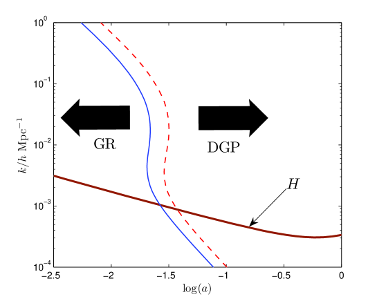
Figure 1: Value of scale factor at which the gravity driving evolution transitions from GR to linear DGP. Solid line is for Minkowski bulk ($\Omega_{\Lambda}=0$), dashed for $\Omega_{\Lambda}=-1$. Shape of transition line is a processed dark-matter power spectrum.

In Figure 2 we plot the evolution of the Newtonian gravitational potential $\Phi$ for different modes in both $\Uplambda$CDM and DGP. Each mode diminishes in amplitude when it first comes into the Hubble radius (more so during radiation domination), before settling to a constant amplitude. In $\Uplambda$CDM, linear modes once again decrease in amplitude when vacuum energy begins to dominate over matter. In DGP, in contrast, the effective gravitational constant increases just when the universe begins to accelerate, leading to an increase in the amplitude of $\Phi$ that can be appreciable for certain wavelengths. This behavior is also reflected in the transfer function for dark matter perturbations, plotted in Figure 3, which shows a slight enhancement in DGP over $\Uplambda$CDM.

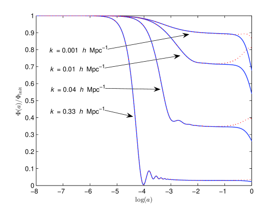
Figure 2: Evolution of Newtonian potential $\Phi$ in GR and DGP (GR— solid lines, DGP—dashed). In DGP, the growth of the effective Newton’s constant leads to a wavelength-dependent growth in the potentials at late times, as opposed to the decay observed in $\Uplambda$CDM. ($\Uplambda$CDM: concordance model; DGP: $\Omega_{\Lambda}=0,\beta=1.38$)

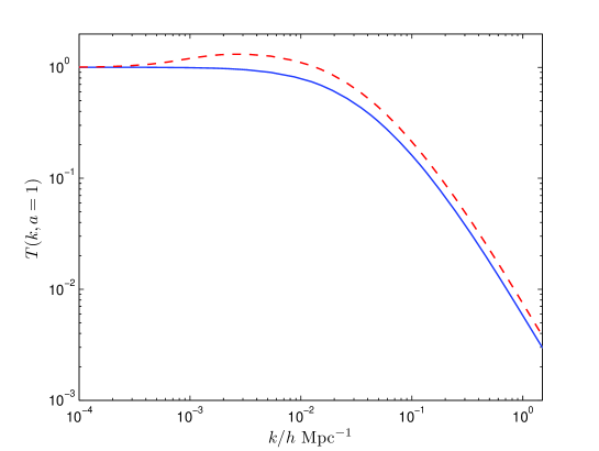
Figure 3: Transfer functions in $\Uplambda$CDM and DGP ($\Omega_{\Lambda}=0$, $\beta=1.38$). The transfer function is defined here as ratio of size of initial perturbation in $\Phi$ to its final value, renormalized to 1 at large scales. In GR, the growth rate for the potential during dark-energy domination is independent of $k$, so the quantity shown here is equivalent to the usual transfer function. For DGP, the growth rate depends on $k$.

6.2 Constraints from Expansion History

Before considering details of CMB anisotropies, we turn to two sources of constraints on the expansion history of the universe: the Hubble diagram of Type Ia supernovae, and the distance to last scattering as measured by WMAP. These imply a tight relationship between the two free parameters in the DGP model: $\beta\equiv r_{c}H_{0}$ and $\Omega_{\Lambda}$. We will then calculate CMB anisotropies in models that obey this relationship.

For the supernova data, we used the Riess et al. Gold SNe Ia data set [40] (156 supernovae) and searched for the parameters minimizing $\chi^{2}$. In the DGP scenario with both $\beta$ and $\Omega_{\Lambda}$ free, the optimization routine chooses very large and negative values for $\Omega_{\Lambda}$, corresponding to the $\Uplambda$CDM limit as discussed at the end of Section 3. The supernova data, in other words, prefer a very large and negative bulk cosmological constant, reducing the observable physics to GR. This is the result of the fact that $\Uplambda$CDM fits the supernova data slightly better (see Table 1). In terms of the effective equation-of-state parameter $w$, the supernova data prefer $w\approx-1$ or even a little less, while pure DGP corresponds to $w_{\text{eff}}\approx-0.7$ today.

If we fix $\Omega_{\Lambda}=0$, supernova data fit best when $\beta=1.20$, implying $\Omega_{\mathrm{m}}=0.20$. The details of the fit are presented in Table 1.

The WMAP experiment has determined, to a high level of precision, the distance to the last-scattering surface as $d_{\text{ls}}=14.0^{+0.2}_{-0.3}$ Gpc $\equiv 3.32^{+0.04}_{-0.08}\,H_{0}^{-1}$ [4]. This restriction needs to be included in the likelihood calculation. Whereas for $\Uplambda$CDM the two sets of data are consistent, they are not so for pure DGP. A good fit for the CMB distance in DGP with $\Omega_{\Lambda}=0$ requires a higher $\beta=1.66$, implying $\Omega_{\mathrm{m}}=0.40$.

This is very different from the requirements of the supernovae. Putting the two sets of data together results in the conclusion that owing to the inconsistency between parameters preferred by the SN and CMB distance data, the overall fit to pure DGP assuming a flat cosmology ($\Omega_{\Lambda}=0$) is much worse than for concordance $\Uplambda$CDM.

Scenario	$\beta\equiv r_{\mathrm{c}}H_{0}$	$\Omega_{\mathrm{m}}$	$\chi^{2}$ per d.o.f.	Confidence
SN DGP	$1.26^{+0.01}_{-0.02}$	$0.20\pm 0.01$	1.15	9%
SN $\Uplambda$CDM	—	0.30	1.14	10%
CMB dist. DGP	$1.66^{+0.08}_{-0.02}$	$0.40^{+0.02}_{-0.01}$	—	—
CMB dist. $\Uplambda$CDM	—	0.29	—	—
Total DGP	$1.38^{+0.02}_{-0.01}$	$0.28\pm 0.01$	1.21	4%
Total $\Uplambda$CDM	—	0.29	1.14	11%

Table 1: A set of best-fit parameters for $\Lambda$CDM and DGP cosmologies with $\Omega_{\Lambda}=0$. ‘SN’ represents fits to just SN data; ‘CMB’ are fits to the distance to the last-scattering surface; ‘total’ combine the two data sets. For $\Lambda$CDM, the two fits are consistent, for pure DGP they are not, resulting in a significantly worse overall fit.

Using both the SN and WMAP data, with both $\Omega_{\Lambda}$ and $\beta$ free, the maximum likelihood for the DGP cosmology is attained for $\Omega_{\Lambda}=-7.3$ and $\beta=4.1$. However, since the range of admissible values of $\beta$ increases for more negative $\Omega_{\Lambda}$, the likelihood for just $\Omega_{\Lambda}$ (marginalized over $\beta$) increases monotonically as $\Omega_{\Lambda}$ attains lower values. Figure 4 shows the likelihood for $\beta$ given a particular value of $\Omega_{\Lambda}$, while figure 10 shows the likelihood for $\Omega_{\Lambda}$ marginalized over the supernova absolute magnitude and $\beta$. From the expansion history alone, ordinary GR (corresponding to $\Omega_{\Lambda}\rightarrow-\infty$) is preferred.

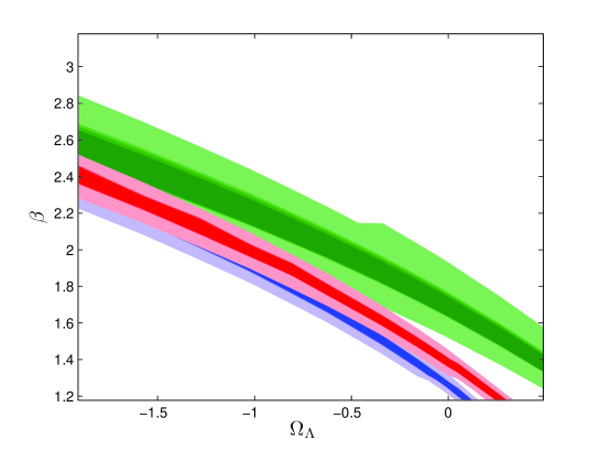
$\Omega_{\Lambda}$	$\beta\equiv r_{\mathrm{c}}H_{0}$	$\Omega_{\mathrm{m}}$	$\chi^{2}$
$-10.0$	4.70	0.29	177
$-5.0$	3.47	0.29	177
$-2.0$	2.44	0.29	177
$-1.0$	1.98	0.29	179
$-0.5$	1.71	0.28	181
0	1.38	0.28	188
0.2	1.23	0.27	197
0.5	0.99	0.29	228

Figure 4: Plot showing the one sigma (dark color) and three sigma (light color) range for best-fit values of $\beta$ for given values of $\Omega_{\Lambda}$ for CMB distance (green), SN (blue) and combined (red) For $\Omega_{\Lambda}$ close to 0 the preferred values for the two data sets are significantly different, leading to a poor overall fit. As $\Omega_{\Lambda}\rightarrow-\infty$ the preferred parameter spaces increasingly overlap. In this regime DGP is indistinguishable from GR. The table presents values of best-fit $\beta$’s for a selection of $\Omega_{\Lambda}$ and the $\chi^{2}$’s of the respective fits to combined CMB-distance and SN data. It can be clearly seen that a positive bulk cosmological constant is strongly excluded.

6.3 Simulation Results

The matter power spectrum for DGP is slightly different than that for $\Uplambda$CDM. We have found that there is excess power at large scales and a deficiency of power at low scales. Results are shown in Figures 5 and 6. This change is a result of the different late-time evolution of the gravitational potential and the change in the rate of growth of density perturbations associated with it.

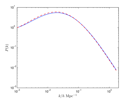
Figure 5: Comparison of dark-matter power spectra for $\Uplambda$CDM (solid line) and DGP ($\Omega_{\Lambda}=0,\beta=1.38$, dashed). The spectra have been normalized to unity at $k=10^{-3}h$ Mpc^-1. There is excess power at large scales and a power deficiency at low scales.

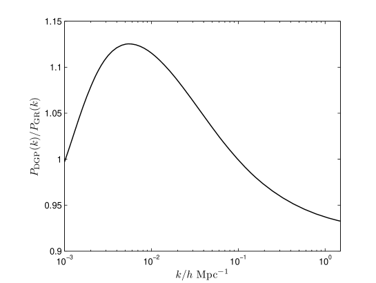
Figure 6: Ratio of dark-matter power spectra for DGP ($\Omega_{\Lambda}=0,\beta=1.38$) and $\Uplambda$CDM. Both spectra are initially normalized to unity at $k=10^{-3}h$ Mpc^-1.

Using the sets of parameters presented in Figure 4, we computed the ISW effect for the DGP model. We have found it to be significantly reduced at low multipoles and to have a (very) slight excess in the power for $\ell$ above 20 as compared to the concordance $\Uplambda$CDM model. Making the bulk cosmological more negative restores the behavior observed in $\Uplambda$CDM. A positive $\Omega_{\Lambda}$ significantly increases the ISW effect. The results are shown in Figure 7.

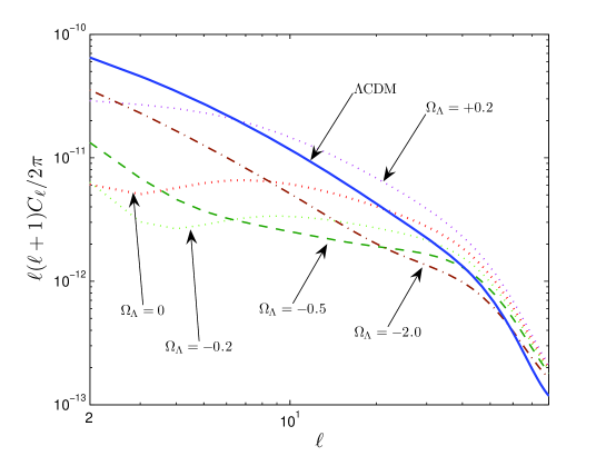
Figure 7: Contribution to $C_{\ell}$ from ISW effect as calculated for $\Uplambda$CDM and a range of DGP cosmologies. The effect is significantly reduced at low multipoles in DGP. Making the bulk cosmological constant more negative brings the effect back to $\Uplambda$CDM levels. Making $\Omega_{\Lambda}$ more negative brings the DGP power spectrum towards the $\Uplambda$CDM one.

6.4 Impact on CMB

From the fits performed in §6.2, we obtain a range of values of $\beta$ for each $\Omega_{\Lambda}$ which satisfy the constraints of the supernova data and the distance to the last-scattering surface. In our subsequent analysis and simulations we pick as $\beta$ the central values of the likelihood distributions for each $\Omega_{\Lambda}$. A selection of $\Omega_{\Lambda}$ and $\beta$ pairs is presented in the table contained in Figure 4.

By requiring that the distance to the last scattering surface is effectively fixed and by assuming the same radiation-density-to-matter-density ratio as in the concordance model, we ensure that the part of the CMB spectrum resulting from plasma oscillations remains unchanged, despite the different theory of gravity. We are thus able to take the $\Uplambda$CDM output of CMBFAST and ‘replace’ the ISW part of the power spectrum with the new DGP calculation, provided we properly take into account the cross-correlations between the ISW effect and the other contributions to the CMB power spectrum.

Since the low multipoles are dominated by the SW and ISW effects, we can compute both the ISW and SW effect in all cases and then assume that the correlation between the two is equal to the correlation between the ISW contribution and the rest of the signal. The procedure is explained in detail in Appendix B.

The results of performing the above procedure for models for DGP cosmologies with a range of $\Omega_{\Lambda}$ (with $\beta$ as implied by SNe Ia data and $d_{\text{ls}}$ as from WMAP) are presented in Figure 8. The total signal strength at low multipoles is significantly reduced. The likelihood for $\Omega_{\Lambda}$ as implied by the fit to the low-multipole WMAP data alone is presented in Figure 9. For this data alone the maximum likelihood is found at $\Omega_{\Lambda}=+0.06$, with a bulk cosmological constant higher than that strongly excluded. Thus, the CMB data alone slightly prefer pure DGP to $\Uplambda$CDM.

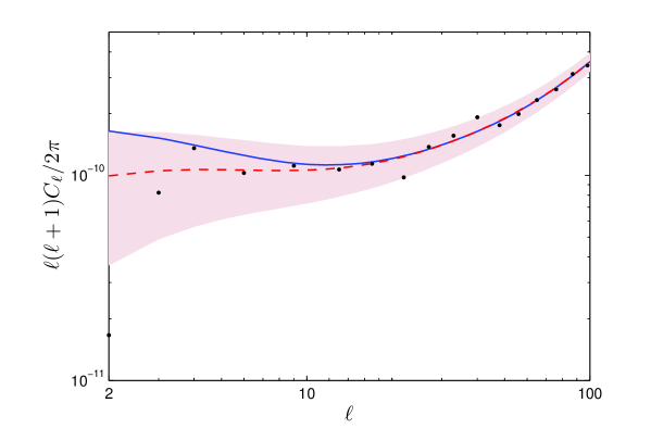
Figure 8: Output of CMBFAST for concordance $\Uplambda$CDM (blue solid line) and its modification for pure DGP ($\Omega_{\Lambda}=0$, red dashed line). Shaded are represents cosmic variance for pure DGP. WMAP measurements have been plotted in black. DGP reduces power at the lowest multipoles, bringing the power spectrum into slightly better agreement with measurement.

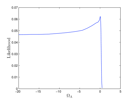
Figure 9: Likelihood for a range of values of $\Omega_{\Lambda}$ as implied solely by data from low-multipole WMAP measurements. The preferred value is $\Omega_{\Lambda}=+0.06$ with the upper half-maximum lying at lying at $+0.3$. Normalization is arbitrary.

Finally, we combine the likelihoods obtained from the SNe Ia data, and the CMB data, presented in Figure 9 to obtain an overall likelihood distribution for $\Omega_{\Lambda}$. This has been presented in Figure 10. Taking all experimental data together does not change the conclusion that $\Lambda$CDM is preferred to DGP: the better fit to low-$\ell$ multipole data of WMAP is not enough to compensate for the inconsistency between fits to CMB distance and supernova data.

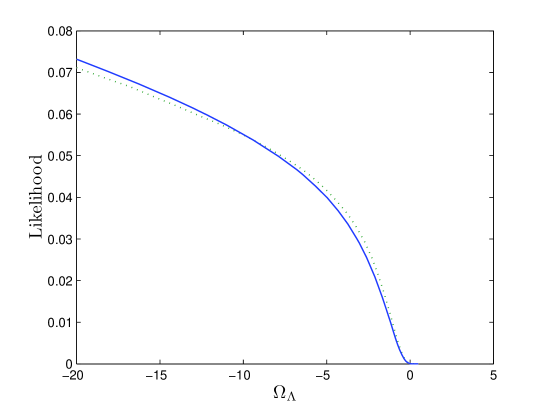
Figure 10: Likelihood for a range of values of $\Omega_{\Lambda}$ as implied by data: dotted line includes only CMB distance and SNe Ia. Solid line is the modification to the likelihood caused by adding constraints from low-multipole WMAP data. Despite the fact that WMAP data prefers pure DGP, the preferred choice for the value of the bulk cosmological constant is high enough to be excluded by the other data. $\Uplambda$CDM is clearly preferred.

7 Conclusions

We have performed a projection of the equations of the Dvali–Gabadadze–Porrati modified theory of gravity in 5D bulk (Minkowski, de Sitter and anti-de Sitter) onto a 4D brane embedded in it. We have rederived a cosmological solution to the theory and have derived equations governing the evolution of linear perturbations. We find that the theory governing the linear perturbations, in certain regimes, is one where $G$ is not a constant, but is dependent on the average energy density in the universe.

Using the new equations, we built a simple cosmological simulation containing radiation and dark matter, driven by DGP gravity. We have discovered that, in DGP cosmologies, the Newtonian potential $\Phi$ exhibits a period of growth at late times, prior to its decay; this is in contrast with GR, where the potential decays once dark energy dominates. The precise details of this effect are a function of the wavelength of the perturbation, and lead to an altered transfer function and a changed dark-matter power spectrum, with slightly higher power at large scales.

The impact of the change in the evolution of the potentials can be seen through the Integrated Sachs-Wolfe effect. We simulate the CMB anisotropy and demonstrate that in DGP cosmologies the ISW effect is significantly weaker at low multipoles.

We constrain the parameters of the theory through a fitting procedure using supernova data and the WMAP results and perform a calculation of the likelihood function for the parameter space. We find that assuming a flat cosmology, pure DGP with no bulk cosmological constant is significantly worse when simultaneously fit to supernova data and the distance to the last-scattering surface. DGP fits better to low-$\ell$ multipole data from WMAP, owing to the reduced ISW effect. However, this does not compensate for the poor fit to the former, leading to the conclusion that GR and $\Lambda$CDM are preferred by all the data available taken together.

8 Acknowledgements

We would like to thank Wayne Hu, Yong-Seon Song and Dragan Huterer for fruitful discussions. This work was supported in part by the U.S. Dept. of Energy contract DE-FG02-90ER-40560, the NSF grant PHY-0114422, and the David and Lucile Packard Foundation. The KICP is an NSF Physics Frontier Center.

Appendix A Derivation of On-Brane Field Equations

In this appendix we will replicate the work of [30, 31], deriving the projected, on-brane field equations for DGP gravity in 5D bulk.

We start off with Einstein’s equation in a 5D manifold $\mathcal{M}$

$$G_{\mu\nu}=\kappa^{2}T_{\mu\nu}\,.$$ (47)

The Greek indices run over all the dimensions, i.e. from 0 to 4.

We want to put in a 3-brane, $\mathcal{B}$, (we will denote its position by invoking a spacelike vector field $\chi$ in the neighborhood of the brane, such that $\chi=0$ will coincide with the position of the brane. We want then to find the effective equation of motion for gravity on $\mathcal{B}$ itself.

Let us first take care of the LHS of (47). We will first define the induced metric on the 3-brane, $q_{\mu\nu}$:

$$q_{\mu\nu}=g_{\mu\nu}-n_{\mu}n_{\nu}\,,$$ (48)

where $g_{\mu\nu}$ is the metric on $\mathcal{M}$, and $n^{\mu}$ is a spacelike vector field in $\mathcal{M}$, with unit norm, which is normal to the brane at $\chi=0$. Now we invoke the Gauss equation to calculate the Riemann tensor on the 3-brane

$${}^{(4)}R^{\alpha}_{\phantom{\alpha}\beta\gamma\delta}=\ ^{(5)}R^{\mu}_{\phantom{\mu}\nu\rho\sigma}q^{\alpha}_{\phantom{\alpha}\mu}q^{\nu}_{\phantom{\nu}\beta}q^{\rho}_{\phantom{\rho}\gamma}q^{\sigma}_{\phantom{\sigma}\delta}+K^{\alpha}_{\phantom{\alpha}\gamma}K_{\beta\delta}-K^{\alpha}_{\phantom{\alpha}\delta}K_{\beta\gamma}\,,$$ (49)

where $K_{\mu\nu}:=q^{\alpha}_{\phantom{\alpha}\mu}q^{\beta}_{\phantom{\beta}\nu}\nabla_{\alpha}n_{\beta}$ is the extrinsic curvature.

In order to simplify our notation, we are going to define the perpendicular subscript to signify $A_{\mu\perp}:=A_{\mu\nu}n^{\nu}$.

Contracting $\alpha$ and $\gamma$ in (49) we obtain the 4D Ricci tensor:

$${}^{(4)}R_{\beta\delta}=\ ^{(5)}R_{\nu\sigma}q^{\nu}_{\phantom{\nu}\beta}q^{\sigma}_{\phantom{\sigma}{\delta}}-\ ^{(5)}R^{\perp}_{\phantom{\perp}\nu\perp\sigma}q^{\nu}_{\phantom{\nu}\beta}q^{\sigma}_{\phantom{\sigma}\delta}+KK_{\beta\delta}-K_{\beta}^{\phantom{\beta}\alpha}K_{\delta\alpha}\,.$$ (50)

and, then, the 4D Ricci scalar:

$${}^{(4)}R:=\ ^{(4)}R_{\mu\nu}g^{\mu\nu} =\ ^{(5)}R_{\mu\nu}q^{\mu\nu}-\ ^{(5)}R^{\perp}_{\phantom{\perp}\mu\perp\nu}q^{\mu\nu}+K^{2}-K_{\mu}^{\phantom{\mu}\nu}K^{\mu}_{\phantom{\mu}\nu}$$ (51)

$$=\ ^{(5)}R-\ ^{(5)}R_{\perp\perp}-\ ^{(5)}R^{\perp\phantom{\beta\perp}\beta}_{\phantom{\perp}\beta\perp}+\ \underbrace{{}^{(5)}R^{\perp}_{\phantom{\perp}\perp\perp\perp}}_{=0}+K^{2}-K_{\alpha\beta}K^{\alpha\beta}\,.$$

An observer on the brane will only be able to measure the 4D Ricci tensor and scalar, and not their five-dimensional counterparts, so will naturally define the 4D Einstein tensor as:

$${}^{(4)}G_{\beta\delta} :=\ ^{(4)}R_{\beta\delta}-\frac{1}{2}q_{\beta\delta}\ ^{(4)}R=$$ (52)

$$=\ ^{(5)}R_{\mu\nu}q^{\mu}_{\phantom{\mu}\beta}q^{\nu}_{\phantom{\nu}\delta}-\ ^{(5)}R^{\perp}_{\phantom{\perp}\mu\perp\nu}q^{\mu}_{\phantom{\mu}\beta}q^{\nu}_{\phantom{\nu}\delta}-\frac{1}{2}g_{\mu\nu}q^{\mu}_{\phantom{\mu}\beta}q^{\nu}_{\phantom{\nu}\delta}\left({}^{(5)}R-\ ^{(5)}R_{\perp\perp}-\ ^{(5)}R^{\perp\phantom{\beta\perp}\alpha}_{\phantom{\perp}\alpha\perp}\right)$$

$$\qquad+KK_{\beta\delta}-K_{\beta}^{\phantom{\beta}\alpha}K_{\delta\alpha}-\frac{1}{2}q_{\beta\delta}\left(K^{2}-K_{\alpha\beta}K^{\alpha\beta}\right)\,.$$

We can simplify this by:

$${}^{(5)}R_{\perp\perp}=g^{\alpha\beta}n^{\gamma}\ {}^{(5)}R_{\beta\gamma\alpha\perp}=g^{\alpha\beta}n_{\gamma}\,^{(5)}R^{\gamma}_{\phantom{\gamma}\beta\perp\alpha}=\ ^{(5)}R^{\perp\phantom{\beta\perp}\beta}_{\phantom{\perp}\beta\perp}\,.$$ (53)

and also expanding the Riemann tensor in terms of the Riccis and the Weyl tensor in 5D [41, (3.2.28)]:

$$q^{\alpha}_{\phantom{\alpha}\mu}q^{\beta}_{\phantom{\alpha}\nu}n^{\rho}n^{\sigma}\ {}^{(5)}R_{\rho\alpha\sigma\beta}=q^{\alpha}_{\phantom{\alpha}\mu}q^{\beta}_{\phantom{\alpha}\nu}n^{\rho}n^{\sigma}\left(\frac{1}{3}\left(g_{\rho\sigma}\ ^{(5)}R_{\beta\alpha}-g_{\rho\beta}\ ^{(5)}R_{\sigma\alpha}-g_{\alpha\sigma}\ ^{(5)}R_{\beta\rho}+\right.\right.$$ (54)

$$\left.\left.\qquad+g_{\alpha\beta}\ ^{(5)}R_{\sigma\rho}\right)-\frac{1}{12}\left(g_{\rho\sigma}g_{\beta\alpha}-g_{\rho\beta}g_{\sigma\alpha}\right)\ ^{(5)}R+\ ^{(5)}C_{\rho\alpha\sigma\beta}\right)=$$

$$=\frac{1}{3}\left(\ {}^{(5)}R_{\alpha\beta}q^{\alpha}_{\phantom{\alpha}\mu}q^{\beta}_{\phantom{\alpha}\nu}+q_{\mu\nu}\ ^{(5)}R_{\perp\perp}\right)-\frac{1}{12}q_{\mu\nu}\ ^{(5)}R+\underbrace{\ {}^{(5)}C_{\perp\alpha\perp\beta}q^{\alpha}_{\phantom{\alpha}\mu}q^{\beta}_{\phantom{\alpha}\nu}}_{=:E_{\mu\nu}}\,.$$

We can also manipulate the 5D Einstein equation (47) to obtain:

$${}^{(5)}R =-\frac{2}{3}\kappa^{2}T$$ (55)

$${}^{(5)}R_{\rho\sigma} =\kappa^{2}\left(T_{\rho\sigma}-\frac{1}{3}g_{\rho\sigma}T\right)$$ (56)

$$R_{\perp\perp} =\kappa^{2}\left(T_{\perp\perp}-\frac{1}{3}T\right)\,.$$ (57)

Using all of the above in (52), we obtain:

$${}^{(4)}G_{\mu\nu} =\ ^{(5)}G_{\rho\sigma}q_{\mu}^{\phantom{\mu}\rho}q_{\nu}^{\phantom{\nu}\sigma}+\,^{(5)}R_{\perp\perp}q_{\mu\nu}+KK_{\mu\nu}-K_{\mu}^{\phantom{\mu}\rho}K_{\nu\rho}-\frac{1}{2}q_{\mu\nu}\left(K^{2}-K^{\alpha\beta}K_{\alpha\beta}\right)-$$

$$\qquad-\frac{1}{3}\,^{(5)}R_{\alpha\beta}q^{\alpha}_{\phantom{\alpha}\mu}q^{\beta}_{\phantom{\beta}\nu}-\frac{1}{3}q_{\mu\nu}\,^{(5)}R_{\perp\perp}+\frac{1}{12}q_{\mu\nu}\,^{(5)}R-E_{\mu\nu}=$$

$$=\frac{2\kappa^{2}}{3}\left(T_{\rho\sigma}q^{\rho}_{\phantom{\rho}\mu}q^{\sigma}_{\phantom{\sigma}\nu}+q_{\mu\nu}\left(T_{\perp\perp}-\frac{1}{4}T\right)\right)+KK_{\mu\nu}-K_{\mu}^{\phantom{\mu}\rho}K_{\nu\rho}-$$

$$\qquad-\frac{1}{2}q_{\mu\nu}\left(K^{2}-K^{\alpha\beta}K_{\alpha\beta}\right)-E_{\mu\nu}\,.$$ (58)

Now let’s take care of the energy-momentum tensor. It has contributions from the bulk (which we will limit to just a bulk cosmological constant, $\Lambda$) as well as the brane contributions. One of the contributions in the brane is the radiatively induced DGP 4-gravity term; the action here is just the usual $\mu^{-2}\delta(\chi)\int\!\mathrm{d}^{4}x\,^{(4)}R$, restricted to the brane, the variation of which gives the 4D Einstein tensor. The stress-energy tensor has the form:

$$T_{\mu\nu}=-\Lambda g_{\mu\nu}+\underbrace{\left(-\lambda q_{\mu\nu}+\tau_{\mu\nu}-\mu^{-2}\,{}^{(4)}G_{\mu\nu}\right)}_{=:S_{\mu\nu}}\delta(\chi)\,.$$ (59)

We are going to perform our calculation just off the brane. The energy-momentum tensor there consists of just the bulk cosmological constant. The extrinsic curvature can be determined from the Israel junction conditions, one of the formulations of which allows us to compute the jump in the metric and extrinsic curvature across a thin shell of non-zero momentum-energy [32]:

$$q_{\mu\nu}^{+}-q_{\mu\nu}^{-}=:[q_{\mu\nu}] =0$$ (60)

$$[K_{\mu\nu}] =-\kappa^{2}\left(S_{\mu\nu}-\frac{1}{3}q_{\mu\nu}S\right)$$ (61)

Assuming that the universe is symmetric about the brane allows us to obtain the values of the extrinsic curvature explicitly, $K_{\mu\nu}^{+}=-K_{\mu\nu}^{-}=\frac{1}{2}[K_{\mu\nu}]$ and $K^{+}=\frac{1}{6}\kappa^{2}S$. Substituting into (A) and making 4D subscripts implicit:

$$G_{\mu\nu} =-\frac{\kappa^{2}}{2}\Lambda q_{\mu\nu}-\frac{\kappa^{4}}{12}S\left(S-\frac{1}{3}q_{\mu\nu}S\right)-\frac{\kappa^{4}}{4}\left(S^{\mathchoice{\makebox[4.21783pt][c]{$\displaystyle$}}{\makebox[4.21783pt][c]{$\textstyle$}}{\makebox[2.95248pt][c]{$\scriptstyle$}}{\makebox[2.10892pt][c]{$\scriptscriptstyle$}}\leavevmode{\sigma}}_{\leavevmode{\mu}\mathchoice{\makebox[3.9999pt][c]{$\displaystyle$}}{\makebox[3.9999pt][c]{$\textstyle$}}{\makebox[2.79993pt][c]{$\scriptstyle$}}{\makebox[1.99994pt][c]{$\scriptscriptstyle$}}}-\frac{1}{3}q^{\mathchoice{\makebox[4.21783pt][c]{$\displaystyle$}}{\makebox[4.21783pt][c]{$\textstyle$}}{\makebox[2.95248pt][c]{$\scriptstyle$}}{\makebox[2.10892pt][c]{$\scriptscriptstyle$}}\leavevmode{\sigma}}_{\leavevmode{\mu}\mathchoice{\makebox[3.9999pt][c]{$\displaystyle$}}{\makebox[3.9999pt][c]{$\textstyle$}}{\makebox[2.79993pt][c]{$\scriptstyle$}}{\makebox[1.99994pt][c]{$\scriptscriptstyle$}}}S\right)\left(S_{\nu\sigma}-\frac{1}{3}q_{\nu\sigma}S\right)-$$

$$\qquad-\frac{\kappa^{4}}{8}q_{\mu\nu}\left(\frac{1}{9}S^{2}-\left(S_{\mu\nu}-\frac{1}{3}q_{\mu\nu}S\right)^{2}\right)\,.$$ (62)

We then substitute for $S_{\mu\nu}$ from its definition and, after a bit of algebra, obtain:

$$\left(1+\frac{\lambda\kappa^{4}}{6\mu^{2}}\right)G_{\mu\nu}=-\left(\frac{\kappa^{2}}{2}\Lambda+\frac{\kappa^{4}\lambda^{2}}{12}\right)q_{\mu\nu}+\frac{\lambda\kappa^{4}}{6}\tau_{\mu\nu}+\kappa^{4}\pi_{\mu\nu}+\frac{\kappa^{4}}{\mu^{4}}\gamma_{\mu\nu}+\frac{\kappa^{4}}{\mu^{2}}\xi_{\mu\nu}-E_{\mu\nu}\,.$$ (63)

where the new tensors are quadratic in $G_{\mu\nu}$ and $\tau_{\mu\nu}$ and are defined as:

$$\pi_{\mu\nu} =\frac{1}{12}\tau\tau_{\mu\nu}-\frac{1}{4}\tau^{\mathchoice{\makebox[4.21783pt][c]{$\displaystyle$}}{\makebox[4.21783pt][c]{$\textstyle$}}{\makebox[2.95248pt][c]{$\scriptstyle$}}{\makebox[2.10892pt][c]{$\scriptscriptstyle$}}\leavevmode{\alpha}}_{\leavevmode{\mu}\mathchoice{\makebox[4.4779pt][c]{$\displaystyle$}}{\makebox[4.4779pt][c]{$\textstyle$}}{\makebox[3.13454pt][c]{$\scriptstyle$}}{\makebox[2.23895pt][c]{$\scriptscriptstyle$}}}\tau_{\nu\alpha}+\frac{1}{8}q_{\mu\nu}\left(\tau_{\alpha\beta}\tau^{\alpha\beta}-\frac{1}{3}\tau^{2}\right)$$ (64)

$$\gamma_{\mu\nu} =\frac{1}{12}GG_{\mu\nu}-\frac{1}{4}G^{\mathchoice{\makebox[4.21783pt][c]{$\displaystyle$}}{\makebox[4.21783pt][c]{$\textstyle$}}{\makebox[2.95248pt][c]{$\scriptstyle$}}{\makebox[2.10892pt][c]{$\scriptscriptstyle$}}\leavevmode{\alpha}}_{\leavevmode{\mu}\mathchoice{\makebox[4.4779pt][c]{$\displaystyle$}}{\makebox[4.4779pt][c]{$\textstyle$}}{\makebox[3.13454pt][c]{$\scriptstyle$}}{\makebox[2.23895pt][c]{$\scriptscriptstyle$}}}G_{\nu\alpha}+\frac{1}{8}q_{\mu\nu}\left(G_{\alpha\beta}G^{\alpha\beta}-\frac{1}{3}G^{2}\right)$$ (65)

$$\xi_{\mu\nu} =-\frac{1}{12}\left(\tau G_{\mu\nu}+\tau_{\mu\nu}G\right)+\frac{1}{4}\left(\tau^{\mathchoice{\makebox[4.21783pt][c]{$\displaystyle$}}{\makebox[4.21783pt][c]{$\textstyle$}}{\makebox[2.95248pt][c]{$\scriptstyle$}}{\makebox[2.10892pt][c]{$\scriptscriptstyle$}}\leavevmode{\alpha}}_{\leavevmode{\mu}\mathchoice{\makebox[4.4779pt][c]{$\displaystyle$}}{\makebox[4.4779pt][c]{$\textstyle$}}{\makebox[3.13454pt][c]{$\scriptstyle$}}{\makebox[2.23895pt][c]{$\scriptscriptstyle$}}}G_{\alpha\nu}+G^{\mathchoice{\makebox[4.21783pt][c]{$\displaystyle$}}{\makebox[4.21783pt][c]{$\textstyle$}}{\makebox[2.95248pt][c]{$\scriptstyle$}}{\makebox[2.10892pt][c]{$\scriptscriptstyle$}}\leavevmode{\alpha}}_{\leavevmode{\mu}\mathchoice{\makebox[4.4779pt][c]{$\displaystyle$}}{\makebox[4.4779pt][c]{$\textstyle$}}{\makebox[3.13454pt][c]{$\scriptstyle$}}{\makebox[2.23895pt][c]{$\scriptscriptstyle$}}}\tau_{\nu\alpha}\right)-\frac{1}{4}q_{\mu\nu}\left(\tau_{\alpha\beta}G^{\alpha\beta}-\frac{1}{3}\tau G\right)$$ (66)

$$E_{\mu\nu} =C^{\leavevmode{\perp}\mathchoice{\makebox[4.4779pt][c]{$\displaystyle$}}{\makebox[4.4779pt][c]{$\textstyle$}}{\makebox[3.13454pt][c]{$\scriptstyle$}}{\makebox[2.23895pt][c]{$\scriptscriptstyle$}}\mathchoice{\makebox[5.25pt][c]{$\displaystyle$}}{\makebox[5.25pt][c]{$\textstyle$}}{\makebox[3.67499pt][c]{$\scriptstyle$}}{\makebox[2.625pt][c]{$\scriptscriptstyle$}}\mathchoice{\makebox[3.95938pt][c]{$\displaystyle$}}{\makebox[3.95938pt][c]{$\textstyle$}}{\makebox[2.77156pt][c]{$\scriptstyle$}}{\makebox[1.97969pt][c]{$\scriptscriptstyle$}}}_{\mathchoice{\makebox[5.25pt][c]{$\displaystyle$}}{\makebox[5.25pt][c]{$\textstyle$}}{\makebox[3.67499pt][c]{$\scriptstyle$}}{\makebox[2.625pt][c]{$\scriptscriptstyle$}}\leavevmode{\alpha}\leavevmode{\perp}\leavevmode{\beta}}q^{\leavevmode{\alpha}\mathchoice{\makebox[4.21783pt][c]{$\displaystyle$}}{\makebox[4.21783pt][c]{$\textstyle$}}{\makebox[2.95248pt][c]{$\scriptstyle$}}{\makebox[2.10892pt][c]{$\scriptscriptstyle$}}}_{\mathchoice{\makebox[4.4779pt][c]{$\displaystyle$}}{\makebox[4.4779pt][c]{$\textstyle$}}{\makebox[3.13454pt][c]{$\scriptstyle$}}{\makebox[2.23895pt][c]{$\scriptscriptstyle$}}\leavevmode{\mu}}q^{\leavevmode{\beta}\mathchoice{\makebox[3.45787pt][c]{$\displaystyle$}}{\makebox[3.45787pt][c]{$\textstyle$}}{\makebox[2.42052pt][c]{$\scriptstyle$}}{\makebox[1.72893pt][c]{$\scriptscriptstyle$}}}_{\mathchoice{\makebox[3.95938pt][c]{$\displaystyle$}}{\makebox[3.95938pt][c]{$\textstyle$}}{\makebox[2.77156pt][c]{$\scriptstyle$}}{\makebox[1.97969pt][c]{$\scriptscriptstyle$}}\leavevmode{\nu}}\,.$$ (67)

These quadratic tensors are related to $f_{\mu\nu}$ of (11) by

$$f_{\mu\nu}=\mu^{4}\pi_{\mu\nu}+\mu^{2}\xi_{\mu\nu}+\gamma_{\mu\nu}\,.$$ (68)

Appendix B Modifying CMBFAST data

This appendix explains how CMBFAST data was modified to reflect the expected DGP signal.

Our cosmological simulation was used to calculate the contribution to the CMB power spectrum from the ISW and SW effects, as well as the total of the two (taking into account the cross-correlation). We then defined the ISW-SW cross-correlation factor as

$$R:=\frac{C_{\ell}^{\text{ISW-SW}}}{\sqrt{C_{\ell}^{\text{ISW-ISW}}C_{\ell}^{\text{SW-SW}}}}=\frac{C_{\ell}^{\text{total}}-C_{\ell}^{\text{SW-SW}}-C_{\ell}^{\text{ISW-ISW}}}{2\sqrt{C_{\ell}^{\text{ISW-ISW}}C_{\ell}^{\text{SW-SW}}}}$$ (69)

The $R$ thus defined was then assumed to be identical to the cross-correlation factor between the ISW effect and the total CMBFAST signal. This is a very good approximation at the lowest multipoles. With this assumption we can compute the non-ISW part of the power spectrum by solving for $C_{\ell}^{\sim\text{ISW}}$ in

$$C_{\ell}^{\text{CMBFAST}}\approx C_{\ell}^{\sim\text{ISW}}+2\sqrt{C_{\ell}^{\sim{\text{ISW}}}C_{\ell}^{\text{ISW-ISW}}}R+C_{\ell}^{\text{ISW-ISW}}$$ (70)

Finally, to compute the power spectrum for DGP cosmologies, we take the values of $R$ and $C_{\ell}^{\text{ISW-ISW}}$ calculated for the particular model and use them in equation (70). This output is presented in Figure 8.

References

• [1] Supernova Search Team Collaboration, A. G. Riess et. al., Observational evidence from supernovae for an accelerating universe and a cosmological constant, Astron. J. 116 (1998) 1009–1038 [astro-ph/9805201].
• [2] Supernova Cosmology Project Collaboration, S. Perlmutter et. al., Measurements of omega and lambda from 42 high-redshift supernovae, Astrophys. J. 517 (1999) 565–586 [astro-ph/9812133].
• [3] Supernova Search Team Collaboration, J. L. Tonry et. al., Cosmological results from high-z supernovae, Astrophys. J. 594 (2003) 1–24 [astro-ph/0305008].
• [4] C. L. Bennett et. al., First year wilkinson microwave anisotropy probe (wmap) observations: Preliminary maps and basic results, Astrophys. J. Suppl. 148 (2003) 1 [astro-ph/0302207].
• [5] S. Weinberg, The cosmological constant problem, Rev. Mod. Phys. 61 (1989) 1–23.
• [6] S. M. Carroll, The cosmological constant, Living Rev. Rel. 4 (2001) 1 [astro-ph/0004075].
• [7] P. J. E. Peebles and B. Ratra, The cosmological constant and dark energy, Rev. Mod. Phys. 75 (2003) 559–606 [astro-ph/0207347].
• [8] C. Wetterich, Cosmology and the fate of dilatation symmetry, Nucl. Phys. B302 (1988) 668.
• [9] B. Ratra and P. J. E. Peebles, Cosmological consequences of a rolling homogeneous scalar field, Phys. Rev. D37 (1988) 3406.
• [10] R. R. Caldwell, R. Dave and P. J. Steinhardt, Cosmological imprint of an energy component with general equation-of-state, Phys. Rev. Lett. 80 (1998) 1582–1585 [astro-ph/9708069].
• [11] C. Armendariz-Picon, T. Damour and V. Mukhanov, k-inflation, Phys. Lett. B458 (1999) 209–218 [hep-th/9904075].
• [12] C. Armendariz-Picon, V. Mukhanov and P. J. Steinhardt, A dynamical solution to the problem of a small cosmological constant and late-time cosmic acceleration, Phys. Rev. Lett. 85 (2000) 4438–4441 [astro-ph/0004134].
• [13] C. Armendariz-Picon, V. Mukhanov and P. J. Steinhardt, Essentials of k-essence, Phys. Rev. D63 (2001) 103510 [astro-ph/0006373].
• [14] L. Mersini, M. Bastero-Gil and P. Kanti, Relic dark energy from trans-planckian regime, Phys. Rev. D64 (2001) 043508 [hep-ph/0101210].
• [15] R. R. Caldwell, A phantom menace?, Phys. Lett. B545 (2002) 23–29 [astro-ph/9908168].
• [16] S. M. Carroll, M. Hoffman and M. Trodden, Can the dark energy equation-of-state parameter w be less than -1?, Phys. Rev. D68 (2003) 023509 [astro-ph/0301273].
• [17] V. Sahni and A. A. Starobinsky, The case for a positive cosmological lambda-term, Int. J. Mod. Phys. D9 (2000) 373–444 [astro-ph/9904398].
• [18] L. Parker and A. Raval, Non-perturbative effects of vacuum energy on the recent expansion of the universe, Phys. Rev. D60 (1999) 063512 [gr-qc/9905031].
• [19] K. Freese and M. Lewis, Cardassian expansion: a model in which the universe is flat, matter dominated, and accelerating, Phys. Lett. B540 (2002) 1–8 [astro-ph/0201229].
• [20] G. Dvali and M. S. Turner, Dark energy as a modification of the friedmann equation, astro-ph/0301510.
• [21] S. M. Carroll, V. Duvvuri, M. Trodden and M. S. Turner, Is cosmic speed-up due to new gravitational physics?, Phys. Rev. D70 (2004) 043528 [astro-ph/0306438].
• [22] G. R. Dvali, G. Gabadadze and M. Porrati, 4d gravity on a brane in 5d minkowski space, Phys. Lett. B485 (2000) 208–214 [hep-th/0005016].
• [23] G. R. Dvali, G. Gabadadze, M. Kolanovic and F. Nitti, The power of brane-induced gravity, Phys. Rev. D64 (2001) 084004 [hep-ph/0102216].
• [24] G. R. Dvali, G. Gabadadze, M. Kolanovic and F. Nitti, Scales of gravity, Phys. Rev. D65 (2002) 024031 [hep-th/0106058].
• [25] C. Deffayet, Cosmology on a brane in minkowski bulk, Phys. Lett. B502 (2001) 199–208 [hep-th/0010186].
• [26] A. Lue, R. Scoccimarro and G. D. Starkman, Probing newton’s constant on vast scales: Dgp gravity, cosmic acceleration and large scale structure, Phys. Rev. D69 (2004) 124015 [astro-ph/0401515].
• [27] M. Ishak, A. Upadhye and D. N. Spergel, Is cosmic acceleration a symptom of the breakdown of general relativity?, astro-ph/0507184.
• [28] A. de Oliveira-Costa, M. Tegmark, M. Zaldarriaga and A. Hamilton, The significance of the largest scale cmb fluctuations in wmap, Phys. Rev. D69 (2004) 063516 [astro-ph/0307282].
• [29] G. Efstathiou, A maximum likelihood analysis of the low cmb multipoles from wmap, Mon. Not. Roy. Astron. Soc. 348 (2004) 885 [astro-ph/0310207].
• [30] T. Shiromizu, K.-i. Maeda and M. Sasaki, The einstein equations on the 3-brane world, Phys. Rev. D62 (2000) 024012 [gr-qc/9910076].
• [31] K.-i. Maeda, S. Mizuno and T. Torii, Effective gravitational equations on brane world with induced gravity, Phys. Rev. D68 (2003) 024033 [gr-qc/0303039].
• [32] W. Israel, Singular hypersurfaces and thin shells in general relativity, Nuovo Cim. B44S10 (1966) 1.
• [33] G. Gabadadze and A. Iglesias, Schwarzschild solution in brane induced gravity, hep-th/0407049.
• [34] G. Gabadadze and A. Iglesias, Short distance non-perturbative effects of large distance modified gravity, hep-th/0508201.
• [35] R. Maartens, Brane-world gravity, Living Rev. Rel. 7 (2004) 1–99 [gr-qc/0312059].
• [36] H. Collins and B. Holdom, Brane cosmologies without orbifolds, Phys. Rev. D62 (2000) 105009 [hep-ph/0003173].
• [37] Y. V. Shtanov, Closed equations on a brane, Phys. Lett. B541 (2002) 177–182 [hep-ph/0108153].
• [38] S. M. Carroll and E. A. Lim, Lorentz-violating vector fields slow the universe down, Phys. Rev. D70 (2004) 123525 [hep-th/0407149].
• [39] G. Dvali, A. Gruzinov and M. Zaldarriaga, The accelerated universe and the moon, Phys. Rev. D68 (2003) 024012 [hep-ph/0212069].
• [40] Supernova Search Team Collaboration, A. G. Riess et. al., Type ia supernova discoveries at z>1 from the hubble space telescope: Evidence for past deceleration and constraints on dark energy evolution, Astrophys. J. 607 (2004) 665–687 [astro-ph/0402512].
• [41] R. M. Wald, General Relativity. Chicago University Press, 1984.