SHELS: The Hectospec Lensing Survey

Abstract

The Smithsonian Hectospec Lensing Survey (SHELS) combines a 10,000 galaxy deep complete redshift survey with a weak lensing map from the Deep Lens Survey (Wittman et al. 2002; 2005). We use maps of the velocity dispersion based on systems identified in the redshift survey to compare the three-dimensional matter distribution with the two-dimensional projection mapped by weak lensing. We demonstrate directly that the lensing map images the three-dimensional matter distribution obtained from the kinematic data.

1 Introduction

Weak gravitational lensing maps are a powerful modern tool for probing the distribution of matter in the universe. Demonstrations of the power of weak lensing include measurements of the masses of galaxies and galaxy groups (Dell’Antonio & Tyson 1996; Hudson et al. 1998; Fischer et al. 2000; Hoekstra et al. 2003; Sheldon et al. 2004; Parker et al. 2005), maps of the mass distribution in rich clusters of galaxies (Tyson et al. 1990; Squires et al. 1996; Luppino & Kaiser 1997; Hoekstra et al. 1998; Clowe & Schneider 2001; Sheldon et al. 2001; Irgens et al. 2002; Gray et al. 2002; Wittman et al. 2003; Jee et al. 2005; Margoniner et al. 2005; Cypriano et al. 2005) and statistical detection of the lensing signal of the large-scale structure of the universe (Bacon et al. 2000; Wittman et al. 2000; Wilson et al. 2001; Bernardeau et al. 2002; Hoekstra et al. 2002; Jarvis et al. 2003; Refregier 2003; Heymans et al. 2004; van Waerbeke et al. 2005). Recently wide-field imagers on large telescopes have enabled lensing surveys of substantial objectively chosen regions where broader investigations of mass distributions in the universe can be accomplished (Kaiser 1998; Wilson et al. 2001; Brown et al. 2003). Schneider (2005) reviews the impressive recent progress in this area.

The Deep Lens Survey (Wittman et al. 2002, 2005; DLS hereafter), covers 20 square degrees in five separate four-square-degree regions. A weak lensing (convergence) map of one of the fields at (09:19:32.4 +30:00:00 (J2000)) is complete (Wittman et al. 2005). In the DLS field, distortions of resolved objects with $21<R<24.2$ reveal the matter distribution generally marked by galaxies with $R<21$, the range accessible with Hectospec (Fabricant et al. 2005), a 300-fiber moderate resolution spectrograph mounted at the $f/5$ focus of the 6.5-meter MMT.

We report initial results of combining the DLS with SHELS (Smithsonian Hectospec Lensing Survey). We explore the power of coupling a foreground redshift survey with a weak lensing map in uncovering the three-dimensional matter distribution in the universe from the scale of individual galaxies to the large-scale structure itself. In this first paper we examine the relationship between a weak lensing (convergence) map of the complete 9-hour DLS field with a “velocity dispersion” map of the same field derived from a $\sim$10,000 galaxy redshift survey to a limiting $R<20.3$. There is a striking correspondence between the lensing map and the large-scale structure revealed by the redshift survey in the redshift range $0.07<z<0.47$. The match between these assays of the matter distribution shows the broad potential power of combining these two modern tools of astrophysics.

We begin by describing the observational approaches to the lensing map (Section 2) and the Hectospec redshift survey (Section 3). In Section 4 we review the construction of the “velocity dispersion map” from the redshift survey. We cross-correlate the two maps and demonstrate that the lensing map provides a view of the matter distribution associated with large-scale structure in the range covered by the Hectospec redshift survey. We summarize in Section 5.

2 The DLS: The Deep Lens Survey Weak Lensing Map

The DLS (Wittman et al. 2002; 2005) is an NOAO Survey Project using the Mosaic I and II cameras on the 4m telescopes on Kitt Peak and Cerro Tololo. The effective exposure time of the survey is about 14500 seconds in R and the 1 $\sigma$ surface brightness limit in R is 28.7 magnitudes per square arcsecond, yielding about 45 resolved sources per square arcminute.

The DLS observing procedures described in Wittman et al. (2002, 2005) produce 40${}^{\prime}\times 40^{\prime}$ subfields of uniform image quality. To optimize the number of sources usable for construction of the weak lensing map, the R-band observations are all made in seeing better than 0.9^′′.

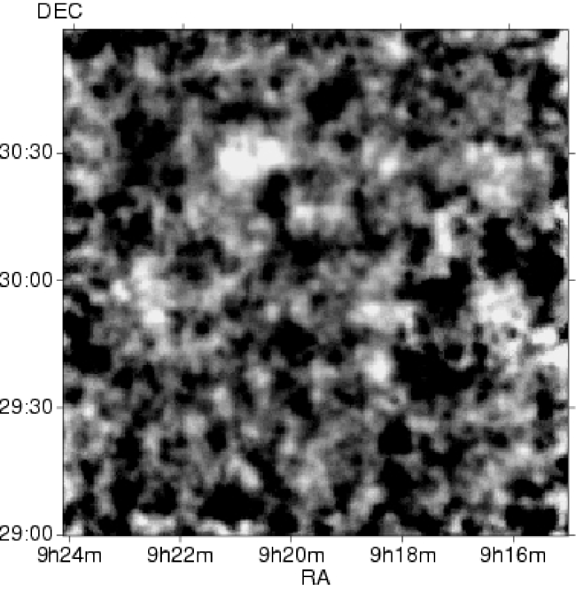
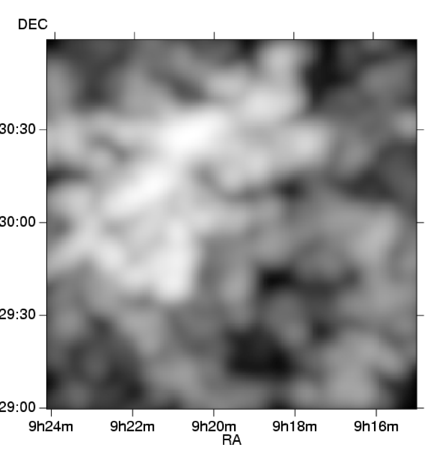
Figure 1: Convergence map for the DLS field centered at 09:19:32.4 +30:00:00 (left). The $\sigma^{2}$ map covering the redshift range 0.13-0.47 (right). The range of $\kappa$ is 0 — 0.024; the range of $\sigma$ is $0-{800}$ km s^-1. In both images 0 is black; the peak value is white.

The convergence map we construct for the DLS field centered at 09:19:32.4 +30:00:00 (Figure 1a) is somewhat shallower than the map of this field discussed by Wittman et al. (2005). Our convergence map is based on all resolved objects (size at least 1.3 times the local PSF) with R band aperture magnitude (within a 5^′′ diameter aperture) between 21 and 24.2, smaller than 8″ (to exclude nearby LSB galaxies), and well-measured (c.f. Bernstein & Jarvis 2002). Approximately $2\times 10^{5}$ galaxies contribute to the map. We used a Hectospec deep field covering the range 21 $<{\rm R}<22.5$ (Fabricant et al. 2005) to estimate the weighted mean redshift of the sources which lies between 0.60 and 0.85.

The convergence map is a direct reconstruction (Kaiser & Squires 1993) following the procedure of Fischer & Tyson (1997). We convert the measured shear into a measurement of the convergence at position ${\bf x}$ with a weight function introduced to prevent noise divergences:

$$\kappa({\bf x})={\Sigma({\bf x})\over\Sigma_{crit}}={1\over N\pi}\sum_{g}{W(|{\bf x_{g}-x}|){{e_{T}\bf(x_{g}-x)}\over|{\bf x_{g}-x}|^{2}}}$$

where $e_{T}\bf(x_{g}-x)$ is the projection of the (seeing-corrected) ellipticity tangent to the vector connecting ${\bf x}$ and ${\bf x_{g}}$, the position of source ${\bf g}$, and $W(x)=(1-e^{-x^{2}/(2r_{i}^{2})})e^{-x^{2}/(2r_{o}^{2})}$ and $r_{i}$ and $r_{o}$ are inner and outer cutoffs to the summation. We used $r_{i}=3$′ and $r_{o}=30$′. The choice of inner cutoff radii and the source density determine the final resolution of the map, $\sim$ 2.5′

3 SHELS: The Hectospec Redshift Survey

Our goal is to understand the relationship between the convergence map (Figure 1a) and the distribution of matter marked by foreground galaxies. As a first step toward that goal we used the Hectospec (Fabricant et al. 1998; Fabricant et al. 2005), a 300-fiber moderate resolution spectrograph mounted at the f/5 focus of the MMT to carry out a redshift survey of the region.

We constructed a galaxy catalog from the R-band source list for the field. We separated galaxies from stars by central surface brightness and then selected galaxies with $R<20.3$. The Hectospec positioning software (Roll et al. 1998) enables optimization of the target list to obtain an essentially complete magnitude limited survey. Our 46 Hectospec pointings in the DLS field yield reliable redshifts for 9792 galaxies with a median redshift $z=0.297$.

The Hectospec spectra cover the wavelength range $\lambda 3500-10,000$ Å with a resolution of$\sim 6$ Å. The Hectospec exposures times are 0.75 - 1.0 hours. We reduce the data using the standard Hectospec pipeline (Mink et al. 2005). We derive redshifts by application of RVSAO (Kurtz & Mink 1998) with templates constructed for this purpose (Fabricant et al. 2005). Repeat observations of 343 galaxies imply a mean external error in the redshifts of 45 km s^-1 for absorption-line galaxies and 30 km s^-1 for emission line galaxies.

The redshift survey is 95% complete for $R<19.7$. The differential completeness is 65% in the range R = 19.7-20.3. Throughout the apparent magnitude range, the redshift survey completeness is uniform over the entire DLS field.

4 A Lensing Map … A Redshift Survey

Here we examine the correspondence between the large-scale structure revealed by the redshift survey and the structure in the lensing map. The lensing map shows a complex of three overlapping peaks, DLSCL J0920.1+3029, corresponding to three extended cluster x-ray sources (Wittman et al. 2005). The Hectospec redshift survey identifies three clusters coincident with the x-ray clusters and with the convergence map peaks. CXOU J092026+302938 (Abell 781, A hereafter) has a mean redshift 0.302 and a rest frame line-of-sight velocity dispersion $\sigma_{A}$ = 674${}^{+43}_{-52}$ km s^-1 (163 members). CXOU J092053+302800 (B hereafter) has a mean redshift 0.291 and $\sigma_{B}$ = 741${}^{+35}_{-40}$ km s^-1 (123 members). Figure 2 shows the complex structure in the redshift survey in the range of these two systems; they are separate clusters, not subclumps of a single system. CXOU J092110+302751, although very close to the other two clusters on the sky, has a mean redshift of 0.427 and a velocity dispersion of 733${}^{+77}_{-112}$ km s^-1 (33 members).

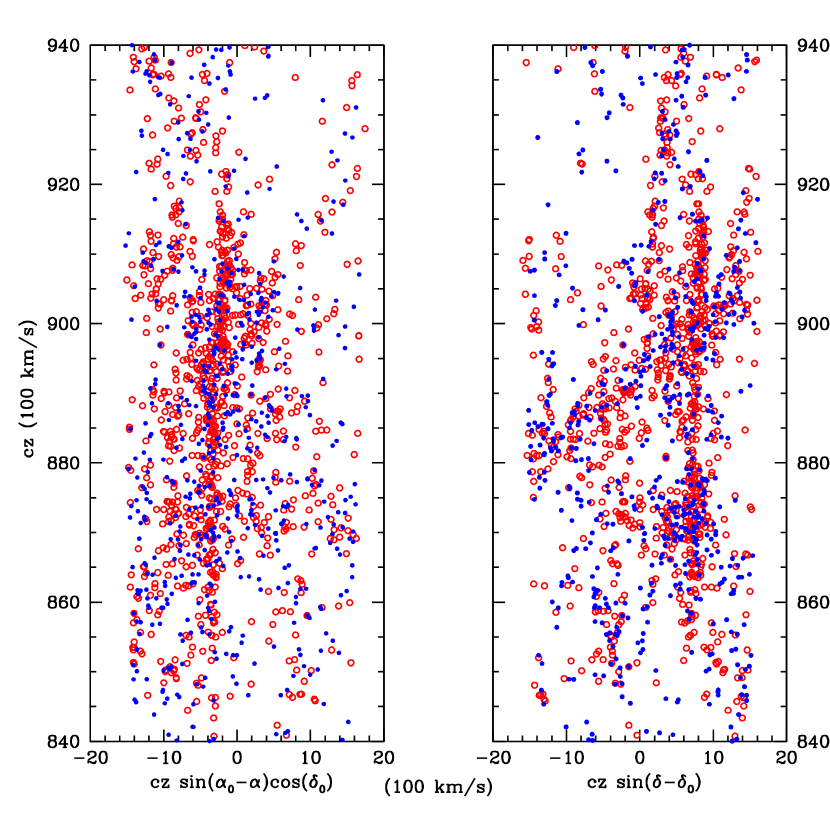
Figure 2: Section of the redshift survey including A781. Open (red) circles denote absorption-line galaxies; filled (blue) circles denote emission-line galaxies. There are 1590 galaxies in the plot. The left panel is a projection of the full declination range in right ascension; the right is a projection in declination.

Clusters A and B are the two highest amplitude peaks in the convergence map. The ratio of convergence peak amplitudes, ${p_{A}/p_{B}}=1.02\pm 0.10$, is consistent with the ratio of ${\sigma_{A}^{2}/\sigma_{B}^{2}}=0.83\pm 0.07$. In this comparison, we do not attempt to account for the superposition of the outer regions of the cluster mass distributions.

In addition to these clusters, the lensing map shows structure at lower amplitude throughout the field. We might expect to see corresponding foreground large-scale structure marked by groups of galaxies (Vale & White 2003). To identify these potentially corresponding foreground condensations, we apply a friends-of friends groups finding algorithm to the redshift survey. The algorithm we use scales the linking length to account for the variation in the observed density of a magnitude limited survey as a function of redshift (Ramella, Pisani & Geller 1997). The maps we construct are stable for density contrasts in the range 300-1200; we use maps from two catalogs of condensations with number density contrast 400 and 600 in the redshift range 0.07-0.47. The fiducial line-of-sight linking length is 180 km s^-1. At these substantial contrasts the results are robust and they are insensitive to incompleteness in the survey in the sense that we may miss real condensations but the ones we identify provide a stable estimate of the local velocity dispersion. The condensations lying closest to peaks in the lensing map all have at least 5 members.

The groups we identify in the Hectospec redshift survey range in velocity dispersion from$\sim{100}$ km s^-1 to $\sim$800 km s^-1. These systems contain $\sim{40}$% of the galaxies in the redshift survey. We use the ensemble of members of these systems to construct an approximate projected mass density map to compare with the lensing map. We divide the DLS field into a uniform 100 $\times$ 100 1.2^′ grid. At each density contrast we run through the list of group members and assign the square of the velocity dispersion, $\sigma^{2}$, of its parent group to the nearest node of the grid. If members of different groups are assigned to the same node, we assign the maximum group $\sigma^{2}$ to the node. We then have two lists (planes) of nodes and tags, one for each of the two number density contrasts. We sum the two planes and smooth the resultant map with a 2 pixel (2.4^′) Gaussian.

Figure 1b shows the $\sigma^{2}$ map covering the redshift range 0.13-0.47. The appearance of Figure 1b is insensitive to reasonable variations in the linking parameters, the group finding algorithm, or details of the construction method. The similarity between Figure 1b and the lensing map in Figure 1a is striking even discounting the A781 complex. There are some differences in both directions. There are significant lensing peaks which have no counterpart in the redshift survey. Within the sensitive range of the lensing survey, there are also dense, well-populated systems in the redshift survey which have no counterpart in the lensing map. Ramella et al. (2005, in preparation) report on the detailed match of individual systems and convergence peaks.

Figure 3: Cross-correlation of $\sigma^{2}$ maps with the convergence map (Figure 1a). The figure inidicates the $cz$ range for each $\sigma^{2}$ map.

Figure 3 shows the azimuthally averaged cross-correlation of the convergence and $\sigma^{2}$ maps in Figures 1a and 1b, respectively. We perform the image correlations by wrapping the reference image, top to bottom and left to right, equivalent to the surface of a torus; this approach preserves the proper off-peak noise behavior. The cross correlation is significant at the 6.7$\sigma_{XC}$ level where $\sigma_{XC}$ is the noise in the cross-correlation at zero lag. We evaluate $\sigma_{XC}$ by cross-correlating the $\sigma^{2}$ map with 170 noise maps. We construct noise maps by randomly assigning the j-th galaxy’s shape and orientation to the i-th galaxy coordinate. This procedure preserves the spatial sampling of the lensing map but wipes out the expected tangential ellipticity signal, and should result in a map with the same noise properties as the original map but none of the signal. The mean cross-correlation between any $\sigma^{2}$ map and the noise maps is consistent with zero; the variance in the noise map cross-correlation at zero lag, essentially the same for all of the $\sigma^{2}$ maps, is our estimate of $\sigma_{XC}$.

Figure 3 also shows the azimuthally averaged cross-correlation between the convergence and $\sigma^{2}$ maps of 6 slices each covering the redshift range $\Delta(z)=0.067$. Taken together the 6 slices cover $z=0.06-0.47$ (they are numbered sequentially (1)-(6) from low to high $z$ in Figure 3). We construct these redshift slice maps with the same method used for the map in Figure 1b. Two rich clusters (Figure 2) lie in slice (4) which returns the largest amplitude cross-correlation among the 6 slices. The clusters and several rich groups associated with subsidiary peaks in the lensing map lie in an extensive sheet-like structure which runs diagonally across the region and contributes much of the high amplitude structure in Figure 1b.

The cluster CXOU J092110+302751 at $z=0.427$ lies within slice (6) which has a cross-correlation amplitude of 4.9 $\sigma_{XC}$. The cross-correlation signal may be enhanced by superposition: the outer regions of clusters in slice (4) overlap CXOU J092110+302751 and groups surrounding the cluster are superposed on systems in the lower redshift slice (4).

Slices (2) and (5) contain no systems with $\sigma>500$ km s^-1 and yet the cross-correlation is significant. The signal comes from the large-scale structure marked by groups of galaxies; in both slices the several systems which contribute the most signal have velocity dispersions in the range 400-500 km s^-1. For slice (2) the structure in both the convergence and sigma maps is in the area 9:15:10.1 $<\alpha_{2000}<$ 9:17:04.5 and 29:00:53 $<\delta_{2000}<$ 30:01:26 ; for slice (5) it is in the range 9:14:50.9 $<\alpha_{2000}<$ 9:18:22.7 and 29:44:25 $<\delta_{2000}<$ 30:43:09. These slices demonstrate that the convergence map images the large-scale structure marked by groups.

Slice (3) provides further insight into the relationship between the foreground large-scale structure and the convergence map. The redshift range of slice (3) contains several large voids. Most of the groups in this redshift range have low velocity dispersions; the slice contains only one system with a velocity dispersion of $\sim$400 km s^-1 along with several in the 250-300 km s^-1 range. The cross-correlation amplitude is not significant as might be expected from the nature of the large-scale structure in the slice.

Slice (1) with a median $z=0.1$ provides an interesting test of the impact of lensing efficiency on the cross-correlation signal. The slice contains a cluster at $z\sim{0.12}$ with a velocity dispersion of $\sim{740}$ km s^-1, very similar to our x-ray clusters at $z=0.3-0.4$. The amplitude of the cross-correlation is only $2.6\sigma_{XC}$. The ratio of lensing efficiencies for similar systems at $z=0.1$ and $z=0.3$ is ${0.65\pm 0.06}$ for the DLS sources, probably accounting for the low cross-correlation amplitude.

Figure 3 is a direct demonstration that weak lensing images the foreground large-scale structure throughout the redshift range 0.13 — 0.47. The lensing signal is strongly modulated by the details of the three-dimensional matter distribution. At redshifts $<0.13$ we observe a decline in lensing effectiveness.

5 Conclusions

SHELS combines the power of a deep complete 10,000-galaxy redshift survey with weak lensing maps from the DLS to examine the three-dimensional matter distribution in the universe over the redshift range 0.07-0.47. We use $\sigma^{2}$ maps based on the objective identification of groups and clusters in the redshift survey as a proxy for the matter distribution in narrow redshift slices. Cross-correlation of these $\sigma^{2}$ maps with the DLS weak lensing map demonstrates that weak lensing images the foreground large-scale structure marked by groups with velocity dispersions as low as 400 km s^-1. The lensing signal is modulated by the large-scale structure and by the expected lensing efficiency.

We are extending SHELS to greater redshift in the region discussed here. We are also carrying out a similarly dense and deep redshift survey of a second DLS field. We soon plan to report in detail on further insights gained by combining deep dense redshift surveys with weak lensing convergence maps.

References

- (1) Bacon, D. J., Refregier, A. R.& Ellis, R. S. 2000, MNRAS, 318, 625
- (2) Bernardeau, F., Mellier, Y. &van Waerbeke, L., 2002, A&A, 389, L28
- (3) Bernstein G. M. & Jarvis, M. 2002, AJ, 123, 583
- (4) Brown, M. L. et al. 2003, MNRAS, 341, 100
- (5) Clowe, D.& Schneider, P. 2001, A&A, 379, 384
- (6) Cypriano, E. S. et al. 2004, ApJ, 613, 95
- (7) Dell’Antonio, I.P & Tyson, J.A. 1996, ApJ, 473, L17
- (8) Fabricant, D.G. et al. 1998, Proc. SPIE, 3355, 285
- (9) Fabricant, D.G. et al. 2005, astro-ph/0508554
- (10) Fischer, P. & Tyson, J.A. 1997, AJ, 114, 14
- (11) Gray, M. E. et al. 2002, ApJ, 568, 141
- (12) Heymans, C. et al. 2004, MNRAS, 347, 895
- (13) Hoekstra, H. et al. 1998, ApJ, 504, 636
- (14) Hoekstra, H. Yee, H. K. C. & Gladders, M. D. 2002, ApJ, 577, 595
- (15) Hoekstra, H. et al. 2003, MNRAS, 340, 609
- (16) Hudson, M. J. et al. 1998, ApJ, 503, 531
- (17) Irgens, R. J.a et al. 2002, ApJ, 579, 227
- (18) Jarvis, M. et al. 2003, AJ, 125, 1014
- (19) Jee, M. J. et al. 2005, ApJ, 618, 46
- (20) Kaiser, N. 1998, ApJ, 498, 26
- (21) Kaiser, N. and Squires, 1993, ApJ, 404, 441
- (22) Kurtz, M. J. & Mink, D. J. 1998, PASP, 110, 934
- (23) Luppino, G. A. & Kaiser, N. 1997 ApJ, 475, 20
- (24) Margoniner, V. E. et al. 2005, AJ, 129, 20
- (25) Mink, D. et al. 2005, ASP Conf. Ser., in press.
- (26) Parker,L.C., Hudson, M.J., Carlberg, R.G. & Hoekstra, H 2005, astro-ph/0508328
- (27) Ramella, M., Pisani, A. & Geller, M.J. 1997, AJ, 113, 483
- (28) Refregier, A. 2003, ARA&A, 41, 645
- (29) Roll, J. B., Fabricant, D. G.; McLeod, B. A. 1998, Proc. SPIE, 3355, 324
- (30) Schneider, P. 2005, astro-ph/0509252
- (31) Sheldon, E.S. et al. 2004, AJ, 127, 2544
- (32) Squires, G. et al. 1996, ApJ, 469, 73
- (33) Tyson, J. A., Wenk, R. A. & Valdes, F. 1990, ApJ, 349, L1
- (34) Vale, C. & White, M. 2003, ApJ, 592, 699
- (35) van Waerbeke, L., Mellier, Y. & Hoekstra, H. 2005, A&A, 429, 75
- (36) Wilson, G., Kaiser, N, & Luppino, G. A. 2001, ApJ, 556, 601
- (37) Wittman, D. M. et al. 2000, Nature, 405, 143
- (38) Wittman, D.M. et al. 200 Proc. SPIE, 4836, 73
- (39) Wittman, D.M. et al. 2003, ApJ, 597, 218
- (40) Wittman, D.M. et al. 2005, astro-ph/0507606