Ly-$\alpha$ Radiative Transfer in Cosmological Simulations and application to a $z\simeq 8$ Ly-$\alpha$ Emitter

Abstract

We develop a Ly-$\alpha$ radiative transfer (RT) Monte Carlo code for cosmological simulations. High resolution, along with appropriately treated cooling, can result in simulated environments with very high optical depths. Thus, solving the Ly-$\alpha$ RT problem in cosmological simulations can take an unrealistically long time. For this reason, we develop methods to speed up the Ly-$\alpha$ RT. With these accelerating methods, along with the parallelization of the code, we make the problem of Ly-$\alpha$ RT in the complex environments of cosmological simulations tractable. We test the RT code against simple Ly-$\alpha$ emitter models, and then we apply it to the brightest Ly-$\alpha$ emitter of a gasdynamics+N-body Adaptive Refinement Tree (ART) simulation at $z\simeq 8$. We find that recombination rather than cooling radiation Ly-$\alpha$ photons is the dominant contribution to the intrinsic Ly-$\alpha$ luminosity of the emitter, which is $\simeq 4.8\times 10^{43}$ ergs/s. The size of the emitter is pretty small, making it unresolved for currently available instruments. Its spectrum before adding the Ly-$\alpha$ Gunn-Peterson absorption (GP) resembles that of static media, despite some net inward radial peculiar motion. This is because for such high optical depths as those in ART simulations, velocities of order some hundreds km/s are not important. We add the GP in two ways. First we assume no damping wing, corresponding to the situation where the emitter lies within the HII region of a very bright quasar, and second we allow for the damping wing. Including the damping wing leads to a maximum line brightness suppression by roughly a factor of $\sim 62$. The line fluxes, even though quite faint for current ground-based telescopes, should be within reach for JWST.

draft version;

1 Introduction

Since the classic paper by Partridge & Peebles (1967), intense observational efforts have focused on the search for Ly-$\alpha$ emitters at high redshifts. Although most of the early attempts ended in negative results before the mid 1990s, recent observational advances enabled us to identify star forming galaxies at ever increasing redshifts. Currently, several observational projects, such as LALA (e.g., Rhoads et al., 2003), CADIS (e.g., Maier, 2002), the Subaru Deep Field Project (e.g., Taniguchi et al., 2005), etc., spectroscopic surveys that use lensing magnification from clusters (e.g., Santos et al., 2003), surveys that combine Subaru (e.g., Hu et al., 2004) or HST/ACS/NICMOS imaging (e.g., Stanway et al., 2004; Dickinson et al., 2004, for the GOODS survey) with Keck spectroscopy, etc., focus on finding high-z starforming galaxies. Surveys currently reach up to $z\simeq 7-8$ (e.g., see Bouwens et al., 2004, for recent results from the NICMOS observations of the HUDF) and will likely reach higher redshifts in the coming years (e.g., via JWST).

The hydrogen Ly-$\alpha$ line is a very promising way to probe the high-redshift universe. Besides yielding redshifts, the shape, equivalent width and offset of the Ly-$\alpha$ line from other emission/absorption lines potentially convey valuable information about the geometry, kinematics, and underlying stellar population of the host galaxy. Furthermore, after escaping the environment of the host galaxy, Ly-$\alpha$ photons are scattered in the surrounding IGM. The presence or absence of observed Ly-$\alpha$ emission can be used to place constraints on the state of the IGM, useful in constraining for example the epoch and topology of reionization. Because of the numerous factors that contribute to the final Ly-$\alpha$ emission, the interpretation of such features can be very complex. To use all the currently available and future observations in the most effective way possible we need to improve our theoretical understanding of Ly-$\alpha$ emission from high-redshift objects. To this end we develop a general Ly-$\alpha$ radiative transfer (RT) scheme for cosmological simulations. As an example, we apply the RT scheme to gasdynamics+N-body Adaptive Refinement Tree (ART; Kravtsov, 2003) simulations of galaxy formation.

There are quite a few studies of Ly-$\alpha$ emission from high-z objects (e.g., Gould & Weinberg, 1996; Haiman & Spaans, 1999; Loeb & Rybicki, 1999; Ahn et al., 2001, 2002; Zheng & Miralda-Escudé, 2002; Santos, 2004; Dijkstra et al., 2005a, b). The problem these studies address is highly complex and has many unknowns. Inevitably, most of these studies had to make at some point some simplifying assumptions. Usually, a high degree of symmetry for the emitting source, and its density, temperature, and velocity field is assumed. The same is the case with respect to the processes that are responsible for the production of Ly-$\alpha$ photons. On the other hand, cosmological simulations hopefully capture most of the basic elements, lifting thus practical constraints that existed in these previous studies.

There is a small number of related studies using cosmological simulations (Fardal et al., 2001; Furlanetto et al., 2003; Barton et al., 2004; Furlanetto et al., 2005; Cantalupo et al., 2005; Delliou et al., 2005a, b). Some of these simulations are lacking crucial processes such as radiative cooling of the gas and consistent RT, the various sources of Ly-$\alpha$ photons, and/or sufficient resolution in order to resolve the clumpiness of the gas. Furthermore, most of these studies do not perform Ly-$\alpha$ RT, but rather they assume that the observer sees whatever is being emitted initially, simply modified by $e^{-\tau}$ with $\tau$ the optical depth for Ly-$\alpha$ scattering due to neutral hydrogen between the emission point and the observer. Namely, in most cases Ly-$\alpha$ spectra from simulations are treated as absorption spectra when, in reality, they are scattering spectra (see, e.g., Gnedin & Prada, 2004). For gas well outside the source of emission this is an appropriate approximation since scattering off the direction of viewing removes the photons that could be observed and thus appears as effective absorption. This is no longer true for the source of emission itself, since photons that were originally emitted in directions different from the direction of observation may scatter into this direction.

It is important that the difficulty of implementing a Ly-$\alpha$ RT scheme for cosmological simulations become clear. The classical problem of resonance RT, relevant to a wide range of applications from planetary atmospheres to accretion disks, has been quite extensively studied in the literature (e.g., Zanstra, 1949; Hummer, 1962; Auer, 1968; Avery & House, 1968; Adams, 1972; Harrington, 1973; Neufeld, 1990; Ahn et al., 2001, 2002). However, analytical solutions derived in the past are applicable only to certain specific conditions. On the other hand, the slow convergence of the numerical techniques used limited the numerical studies at optical thicknesses that are relatively low compared to those encountered in high-redshift galaxies (and cosmological simulations of high-redshift galaxies, as we will show). Thus, unlike previous studies, most of which focused on the classical problem of resonant RT in a semi-infinite slab, in cosmological simulations one has to solve simultaneously thousands or even millions of these problems.Furthermore, having in mind existing and future cosmological simulations that can achieve sufficiently high resolution to resolve the gas clumpiness and that treat cooling appropriately, we anticipate column densities that are orders of magnitude higher than those found in lower resolution simulations without cooling. In this case we need a RT algorithm much faster than the more standard direct Monte Carlo approach [which, however, is our starting point] of previous studies. Thus, we must develop RT acceleration methods that, along with the highly parallel nature of the RT problem that enables us to make use of many parallel machines, can make the Ly-$\alpha$ RT problem tractable.

The paper is organized as follows. In § 2 we discuss the RT scheme. More specifically, in § 2.1 we present the basic Monte Carlo algorithm, in § 2.2 we present tests of the basic algorithm, in § 2.3 we discuss the acceleration methods we use to speed up the RT, and in § 2.4 we present the method images and spectra are constructed. In § 3 we discuss in detail an application of the Ly-$\alpha$ RT code to ART simulations. More specifically, in § 3.1 we briefly give some information about the ART simulations. In § 3.2 we discuss the intrinsic Ly-$\alpha$ emission of the specific simulated Ly-$\alpha$ emitter we focus on. In § 3.3 we present results on the emitter before RT. In § 3.4 we discuss results after performing the RT, and with/without the Gunn-Peterson (GP) absorption, as well as with/without the red damping wing of the GP absorption. In § 4 we discuss and summarize our results and conclusions.

2 The Ly-$\alpha$ Radiative Transfer

2.1 The basic Monte Carlo code

The following discussion assumes in various places a cell structure for the simulation outputs, as is inherently the case in AMR codes. However, the Ly-$\alpha$ RT code we discuss is applicable to outputs from all kinds of cosmological simulation codes, since one can always create an effective mesh by interpolating the values of the various physical parameters. The size of the mesh cell can be motivated by resolution related scales (e.g., the softening scale, or larger if convergence tests with respect to the Ly-$\alpha$ RT justify a larger scale). Thus, in what follows we refer to simulation cells either the direct output of the cosmological simulation code has a cell structure or not.

The initial emission characteristics (simulation cell, frequency, etc.) of each photon depend on the specific physical conditions, thus we defer this discussion for §3 where an application to a Ly-$\alpha$ emitter produced in ART cosmological simulations is presented. After determining the initial characteristics for each photon, we follow a series of scatterings up to a certain scale where the detailed RT stops. This scale is to be determined via a convergence study. In this subsection we describe the basic steps of the algorithm.

2.1.1 Propagating the photon

For every scattering we generate the optical depth, which determines the spatial displacement of the photon, by sampling the probability distribution function $e^{-\tau}$

$$\tau=-\ln(R)\,,$$ (1)

with $R$ a uniformly distributed random number. This optical depth is equal to

$$\tau=\int\limits_{0}^{l}\int\limits_{-\infty}^{\infty}d\tilde{l}du_{p}\sigma_{L}(\nu(1-u_{p}/c))\sqrt{\frac{m_{p}}{2\pi k_{B}T}}n_{HI}\exp{\left({-\frac{m_{p}u_{p}^{2}}{2k_{B}T}}\right)}\,,$$ (2)

with $n_{HI}$ the number density of neutral hydrogen. The function $\sigma_{L}$ is the scattering cross section of Ly-$\alpha$ photons as a function of frequency, defined in the rest frame of the hydrogen atom as

$$\sigma_{L}(\nu)=f_{12}\frac{\pi e^{2}}{m_{e}c}\frac{\Delta\nu_{L}/2\pi}{(\nu-\nu_{0})^{2}+(\Delta\nu_{L}/2)^{2}}\,,$$ (3)

where $f_{12}=0.4162$ is the Ly-$\alpha$ oscillator strength, $\nu_{0}=2.466\times 10^{15}$ Hz is the line center frequency, $\Delta\nu_{L}=9.936\times 10^{7}$ Hz is the natural width of the line, and other symbols have their usual meaning. In equation (2) the fact that the photons are encountering atoms with a Maxwellian distribution of thermal velocities has been taken into account. Integrating over the distribution of velocities, the resulting cross section in the observer’s frame is

$$\sigma(x)=f_{12}\frac{\sqrt{\pi}e^{2}}{m_{e}c\Delta\nu_{D}}H(\alpha,x)$$ (4)

where

$$H(\alpha,x)=\frac{\alpha}{\pi}\int_{-\infty}^{\infty}\frac{e^{-y^{2}}}{(x-y)^{2}+\alpha^{2}}dy$$ (5)

is the Voigt function, $x=(\nu-\nu_{0})/\Delta\nu_{D}$ is the relative frequency of the incident photon in the observer’s frame with $\Delta\nu_{D}=\sqrt{2k_{B}T/(m_{p}c^{2})}\nu_{0}$ the Doppler width, and $\alpha=\Delta\nu_{L}/2\Delta\nu_{D}$ with $\Delta\nu_{L}$ the natural line width. Assuming that $\sigma$ is independent of $\tilde{l}$, the optical depth is given by

$$\tau=n_{HI}\sigma(x)l\,.$$ (6)

When applied to cosmological simulations, equation (6) is substituted by a sum of terms similar to the r.h.s. This sum is over the different cells (=different physical conditions such as neutral hydrogen density, temperature, etc.) that the photon crosses until it reaches $\tau$ and gets scattered.

For the Voigt function we use the following analytic fit, which is a good approximation to better than $1\%$ for temperatures $T>2$K (N. Gnedin, personal communication)

$$V(\alpha,\nu) \equiv \frac{1}{\sqrt{\pi}\Delta\nu_{D}}H(\alpha,x)=\frac{1}{\Delta\nu_{D}}\phi(x)$$ (7)

$$= \frac{1}{\Delta\nu_{D}}\left[q+\frac{e^{-\tilde{x}}}{1.77245385}\right]$$

where $\tilde{x}=x^{2}$, and $q=0$ if $z=(\tilde{x}-0.855)/(\tilde{x}+3.42)\leq 0$ and

$$q = z\left(1+\frac{21}{\tilde{x}}\right)\frac{\alpha}{\pi(\tilde{x}+1)}$$ (8)

$$\times \left\{0.1117+z\left[4.421+z(-9.207+5.674z)\right]\right\}$$

if $z>0$. The definition in terms of the function $\phi(x)$ is also given since the latter has been used in many previous studies, and we also use it in what follows. If in addition to the thermal motion of the atoms there is bulk motion, such as peculiar or Hubble flow velocities, in equation (4) we use $x_{f}=x-(v_{fz}/c)\nu_{0}/\Delta\nu_{D}$, where $v_{fz}$ is the component of the fluid bulk velocity along the direction of the incident photon.

In equation (2) the cross section $\sigma$ becomes $\tilde{l}$-dependent when Hubble expansion is taken into account. In this case the equation is an integral and does not reduce to the simple algebraic equation (6). To propagate the photon one must solve for the step which is the upper limit of the integral. In the simple examples discussed in §2.2, things are relatively simple even when the Hubble expansion is included, since in these cases there is homogeneity and isothermality and no sum over cells is required. In those cases, Hubble expansion is included as follows: 1.) we make a first guess for $l$ using the Hubble velocity at the current point, 2.) we use as a step for the photon a certain fraction of $l$, 3.) for a specified tolerance with which we want to achieve $\tau$, we refine the step as necessary. Note that the simple tests of the code presented in §2.2 do not include peculiar motions. In the actual simulations the peculiar velocities rather than the Hubble expansion are dominant on the relevant scales (e.g., for the emitter we focus on, the mean radial component of the peculiar motion dominates over the Hubble expansion up to about $80$ physical kpc). In the detailed RT which we perform within such distances, we approximate the subdominant Hubble expansion velocity within a certain cell by the expansion velocity that corresponds to the center of that cell. This is calculated to have a negligible effect on the results.

The $n=2$ state of atomic hydrogen consists of the $2S_{1/2},2P_{1/2}$ and $2P_{3/2}$ substates, whereas the $n=1$ state consists of $1S_{1/2}$. According to the electric dipole selection rules, the allowed transitions are $2P_{1/2}$ to $1S_{1/2}$ and $2P_{3/2}$ to $1S_{1/2}$, whereas $2S_{1/2}$ corresponds to destruction of the initially absorbed Ly-$\alpha$ photon, since this state de-excites through the emission of two continuum photons. The multiplicity of each of these states is $2J+1$. Thus the probabilities for the $2P$ states the atom can be found in when absorbing the Ly-$\alpha$ photons $2P_{1/2}:2P_{3/2}$ are $1:2$. Collisions can potentially cause the $2P\rightarrow 2S$ transition in which case the photon gets destroyed. A similar destruction effect can be caused by the existence of dust. Both these destruction mechanisms are briefly discussed in the context of the ART simulations in §3.5.1 and §3.5.2, respectively. Considering the $2P_{1/2}$ and $2P_{3/2}$ cases separately, one would have to modify both the Voigt function and the velocity distribution of the scattering atom discussed in the next section (see, e.g., Ahn et al., 2001). However, the level splitting between the two $2P$ states is small, just 10 GHz. This corresponds to a velocity width of $\sim 1$ km/s, much smaller than the width due to thermal velocities in media with roughly $T>100$ K. In addition, even for lower temperatures, this level splitting is still small for high optical depths. In our case, the thermal, peculiar, and Hubble velocities are all more important than the splitting, and combined with the fact that we have high optical depths, we do not make the distinction between the two sublevels. As discussed below, however, the different fine structure levels are taken into account when choosing scattering phase functions, important for polarization calculations that we will present in a future paper.

2.1.2 The scattering

After determining the point in space where the photon will be scattered next, we choose the thermal velocity components of the scattering atom. In the two directions perpendicular to the direction of the incident photon the components are drawn from a (1-D) Gaussian distribution with dispersion equal to $\sqrt{\frac{k_{B}T}{m_{p}}}$. The component $u_{p}$ of the thermal velocity of the atom along the direction of the incident photon is drawn from the distribution

$$f(v_{p})=\frac{a}{\pi}\frac{e^{-v_{p}^{2}}}{(x-v_{p})^{2}+a^{2}}H^{-1}(a,x)\,,$$ (9)

with $v_{p}=u_{p}(m_{p}/2kT)^{1/2}$. To draw numbers that follow this distribution we use the method of Zheng & Miralda-Escudé (2002).

After each scattering we need to assign a new frequency (in the observer’s frame) and direction to the photon. To this end we perform a Lorentz transformation of the frequency and direction of the incident photon from the observer to the atom rest frame, using the velocity of the atom chosen as described previously.

Although the code ignores the level splitting with respect to the scattering cross section and the velocity distribution, it takes into account the different phase distributions for core versus wing scatterings, as well as for $2P_{1/2}$ versus $2P_{3/2}$ scatterings. For resonant scattering, it is the angular momenta of the three states involved and the multipole order of the emitted radiation that determines the scattering phase function. Hamilton (1940) found that the transition from $2P_{1/2}$ gives totally unpolarized photons and is characterized by an isotropic angular distribution function, whereas that from the $2P_{3/2}$ state corresponds to a maximum degree of polarization of 3/7 for a $90^{\circ}$ scattering (also see Chandrasekhar, 1960). More specifically, the scattering phase function for dipole transition can be written as (Hamilton, 1940)

$$W(\theta)\propto 1+\frac{R}{Q}\cos^{2}\theta$$ (10)

with $R/Q$ the degree of polarization for a $90^{\circ}$ scattering and equal to

$$R/Q=\frac{(J+1)(2J+3)}{26J^{2}-15J-1}$$ (11)

for the $2P_{3/2}\rightarrow 1S_{1/2}$ transition since $\Delta J=-1,\Delta j=1,J=3/2$ according to Hamilton’s conventions, and

$$R/Q=\frac{(2J-1)(2J+3)}{12J^{2}+12J+1}$$ (12)

for the $2P_{1/2}\rightarrow 1S_{1/2}$ transition with $\Delta J=\Delta j=0,J=1/2$. In both equations, J is the total angular momentum at the excited ($n=2$) state. Thus, $W(\theta)$ is constant (isotropic) for $2P_{1/2}$ as the excited state, whereas it equals

$$W(\theta)\propto 1+3/7\cos^{2}\theta$$ (13)

with maximum polarization degree of $3/7$ at a $90^{\circ}$ scattering.

On the other hand, Stenflo (1980) showed that at high frequency shifts (i.e., at the line wings) quantum mechanical interference between the two lines acts in such a way as to give a scattering behavior identical to that of a classical oscillator, namely pure Rayleigh scattering. Then the direction follows a dipole angular distribution with Rayleigh polarization 100$\%$ at $90^{0}$ scattering, namely

$$W(\theta)\propto 1+\cos^{2}\theta\,.$$ (14)

Lastly, the frequency of the photon before and after scattering in the rest frame of the atom differs only by the recoil effect. Hence,

$$\tilde{\nu}=\frac{\nu}{1+\frac{h\nu}{m_{p}c^{2}}(1-\cos\theta)}$$ (15)

where $\nu,\tilde{\nu}$ are the frequency of the incident and scattered photon in the atom rest frame, respectively, the latter modified due to the recoil effect. This effect is negligible for the environments produced in the simulations.

After determining the new direction and frequency of the scattered photon in the atom’s rest frame we transform back to the observer’s frame, and repeat the whole scattering procedure.

2.2 Testing the basic scheme

Here we present some of the tests of the RT code we performed against analytical solutions, as well as other numerical results that exist in the literature. In addition to showing the good performance of the code, these tests are presented here as relevant to either Ly-$\alpha$ emitters and/or the way we accelerate the code when applied in cosmological simulations (see §2.3).

     

Figure 1: Left panel: Emergent spectra from the Monte Carlo RT (solid histograms) and as predicted analytically by Neufeld (1990) (dotted lines) for 3 different center–of–line optical depths. The agreement between Monte Carlo and analytical result becomes better with increasing optical depth, as expected since the analytical solution is valid for very optically thick media. Right panel: The same as in left panel but in this case the Monte Carlo results are derived with recoil being included, whereas the analytic solution does not include recoil. The dashed line in the case of $\tau_{0}=10^{6}$ is obtained by modifying the spectrum obtained from the Monte Carlo RT without recoil by the factor correcting for recoil (see text for details).

2.2.1 Neufeld (1990) test

Neufeld (1990) derived an analytic solution in the limit of large optical depth for a source radiating resonance line photons in a thick, plane-parallel, isothermal semi-infinite slab of uniform density. The analytic emergent spectrum as a function of frequency shift for a midplane source is

$$J(\pm\tau_{0},x)=\frac{\sqrt{6}}{24}\frac{x^{2}}{\alpha\tau_{0}}\frac{1}{\cosh[(\pi^{4}/54)^{0.5}(|x^{3}-x_{i}^{3}|/\alpha\tau_{0})]}$$ (16)

with $x=(\nu-\nu_{0})/\Delta\nu_{D}$, $\Delta\nu_{D}=\nu_{0}\sqrt{2k_{B}T/(m_{p}c^{2})}$ the thermal Doppler width, $x_{i}$ the injection frequency shift (zero for injection at line center), and $\alpha$ the ratio of the natural to two times the thermal Doppler width. The quantity $\tau_{0}$ is the optical depth from midplane to one boundary of the slab at the line center.

This analytical solution is valid in the very optically thick limit, with the latter being defined according to Neufeld (1990) as $\tau_{0}\geq 10^{3}/(\sqrt{\pi}\alpha)$. This corresponds to $\tau_{0}\geq 3.8\times 10^{4}$ approximately for a temperature T=10 K assumed in the tests we present here. In deriving equation (16) the scattering was assumed to be isotropic. In addition, it was assumed coherence in the rest frame of the atom, an assumption that makes the solution valid at the low density limit only, as well as approximations under the assumption that wing scatterings dominate were done (hence the solution is valid at high optical depths). Furthermore, note that the classical slab problem is independent of the real size of the slab (all quantities depend on $l/l_{0}$ with $l_{0}$ the actual size of the finite dimension). Lastly, for this solution it is assumed that the source has unit strength and is isotropic, namely it emits 1 photon per unit time or $1/4\pi$ photons per unit time and steradian.

For center-of-line injection frequencies the emerging spectrum has maximum at $x\simeq\pm 0.88119(\alpha\sqrt{\pi}\tau_{0})^{1/3}$, and an average number of scatterings $N\simeq 0.909316\sqrt{\pi}\tau_{0}$ (Harrington, 1973, with $\tau_{0}$ in these expressions defined using our conventions rather than Neufeld’s). This scaling of the mean number of scatterings with optical depth in the case of resonant-line RT in extremely optically thick media was first explained by Adams (1972), who understood that photons escape the medium after a series of excursions to the wings. Before this study it was believed that the number of scatterings scales with $\tau_{0}^{2}$, as would be predicted by plain spatial random walk arguments (Osterbrock, 1962). We briefly review the interpretation given by Adams (1972) with respect to the linear scaling of the mean number of scatterings with optical depth, since we refer to it extensively in the following sections.

The mean number of scatterings is the inverse of the escape probability per scattering. The escape probability per scattering is the integral of the probability per scattering that a photon is scattered beyond certain frequency shift $x_{*}$. Adams (1972) identified this frequency as the frequency where the photon, while performing an excursion to the wings, and before returning back to the core, travels an rms distance comparable to the size of the medium. Note that this is in fact an essential difference in the understanding of resonant-line RT in extremely thick media compared to the spatial random walk approach. The latter approach assumes that during an excursion to the wings the photon travels an rms distance much smaller than the size of the medium. Thus, the first step is to determine $x_{*}$. Using the redistribution function (i.e., the function that gives the probability that a photon with certain frequency shift $x$ before scattering will have a frequency shift $x^{{}^{\prime}}$ after scattering) one can calculate both the rms frequency shift and the mean frequency shift of a photon which is scattered repeatedly. For a photon initially in the wings with a frequency shift $x$ Osterbrock (1962) found that the rms shift is 1 and the mean frequency shift is $-1/|x|$. For $x\gg 1$, the mean shift is much smaller than the rms and the photon is undergoing a random walk in frequency with mean number of scatterings $\sim x^{2}$. In real space, the rms distance traveled is equal to the square root of the mean number of scatterings times the mean free path. In the wings, the Voigt profile varies relatively slowly and the mean free path is $\sim 1/\phi(x)\sim x^{2}/\alpha$ line center optical depths (we only focus on the scalings here, hence constants of order unity are dropped). Thus, the distance traveled is $x/\phi(x)\sim x^{3}/\alpha$. Setting this rms distance equal to $\tau_{0}$ we get $x_{*}\sim(\alpha\tau_{0})^{1/3}$, which is in fact the scaling of the frequency shift where the emergent spectrum takes its maximum value. Thus, going back to the mean number of scatterings, the escape probability per scattering will be $\sim\int_{x_{*}}^{\infty}A(x)dx$ with $A(x)$ a function to be determined. According to the previous discussion $x_{*}$ is the minimum frequency shift for which the photon during an excursion to the wings can travel an rms distance at least equal to the size of the medium. If, for simplicity, one assumes complete redistribution the probability that a photon is found after scattering with a shift between $x$ and $x+dx$ is $\phi(x)dx$. However, this is not the probability per scattering, since the photon will scatter $\sim x^{2}$ before returning to the core. Thus, $A(x)$ is $\phi(x)/x^{2}$, and $N_{sc}\sim\left[\int_{x_{*}}^{\infty}\phi(x)/x^{2}dx\right]^{-1}$, with $\phi(x)\sim\alpha/x^{2}$ in the wings. Using the above expression for $x_{*}$ one obtains $N_{sc}\sim\tau_{0}$, with the constant of proportionality being of the order of unity.

The emerging spectra without and with recoil included are shown in the left and right panel of Figure 1, respectively. A convergence test indicates that these results are robust if more than of order $10^{3}$ photons are used. Referring to the left panel of the figure, the agreement between the results obtained with the code and the analytic solution gets better at higher optical depths. As has been already mentioned, the analytic solution is derived after a series of approximations done on the assumption of optically thick media. For example, when deriving the analytic solution the Voigt function is set equal to $\alpha/\pi x^{2}$. Setting the Voigt function equal to this approximation in the code makes the agreement even better. The way the spectrum behaves for different $\alpha\tau_{0}$ is expected qualitatively: the higher the optical depth or the lower the temperature (the higher the $\alpha$), the more difficult it is for the photons to exit the medium and the photon frequencies must move further away from resonance to escape. Hence, the peaks of the emerging spectrum occur at higher frequency shifts, and the separation between the two peaks becomes larger. The width of the peaks gets larger with larger $\alpha\tau_{0}$ in agreement with the dependence of the optical depth on frequency (i.e., when in the less optically thick regime core photons are relevant and the optical depth goes as $e^{-x^{2}}$, whereas in the more optically thick regime wing photons are more relevant, and there the optical depth scales as $1/x^{2}$).

In the right panel of Figure 1 we present numerical results when recoil is included, along with the analytical solution (as a guide) that does not include recoil. As expected, including recoil shifts more photons to smaller (more red) frequencies. The magnitude of the effect can be understood as reflecting the thermalization of photons around frequency $\nu_{0}$ (Wouthuysen, 1952; Field, 1959). This process modifies the photon abundance by $\exp(-x/x_{T})$, with $x_{T}=k_{B}T/h\Delta\nu_{D}$. Indeed, in the right panel of Figure 1 the dashed line for $\tau_{0}=10^{6}$ is obtained by modifying by $\exp(-x/x_{T})$ the emerging spectrum obtained from the simulation when no recoil is included. These results are in agreement with the results and interpretations by Zheng & Miralda-Escudé (2002).

2.2.2 Loeb & Rybicki (1999) test

Loeb & Rybicki (1999) address the RT problem in a spherically symmetric, uniform, radially expanding neutral hydrogen cloud surrounding a central point source of Ly-$\alpha$ photons. No thermal motions are included ($T=0$ K). They find that the mean intensity $\tilde{J}(\tilde{r},\tilde{\nu})$ as a function of distance from the source $\tilde{r}$ and frequency shift $\tilde{\nu}$ in the diffusion (high optical depth) limit is given by

$$\tilde{J}=\frac{1}{4\pi}\left(\frac{9}{4\pi\tilde{\nu}^{3}}\right)^{3/2}\exp\left(-\frac{9\tilde{r}^{2}}{4\tilde{\nu}^{3}}\right)$$ (17)

with $\tilde{\nu}=\nu/\nu_{\star}$, $\nu=\nu_{0}-\nu_{photon}$, $\nu_{0}$ the Ly-$\alpha$ resonance frequency, and $\nu_{\star}$ the frequency where the optical depth becomes unity. The scaled radius, $\tilde{r}$ is equal to $r/r_{\star}$, with $r_{\star}$ the physical distance where the frequency shift due to the Hubble-like expansion of the hydrogen cloud equals the frequency shift that corresponds to unit optical depth ($=\nu_{\star}$).

Figure 2: Mean intensity as a function of radius for certain frequency shifts. Solid lines show the results from the Monte Carlo code and dotted lines show the analytic solution of Loeb & Rybicki (1999), appropriate in the diffusion limit. The specific frequency shifts plotted were chosen based on the fact that the diffusion limit is the right limit for $\tilde{\nu}<<1$ (for details and definitions see text).

A comparison of the results from the code with the analytic solution is shown in Figure 2. The analytic solution becomes progressively more accurate the higher the optical depth (or the smaller the frequency shift in the way this problem is parameterized, so that we are still in the core of the line). In addition, it deviates more and more from the (exact) simulation result at larger $\tilde{r}$, since the larger the $\tilde{r}$ the more optically thin the medium and thus the further away we are from the assumption of an optically thick medium made by the analytic solution. Thus, the disagreement at high $\tilde{r}$ is real and not an artifact caused, e.g., by small number of photons that would be inadequate to sample the low intensities at large $\tilde{r}$.

2.2.3 Simple models of Ly-$\alpha$ emitters: Spherical clouds of uniform density and temperature

Here we develop some simple models of Ly-$\alpha$ emitters. Even though there are no analytic solutions for these cases, one could compare our results with the published results of Zheng & Miralda-Escudé (2002). More speficically, in this section, following these authors we model spherical neutral hydrogen clouds. We consider two different cases as far as the emission is concerned. In the first case it is assumed that we have a spherical cloud with a Ly-$\alpha$ emitting point source at its center. In the second case we assume uniform emissivity, namely a photon is equally likely to be emitted from any point within the cloud. For each one of these two cases we make runs assuming the cloud is static, contracting and expanding. In the latter two cases the contraction/expansion is assumed to be Hubble-like, namely the velocity of the neutral hydrogen atoms scales linearly with the radius measured from the center of the cloud. This velocity is set equal to 200 km/s at the edge of the system (and is negative/positive in the case of contraction/expansion). For each case we perform two runs, one with column density equal to $2\times 10^{18}\rm{cm}^{-2}$, typical for Lyman limit systems, and one with column density equal to $2\times 10^{20}\rm{cm}^{-2}$, typical of Damped Ly-$\alpha$ systems (or line center optical depths equal to $8.3\times 10^{4}$ and $8.3\times 10^{6}$, respectively). In all cases the temperature is set equal to $2\times 10^{4}$K. The initial photon frequency is assumed to be at the line center in the rest frame of the atom. In all results shown, the effect of recoil is included. Lastly, 1000 photons were used in all runs.

Figure 3: Top panel: frequency distribution of emergent Ly-$\alpha$ photons in the case of a static (solid histograms ), a contracting (dotted histograms), and an expanding (dashed histograms), isothermal, spherically symmetric neutral hydrogen cloud with column density $\rm{N}_{\rm{HI}}=2\times 10^{18}\rm{cm}^{-2}$ and uniform emissivity. Bottom panel: same as left panel but the Ly-$\alpha$ photons in this case originate from a central point source.

Figure 4: Top panel: frequency distribution of emergent Ly-$\alpha$ photons in the case of a static (solid histograms ), a contracting (dotted histograms), and an expanding (dashed histograms), isothermal, spherically symmetric neutral hydrogen cloud with column density $\rm{N}_{\rm{HI}}=2\times 10^{20}\rm{cm}^{-2}$ and uniform emissivity. Bottom panel: same as left panel but the Ly-$\alpha$ photons in this case originate from a central point source.

The results for the optically thin case are shown in Figure 3 and that for the optically thick configuration are shown in Figure 4. In both case the agreement with the results obtained by Zheng & Miralda-Escudé (2002) is very good. These spectra can be understood qualitatively using the way the Neufeld solution behaves depending on the optical thickness. In the case of an expanding cloud, the photons will escape on average with a redshift because they are doing work on the expansion of the cloud as they are scattered. Photons with negative frequency shifts (redshifted) can escape, but those with positive frequency shift (blueshifted) will be scattered at some point and they have to undergo a series of many positive shift scatterings to escape. Hence, the blue part of the spectrum is suppressed. The situation is reversed in the case of a contracting cloud. It is important to keep in mind that the degree of suppression of one of the two peaks due to bulk motions depends on factors such as the optical depth and the temperature. In the case of uniform emissivity and expansion/contraction all spectra become broader because of the different velocities of the emission sites of the photons. In addition, when the cloud is expanding (contracting), the blue (red) part of the spectrum is not suppressed as much as in the central point source case because, at least, photons initially emitted close to the edge of the system have some chance of escaping even if they are blue (red). In the optically thicker cloud, as soon as the photon reaches a sufficiently large $x$ it is not likely that it will be scattered by an atom with the right velocity to bring the photon into the line center. Rather, the photon will get another random shift in frequency and will follow an excursion in frequency while at the same time it diffuses spatially. This along with the fact that the optical depth has a power law rather than Gaussian dependence on $x$ broadens the peaks compared to those of the optically thin case, exactly as discussed for behavior of the Neufeld solution. In addition, the emission peaks move further away from the center compared to those from the optically thin case, since the photons have to be further away from the center of the line in order to escape when the medium is optically thick.

2.3 Accelerating the RT

The previous tests demonstrated that our basic Monte Carlo scheme works well for the simple test cases. When using it in its simplest form in high resolution cosmological simulations, such as the ART simulations (see §3), it takes unrealistic running times in order to produce results with sufficient numbers of photons. This is because in the case of resonant RT in extremely optically thick media, a significant amount of time is spent on the relatively insignificant core scatterings. If we define the core through the frequency range where the Doppler profile dominates over the Lorentzian wings, then roughly speaking the core is given by $\alpha/\pi x_{c}^{2}=e^{-x_{c}^{2}}/\sqrt{\pi}$, where $x_{c}=(\nu_{c}-\nu_{0})/\Delta\nu_{D}$ and $\alpha$ is as defined previously. For a temperature of $10^{5}$ K, the core is roughly $x_{c}=3.5$. Also, assuming complete redistribution, the probability per scattering for a core photon to exit the core is $I/(I+\rm{erf}(x_{c}))$ with $I=2\alpha/(\pi x_{c})$ and $\rm{erf}(x_{c})=\frac{2}{\sqrt{\pi}}\int_{0}^{x_{c}}e^{-t^{2}}dt$. That is, roughly, the photon will have to scatter $(I+\rm{erf}(x_{c}))/I=1+\rm{erf}(x_{c})/I\simeq 1+I^{-1}\simeq I^{-1}$ times before exiting the core. Using the above core definition, one finds that this is equal to $\sqrt{\pi}e^{x_{c}^{2}}/(2x_{c})$ and keeping only the dominant dependence on $x_{c}$, this is roughly $e^{x_{c}^{2}}$ or $\sim 10^{5}$ scatterings. These scatterings are insignificant in the sense that they happen in such copious amounts, without being accompanied by significant spatial diffusion, since the latter occurs mostly through the wings.

One way to advance photons in very high optical depths is to use the technique of the prejudiced first scattering (Cashwell & Everett, 1959). With this technique one biases the $\tau$ values toward larger values than the ones that would be drawn from equation(1). More specifically, $\tau$ is chosen to be uniformly distributed in $[0,\tau_{esc}]$, with $\tau_{esc}$ the optical depth for escape. Then one weights the photons by $\tau_{esc}e^{-\tau}$ to correct for the fact that $\tau$ (i) is limited to be less than or equal to $\tau_{esc}$, and (ii) is assumed to be uniformly distributed in the $<\tau_{esc}$ range. Using this technique however does not improve run time requirements to the extent we need and clearly more drastic acceleration methods are needed.

Exiting the core does not in general guarantee that the photons escape. In fact, the photons may return back to the core many times before escaping. This is not surprising since, as we will discuss, the maximum core frequencies that can be used are much smaller than $x_{*}$ discussed previously. Especially for extremely optically thick media ($\alpha\tau_{0}>10^{3}$), this in– and out–of–the–core procedure is still very expensive to follow. Hence, we accelerate our RT scheme by implementing two different methods, depending on the center-of-line optical thickness of the cell a photon finds itself in ($\tau_{0}$), as well as on the thickness of the cell for the specific frequency shift of the incident photon ($=\tau_{0}\phi(x_{i})$ with $x_{i}$ the frequency shift of the incident photon). In fact we parameterize the optical thickness of a cell not only via $\tau_{0}$, the line-of-center optical depth from the center of the cell to one of its edges, but rather via the product of $\alpha$ and $\tau_{0}$, motivated by the Neufeld solution. This parameterization turns out to be very good for media less optically thick than those the Neufeld solution applies to. We discuss these two acceleration methods, as well as some additional acceleration techniques in the following subsections.

2.3.1 Extremely optically thick cells: Controlled Monte Carlo motivated by the Neufeld solution

This acceleration scheme is based on controlled Monte Carlo simulations of resonance RT in cells (cubes) with several physical conditions, representative of the extremely optically thick cells in the simulations. The idea is to obtain trends and best–fit functional forms for the spectra emerging from thick cells. These spectra can then be used when running the code so that instead of following the scattering of the photons in detail, we can draw the frequency of the photon emerging from a thick cell using the pre-calculated spectrum appropriate for the physical conditions in this cell. In principle, controlled Monte Carlo simulations can be used for any range of optical thicknesses. We use it only in the extremely optically thick cells where $(\alpha\tau_{0})_{eff}>2\times 10^{3}$ and $(\tau_{0}\phi(x_{i}))_{eff}\gg 1$ with $x_{i}$ the frequency shift of the incident photon. We do that because we are motivating this method by the Neufeld solution which is applicable only at the diffusion limit. The inherent cell structure of the AMR simulation outputs or the cell structure that can be generated for other cosmological codes, along with the resolution imposed isothermality and uniformity of each cell, are conducive to some kind of modification of the Neufeld solution. In some sense, with the advent of cosmological simulations, the contemporary analogue of the extensively studied classical slab problem is the completely unexplored problem of resonance RT in a cube. This motivated a detailed study of the resonance RT problem in cubes where the reader is referred to for more details and results (Tasitsiomi, 2006). Here we only summarize briefly some key results relevant to the current study.

As discussed in §2.2.1, the Neufeld solution was obtained under some assumptions. To fit the controlled Monte Carlo spectra with a Neufeld type spectrum we have to investigate how sensitively the solution depends on these assumptions, as well as whether these assumptions are valid in cosmological simulations. This is done in the following paragraphs. Choosing the exiting frequency The exiting frequency of a photon entering an extremely optically thick cell is drawn by an emerging frequency distribution similar to the Neufeld solution (equation 16). However, the Neufeld solution is derived for a semi-infinite slab, whereas the simulation cells are finite cubes. Furthermore, the solution assumes isotropic scattering, no recoil, which anyway is negligible in the simulations, and does not include velocities such as those associated with peculiar motions or the Hubble expansion. Lastly, it assumes that the source of the radiation lies within the slab, and is valid for optically thick frequencies ($\tau_{0}\phi(x_{i})\gg 1$).

Starting from the point on bulk velocities, we use the Neufeld solution – applicable for an observer moving with the bulk flow of the fluid – by taking into account the way the specific intensity transforms between two inertial observers moving at a certain speed with respect to each other (i.e., $I_{\nu}/\nu^{2}$ is invariant, where $I_{\nu}$ is the number of photons rather than the energy intensity. In the latter case, the quantity that would be invariant would be $I_{\nu}/\nu^{3}$). The second point we address has to to do with the slab versus cube difference between the analytical solution and the simulations. As discussed in §2.2.1, Neufeld’s solution depends on one parameter, $\alpha\tau_{0}$. Qualitatively, one expects that the spectrum emerging from a cube rather than a slab be well described by the same solution but for an effective $\alpha\tau_{0}$ smaller than the actual $\alpha\tau_{0}$ of the cell. The reason for this is that when for example observing the emergent flux from the z-direction in a cube, we lose all photons that in the case of the slab would wander, scatter many times along the infinite dimensions and finally find their way out from the z-plane. In the case of the cube these photons would not be counted simply because they have exited the cube from planes other than the z-plane. This would be equivalent to solving the problem that Neufeld solved but this time including losses of photons (or, more appropriately, by generalizing the 2-dimensional diffusion equation derived by Neufeld into a four dimensional one – instead of $\tau,\nu$ now the intensity will be a function of $\tau_{x},\tau_{y},\tau_{z}$ and $\nu$). Numerical experimentation of RT in cubes and slabs of the same physical conditions, verified that the above guess is correct. In fact, the cube spectrum is well described by the Neufeld solution for a slab if $2/3$ of the $\alpha\tau_{0}$ of the cube are used as input parameter to the slab analytic solution. This is shown in Figure 5 (also see Tasitsiomi, 2006).

Figure 5: Comparison of the emergent spectra from a semi-infinite slab (dotted histograms) and a cube (dashed histograms) of the same physical conditions ($\alpha\tau_{0}=10^{5}$). Also shown is the analytical solution derived by Neufeld (1990) (solid line) for the emergent spectrum from a semi-infinite slab. Note that the analytical solution is for $\alpha\tau_{0}=2\times 10^{5}/3$, which is the ’effective’ $\alpha\tau_{0}$ one has to use in the analytic solution obtained for a semi-infinite slab, for the solution to give the spectrum from a finite cube of the same physical conditions as the slab.

Furthermore, the Neufeld solution assumes that the source of radiation lies within the slab (or cube in our case). In fact, the version of the solution we have been discussing so far (equation 16) assumes that the source is at the center of the slab. However, in the case of mesh–based codes, as photons cross from one cell to the other, in general the source is not at the center of the cell. For codes without an inherent cell structure the obvious solution to this is to create a cell and have the photon at each instant at the center of the cell. As is discussed in what follows, this turns out to be the most efficient solution in the case of mesh–based codes as well.

Neufeld provides a more general expression for various source positions within the slab, as well as for the transmission and reflection coefficients assuming an external source. Using either option for mesh–based codes, trying to take advantage of the already existing mesh structure, creates complications: in the case of a non-central but internal source, the equivalence of a point or infinite plane source – necessary for all the above discussion to be valid – breaks down if the source is not located at the center of the slab. And using the reflection/transmission probabilities makes the algorithm more complicated. But most importantly, there is an intrinsic limitation in the simulations due to finite resolution: it is not clear how meaningful it is to be discussing differences in position less than the cell size (i.e., if one can really tell the edge from the center of the cube). Instead, at every point the photon is found we create a new mesh on top of the simulation mesh. The photon is always found at the center of a cell whose physical parameters are calculated using the cloud-in-cell weighting scheme. Each time the size of the cell is set to the simulation cell size the photon is in. Note that it is the physical parameters of this effective cell that determine the way the code proceeds (i.e., if the effective cell $\alpha\tau_{0}$ is larger than $2\times 10^{3}$ and $\tau_{0}\phi(x_{i})\gg 1$ then the controlled Monte Carlo results are used. If one of these two conditions (or both) is not satisfied in the effective cell then the code returns to the original cell. Depending on the original cell physical conditions and the photon frequency either the exact Monte Carlo or the method described in §2.3.2 is used).

In the Neufeld solution the condition $\tau_{0}\phi(x_{i})\gg 1$ allows him to truncate a series appearing in the solution process by keeping up to first order terms in $1/(\tau_{0}\phi(x_{i}))$. Thus, the solution is valid only for optically thick injection frequencies. We find that the higher order corrections are pretty small. However, for a certain tolerance, one must decide how thick is thick enough for the Neufeld spectrum to be applicable. We take that the spectrum from a slab is satisfactorily predicted by the analytical solution for frequency shifts for which $\tau_{0}\phi(x_{i})\geq 10$.

As has been shown in §2.2.1 the recoil effect can be easily accounted for multiplying the Neufeld solution by the appropriate factor. In any event, the recoil effect for our conditions is negligible and hence is dropped in the simulation calculations. To see this, the recoil effect corresponds to a frequency shift that would be caused by a velocity $\simeq h\nu/m_{p}c=$ 3 m/s. This velocity is negligible compared to the thermal velocities expected in cosmological simulations, and given the peculiar and Hubble flow velocities, the small non-coherence in the atom’s rest frame introduced by recoil will be totally unobservable. Hence, the Neufeld approximation is good in that respect as well.

Choosing the exiting direction and point Referring to $\mu$, the cosine of the angle with which the photon is exiting a cell, measured with respect to the normal to the exiting surface, we draw its value from the following cumulative probability distribution function (cpdf) (Tasitsiomi, 2006)

$$P(<\mu)=\frac{\mu^{2}}{7}(3+4\mu)\,.$$ (18)

This cpdf is found to be an excellent description of the directionality of the emergent spectrum and clearly deviates from isotropy. In fact, it verifies the findings of other studies that in optically thick media photons tend to exit in directions perpendicular to the exiting surface (see, e.g., Chandrasekhar, 1960; Phillips & Meszaros, 1986; Ahn et al., 2002). In the case of RT in accretion disks this has been identified as an expected limb darkening (or ’beaming’; Phillips & Meszaros, 1986) of the disk (i.e., the disk is very bright when observed face on and less bright when observed edge on). In cases of very optically thick media, the emerging radiation directionality approaches the Thomson scattered radiation emergent from a Thomson-thick electron medium. This Thomson limit obtained initially by Chandrasekhar (1960), was confirmed later numerically by Phillips & Meszaros (1986).

It has been implied by some authors (Ahn et al., 2002) that the fact that in optically thick media RT occurs mostly via wing photons with the latter being described by a dipole phase function (see §2.1.2), and the fact that Thomson scattering is also described by a Rayleigh (dipole) scattering phase function, explains why the resulting $\mu$ probability distributions are similar. However, we find the same cpdf when the scattering is taken to follow either an isotropic or a dipole distribution. For such optical thicknesses the details of the exact phase function do not matter, at least not with respect to the exiting angle cpdf. All the phase functions involved in Ly-$\alpha$ scattering are only mildly anisotropic and they simply enhance a little bit the coherence of the scattering at the observer’s frame compared to the isotropic scattering case. So the fact that the exiting angle cpdf in extremely optically thick slabs (cubes) does not depend crucially on the assumptions on the phase functions does not come as a surprise. The underlying physics is simply that in extremely thick media most of the photons escape along the normal to the slab where the opacity is smaller. The azimuthal angle $\phi$ with which the photon exits a cell is distributed fairly uniformly in $[0,2\pi]$ (for more details see Tasitsiomi, 2006).

Referring to the distribution of exit points, one can argue that trying to specify the exact coordinates of the exit point of a photon from a simulation cell is, in some sense, superfluous since there is always the resolution limitation. Thus, we assume that the exiting points are distributed uniformly. The deviations of the exiting points from uniformity are relatively small (Tasitsiomi, 2006). Similarly, resolution limitations make us focus on total distribution functions of photon properties – where total here means distributions averaged over an entire cube side – without regards to a possible dependence of these distribution functions on the photon exit point.

Lastly, we have checked whether the emergent photon parameters can be drawn independently. We found no significant correlations among them (e.g., we checked for correlations between emergent frequency shift and (preferred) range of exiting directions). Thus, drawing them independently is correct.

2.3.2 Moderately optically thick cells: Skipping the core scatterings

This acceleration scheme is used if the cell the photon is in has $1\leq\alpha\tau_{0}\leq 2\times 10^{3}$. It is also used in the case of cosmological simulation codes with a pre-existing mesh when the cell the photon is in has $\alpha\tau_{0}>2\times 10^{3}$, but the effective cell (see §2.3.1) has $1\leq\alpha\tau_{0}\leq 2\times 10^{3}$, and thus the previous acceleration scheme (discussed in §2.3.1) is not applicable. The scheme is based on the idea that if a photon is within a certain core (to be determined), we can skip all the core scatterings and go directly to the scattering with a rapidly moving atom that can bring the photon out of the core (for some first implementations of this idea see Avery & House, 1968; Ahn et al., 2002). As soon as this happens, the initial detailed transfer resumes until either the photon escapes or re-enters the core. The scheme’s validity relies upon the correct choice of the core value, so that while in the core the photon does not diffuse significantly in space, whereas significant diffusion occurs when the photon exits the core.

To achieve the scattering that brings the photon outside the core we choose thermal velocities (in units of $\sqrt{2kT/m}$) from the distribution (Avery & House, 1968; Ahn et al., 2002)

$$p(v)=\frac{1}{\sqrt{\pi}}e^{-v^{2}}$$ (19)

and in the range $[v_{min},v_{max}]$. The lower limit $v_{min}$ is the minimum velocity necessary for the photon to just make it to the core $x_{c}$. The upper limit is formally infinite, but for any practical realization it can be set to a large enough number (e.g., $\sqrt{x_{c}^{2}+10}$). For a scattering to bring the photon to just $x_{c}$ from the center, independent of the directions of incident and outgoing photon, and under the assumptions of coherence in the rest frame of the atom, isotropic scattering phase function, and zero radiation damping, it can be shown that $v_{min}=max(|x|,|x_{c}|)$ (Hummer, 1962), with $x$ the initial frequency shift (as usual in units of the thermal Doppler width). In our case it is always $v_{min}=|x_{c}|$ since the photon is inside the core. We checked and verified that the assumptions under which $v_{min}$ is derived are good for cosmological simulations. This is not surprising since, e.g., the assumption of an isotropic phase function is not very crucial. As discussed already, none of the relevant phase functions is strongly anisotropic. Those that are anisotropic simply tend to favor slightly smaller frequency shifts (since they favor post-scattering directions close to pre-scattering directions) and hence increase a little bit the coherence in the observer’s frame from scattering to scattering. At the limit of many scatterings (and while still at the optically thick regime) this is not a significant effect (for the tiny differences in the frequency redistribution function with isotropic versus dipole phase function see Figure I of Hummer, 1962). Or, the assumption of coherence in the rest frame of the atom is also expected to be a pretty good assumption for the media in the simulations from the point of view of the recoil effect, as we discuss in §2.3.1, and from the point of view of collisions as we discuss in §3.5.1.

To motivate the core values we can use (i.e., the maximum frequency shifts for which we can ignore the repeated scatterings without biasing the results) we must take into account the different physics of resonant RT in the two different regimes, $1\leq\alpha\tau_{0}\leq 2\times 10^{3}$ and $\alpha\tau_{0}>2\times 10^{3}$. In the first regime photons escape on a single longest flight (Adams, 1972) in accordance with the understanding of resonant RT in moderately thick media developed by Osterbrock (1962). In this thickness regime the important frequency is the frequency where the optical depth becomes unity. Photons within this frequency shift barely diffuse in space, whereas as soon as they exit this frequency shift they escape while taking their longest spatial step (flight). In the second, extremely optically thick regime ($\alpha\tau_{0}>2\times 10^{3}$) as Adams (1972) suggested, photons escape during a single longest excursion rather than flight. In this case the important frequency is the frequency with the following property: if a photon is given this frequency and is left to slowly return to the center of the line (by performing a double random walk, in space and frequency), the overall rms distance that it will travel in real space while returning to the line center equals the size of the medium (i.e., the important frequency shift in this case is the shift $x_{*}$ discussed in §2.2.1). This physics motivates our cores, i.e., for moderately thick media the core must be safely optically thick, whereas for extremely optically thick media the core must be safely smaller than $x_{*}$. Then using numerical experimentation we find the exact maximum possible core values that can be used in each case.

Figure 6: Top panel: Comparison of the exact Monte Carlo results (’ex.’, solid line) and the results obtained using the core acceleration method (’ap.’, dotted line) for the minimum cell $\alpha\tau=1$ for which this acceleration method is used in the Ly-$\alpha$ RT code. Also shown is a larger core frequency, $x_{c}=0.2$, which shows the way the emergent spectrum is biased if one uses a higher core frequency. Bottom panel: Same as in top panel but for more optically thick cells, $\alpha\tau_{0}=10^{2}$. In this case a core frequency $x_{c}=0.8$ can be used. In addition, we show exact results for a different pair of temperature and optical depth (dashed line), that however correspond to $\alpha\tau_{0}=10^{2}$. Clearly, $\alpha\tau_{0}$ is a good way to parameterize the problem at these moderate optical thicknesses.

A comparison of the exact Monte Carlo and the core acceleration scheme applied to moderately thick media is shown in Figure 6. Note that these spectra are one cell runs, and are not the final results of the RT around the Ly-$\alpha$ emitter (which are discussed in a later section). In the top panel, we present the exact emergent spectrum from a cube with $\alpha\tau_{0}=1$, as well as the spectrum obtained if a core $x_{c}=0.02$ is used. Despite it being a pretty small core, it improves the speed of the algorithm by orders of magnitude. Also shown is what the bias would be if one used a higher core frequency ($x_{c}=0.2$): photons would be artificially shifted at higher (absolute) frequency shifts. To find the maximum core that can be used without this biasing, we made runs with successively higher cores. We use as cores: 0.02 for $1\leq\alpha\tau_{0}<10$, 0.1 for $10\leq\alpha\tau_{0}<10^{2}$ and 0.8 for $10^{2}\leq\alpha\tau_{0}<2\times 10^{3}$. One can easily verify that for a wide temperature range these cores are safely within the optically thick regime.

The comparison between the exact Monte Carlo and the accelerated scheme for optically thicker cells (but still at the moderately thick regime) is shown at the bottom panel of Figure 6. We have seen via the Neufeld solution that characterizing a slab – or a cube in our case – using $\alpha\tau_{0}$ is very good in the case of very optically thick media ($\alpha\tau_{0}\geq 10^{3}$). In the bottom panel of Figure 6 we present two different sets of temperature and $\tau_{0}$, which nevertheless correspond to the same $\alpha\tau_{0}$ (and smaller than that for which the Neufeld solution is applicable). Clearly, $\alpha\tau_{0}$ parameterizes nicely enough these emergent spectra as well. This fact justifies our classification of simulation cells with respect to their $\alpha\tau_{0}$ value. Note that the fact that the emergent spectrum for these physical conditions seems to depend on $\alpha\tau_{0}$ is not trivial, and was checked only for ranges of temperature and optical depth that are anticipated to be relevant to cosmological simulation environments. A simple way to see why this may not be a general statement comes from the physics of RT in moderately thick media. As discussed in such media photons escape roughly when they reach the frequency where the optical depth is unity. If, for example, the frequency shift $x$ where the optical depth becomes unity is within the Doppler core (as anticipated) then this frequency shift is defined through $\tau_{0}e^{-x^{2}}=1$ and clearly depends only on $\tau_{0}$ and not on temperature. This is in contrast to extremely optically thick media where the frequency shift relevant for escape through the single longest excursion is $x_{*}\sim(\alpha\tau_{0})^{1/3}$ (see §2.2.1), namely it depends on $\alpha\tau_{0}$.

In the case of extremely thick media we find roughly the following maximum possible cores: 3 for $2\times 10^{3}\leq\alpha\tau_{0}<10^{4}$, 5 for $10^{4}\leq\alpha\tau_{0}<10^{5}$, 7 for $10^{5}\leq\alpha\tau_{0}<10^{6}$, 17 for $10^{6}\leq\alpha\tau_{0}<10^{7}$, 30 for $10^{7}\leq\alpha\tau_{0}<10^{8}$, and 80 for $\alpha\tau_{0}\geq 10^{8}$. As an example, in Figure 7 we show the Neufeld prediction for the emergent spectrum from a slab with $\alpha\tau_{0}=10^{7}$ and the results of our acceleration scheme using a core $x_{c}=30$. This is a quite large core frequency, and still the acceleration scheme gives a very accurate emergent spectrum. The core values we find scale with $x_{*}$ roughly as $x_{c}\simeq 0.15x_{*}$.

Figure 7: Comparison of the analytic solution obtained by Neufeld (1990, ’ex.’, solid line) and the results obtained using the approximate core acceleration method (’ap.’, dotted line) for $\alpha\tau=10^{7}$ and $x_{c}=30$. The point of the figure is that at extremely high optical depths the core values one can use can be pretty high.

The $\alpha\tau_{0}$-dependent core frequencies that we motivate here based on the different physics for different $\alpha\tau_{0}$ regimes is a quite new approach. Previous studies (e.g., Hansen & Oh, 2005) define the core frequency as the frequency where the wings start dominating over the Doppler core. Clearly, to achieve the best efficiency of the acceleration scheme, which is highly desirable in our applications due to the very complex environments, we have to use a depth–dependent core definition. Other authors who considered variation of the core frequency with temperature and optical depth (Ahn et al., 2002) find a bit different values than ours, at least for the low $\alpha\tau_{0}$ range that they worked with: they find that a core frequency of about $\sqrt{\pi}$ can be used for $\alpha\tau_{0}>10^{3}$, with slightly higher values permitted for even larger $\tau_{0}$. However, we find that this value is a bit large for $\alpha\tau_{0}\simeq 10^{3}$, and that significantly higher core values can be used for higher $\tau_{0}$. The reasons for our disagreement with Ahn et al. (2002) are not clear.

The discussion with respect to the validity of this acceleration scheme has been limited so far to the emergent spectrum of radiation. One would expect to see that indeed the assumption that the photons do not move significantly in space during the multiple core scatterings that are skipped is true. And, that all other quantities, such as exit point and exit angle distributions remain the same, in addition to the emergent spectrum. The latter has been tested and found true. Furthermore, note that the angle information is relevant mostly when the photon is at the optically thin regime, where anyway we use the exact transfer scheme. With respect to the exit points, or distances that the photons move while in the core, since these are not larger than one cell size, limitations due to the finite simulation resolution render these concerns moot. To get an idea, following an argument similar to that presented in §2.2.1 leading to $x_{*}\simeq(\alpha\tau_{0})^{1/3}$, and using the scaling $x_{c}\simeq 0.15x_{*}$ one finds that by ignoring the scatterings within the core for extremely optically thick cells roughly one ignores a spatial diffusion of the photons of order $10^{-3}$ of the size of a simulation cell.

In summary, each time a photon enters a simulation cell, there are the following three possibilities:

1. If the cell has $\alpha\tau_{0}<1$, the exact Monte Carlo RT is used.

2. If the cell has $1\leq\alpha\tau_{0}\leq 2\times 10^{3}$ and the photon frequency shift is $|x|\leq x_{c}$, then we skip the core scatterings. If the photon frequency is outside the core we use again the exact Monte Carlo RT.

3. If the cell has $\alpha\tau_{0}>2\times 10^{3}$ then if there is no pre-existing mesh structure of the cosmological simulation then if the frequency of the photon is such that $\tau_{0}\phi(x)\gg 1$ then the controlled Monte Carlo results are used. If there is a pre-existing mesh structure, then if $\alpha\tau_{0}>2\times 10^{3}$ then the physical conditions of the effective cell are calculated. If for the effective cell it is (i) $\alpha\tau_{0}>2\times 10^{3}$ and the frequency of the photon is such that (ii) $\tau_{0}\phi(x)\gg 1$, then we use the controlled Monte Carlo motivated by the Neufeld solution. If either (i) or (ii) is not true, then the first acceleration scheme is tried for the original rather than the effective cell. And if it is not applicable, then the exact Monte Carlo scheme is used.

2.3.3 Calculating images and spectra

To construct images of the Ly-$\alpha$ emitters for various directions of observation the code calculates the contribution to the image along a certain direction at each scattering (see, e.g. Yusef-Zadeh et al., 1984; Zheng & Miralda-Escudé, 2002). This contribution is $e^{-\tau_{esc}}P(\phi,\mu)$ where $\tau_{esc}$ is the optical depth for escape from the current scattering position along the direction of observation to the observer, $\mu$ is the cosine of the angle between the direction of the incident photon and the direction of observation, $\phi$ is the azimuthal angle, and $P(\phi,\mu)$ is the normalized probability distribution for the photon direction (in fact $P$ is independent of $\phi$ in our case).

This way of calculating images and spectra has the advantage of giving fairly good statistics for relatively small numbers of photons. Thus, by lowering the number of photons needed for the results to converge, it can potentially speed up the calculations. It also converges rapidly for the fainter parts of the source, hence it is very useful for sources with high emissivity contrast. One disadvantage is that due to computing resources limitations it limits the calculations to only a small number of pre-chosen directions of observations. In addition, for complicated geometries such as those produced in simulations one must verify that running more photons is more expensive than calculating $\tau_{esc}$ used in this method. We find that indeed this is the case for the ART environments where the RT code is applied in this study.

2.3.4 Parallelization

To reach high performance we implement the parallel execution of the code. Our Monte Carlo scheme is particularly easy to parallelize, since each ray is independent of others. The parallelization is done using the Message Passing Interface (MPI) library of routines. As every photon ray is independent, communication requirements among the different processes are minimal, and in essence MPI distributes copies of the code which are run autonomously in the different nodes used. However, each processor is assigned and runs photons from different emission regions. To get an idea about the performance of the code (using the above acceleration schemes), $10^{7}$ photons transfer to 10 physical kpc from the center of the ART Ly-$\alpha$ emitter we apply the code to in about 4 hours on 8 Intel Xeon 3.2 GHz processors on the Tungsten NCSA cluster .

2.4 Final images and spectra of simulated Ly-$\alpha$ emitters

The detailed Ly-$\alpha$ RT is carried out up to a certain distance from the center of the source and then the Ly-$\alpha$ GP absorption is added. This distance where the detailed RT stops is determined through a convergence test. The existence of such a scale is guaranteed given that the further away a photon moves from the center of the object, the most improbable it becomes for it to scatter back in the direction of observation. Furthermore, the size of this convergence radius can also be motivated observationally, from the extent of Ly-$\alpha$ halos that have been observed.

The surface brightness of each pixel of the constructed image is

$$SB_{p}=\frac{\Sigma_{i,j}F_{i,j}e^{-\tau_{esc,i,j}}P(\phi,\mu)}{\Omega_{pix}}\times e^{-\tau_{GP}}\,,$$ (20)

where the sum is over the fluxes of all photons ($i$), and all their scatterings ($j$) with scattering positions that project onto the pixel; $\Omega_{pix}$ is the angle subtended by the pixel to the observer, and the factor $e^{-\tau_{GP}}$ accounts for the diminishing of the brightness due to the hydrogen intervening between the radius where the detailed RT stops and the observer. To find the flux $F_{i,j}$ carried by each photon at each interaction, we first calculate the total luminosity, $L_{tot}$, of the emitter through the sum of the luminosities of the individual source cells. For $N$ photons (or more accurately wavepackets) used in the Monte Carlo, then each photon carries a luminosity $F_{i,j}$ (independent of photon and scattering numbers $i$ and $j$, respectively, in our case) equal to

$$F_{i,j}=\frac{L_{tot}}{N}\frac{1}{d_{L}^{2}}$$ (21)

where $d_{L}$ is the luminosity distance calculated for the adopted cosmology. Note that there is no $1/4\pi$ factor. This factor comes from $P(\phi,\mu)$ – in equation (20) – which is normalized to unity.

The GP absorption optical depth is calculated as described in Hui et al. (1997). It is calculated for each pixel separately, and the number of different lines of sight that have to be used per pixel is determined by checking convergence of the final result. For high enough image spatial resolution (similar to the one used in this study) one line of sight per pixel is enough, since the simulations themselves have finite spatial resolution. The characteristics of the line emerging after the detailed RT (i.e., its width) and before adding the GP absorption determine how far away in distance one must go when calculating $\tau_{GP}$, since one needs to go up to the point where the shortest line wavelength is redshifted at least to the Ly-$\alpha$ resonance because of Hubble expansion. Often, this physical distance is larger than the physical size of the cosmological simulation box. In this case, we take advantage of the periodic boundary conditions and use replicas of the same box making sure we do not go through the same structures. This turns out to be easily done as long as one does not have to use the box too many times (more than $\sim$ 5). Furthermore, we consider two distinct scenarios, one where the effect of the red damping wing is taken into account and one where the red damping wing is suppressed as would be the case if for example the Ly-$\alpha$ emitter was in the vicinity of a bright quasar.

Lastly, spectra are obtained by collapsing the 3-D image array (2 spatial dimensions+wavelength) along the spatial dimensions.

3 Application to Cosmological Simulations

3.1 The simulations

Here we present some basic information regarding the cosmological simulations we use in what follows in order to apply the Ly-$\alpha$ RT code in a cosmological setting.

The RT is carried out using outputs of the ART code for the concordance flat $\Lambda$CDM model: $\Omega_{0}=1-\Omega_{\Lambda}=0.3$, $h=0.7$, where $\Omega_{0}$ and $\Omega_{\Lambda}$ are the present-day matter and vacuum densities, and $h$ is the dimensionless Hubble constant defined as $H_{0}\equiv 100h{\ }{\rm km\ s^{-1}\,Mpc^{-1}}$. For the power spectrum normalization the value $\sigma_{8}=0.9$ is used. This model is consistent with recent observational constraints (e.g., Spergel et al., 2003). The initial conditions of these simulations are the same as those in Kravtsov (2003) and Kravtsov & Gnedin (2005), leading to the formation of a Milky Way sized galaxy at $z=0$. However, these simulations are different in that, in addition to dark matter, gas dynamics, star formation and feedback, cooling, etc., they also include non-equilibrium ionization and thermal balance of H, He, H₂ and primordial chemistry, full RT of ionizing radiation and optically thin line RT of Lyman-Werner radiation. The continuum RT is modeled according to the Optically Thin Variable Eddington Tensor approximation described in Gnedin & Abel (2001), whereas cooling uses the abundances of species from the reaction network, as well as corrections for cooling enhancement due to metals.

The code reaches high force resolution by refining all high-density regions with an automated refinement algorithm. The criterion for refinement is the mass of dark matter particles and gas per cell. Overall there are 9 refinement levels. The physical size of a cell of refinement level $l$ is $26.161\times 2^{9-l}$ pcs at $z\simeq 8$ (the redshift we focus on in this study). The dark matter particle mass at the highest resolution region is $9.18\times 10^{5}h^{-1}\rm{M}_{\odot}$, and the box size for which results are presented in this paper is $6h^{-1}\rm{Mpc}$.

For each simulation cell we have available information such as the temperature, the peculiar velocity, the neutral hydrogen density, the ionized hydrogen density, the metallicity, etc. With this information and using the mesh of the ART code itself we follow how Ly-$\alpha$ photons are being initially emitted and subsequently getting scattered. As an example of an application of the Ly-$\alpha$ RT code developed for the ART code we focus on the most massive emitter at $z\simeq 8$. This emitter is found within a highly ionized, butterfly–shaped bubble. Outside this bubble the Universe is highly neutral, whereas some dense neutral cores associated with the forming galaxy exist within the bubble. Results for more emitters, different redshifts, multiple directions of observation, larger simulation boxes, etc., will be presented in future papers.

3.2 Intrinsic Ly-$\alpha$ emission

There are a number of different mechanisms that can produce Ly-$\alpha$ emission from high-redshift objects. Here we classify them into recombination and collisional emission mechanisms. By recombination emission mechanisms we refer to Ly-$\alpha$ photons that are the final result of the cascading of recombination photons produced in ionized gas. The gas may be ionized by the UV radiation of hot, young, massive stars, from an AGN hosted by the galaxy, or by the intergalactic UV background. By collisional emission mechanisms we refer to photons that are produced by the radiative decay of excited bound (neutral) hydrogen states, with collisions being the mechanism by which these excited states are being populated. This mechanism takes place when gas within a dark matter halo is cooling and collapsing to form a galaxy and radiates some of the gravitational collapse energy by collisionally excited Ly-$\alpha$ emission, when gas is shock heated by galactic winds or by jets in radio galaxies, and in supernova remnant cooling shells. We underscore the fact that the states are bound states, because in principle collisions can also cause ionization in which case we would have production of Ly-$\alpha$ photons under a recombination mechanism, according to our definition conventions. With the exception of AGN and jets, which are not included in ART simulations, as well as the fluorescence emission due to the intergalactic UV background which would be relevant at lower redshifts than we focus on in this study, we will try to briefly assess the importance of these separate Ly-$\alpha$ emission sources. This is interesting in particular because, in addition to the different dependence on the physical parameters (i.e., different temperature dependence and dependence on ionized versus neutral hydrogen), these mechanisms may also have a different spatial distribution. For example, shock heated gas from gravitational collapse may be a spatially more extended Ly-$\alpha$ source than the gas photoionized by UV radiation of young stars at the relatively compact star forming regions. The dominant source of Ly-$\alpha$ emission may be what distinguishes most Ly-$\alpha$ emitters from the more extended sources referred to in literature as Ly-$\alpha$ blobs (Steidel et al., 2000; Haiman et al., 2000; Fardal et al., 2001; Bower et al., 2004).

Before discussing the different Ly-$\alpha$ emission mechanisms, we should first mention that, due to practical limitations (i.e., we can only use a relatively limited number of photons), we use as source cells only the cells that contribute significantly to the total luminosity of the object. Hence, we set a threshold on the cell luminosity and use as source cells only the cells whose luminosity exceeds this threshold. Then by performing a convergence test, namely by doing runs assuming different luminosity thresholds up to the point where including lower luminosity source cells does not change the results (within some pre-specified tolerance), we determine the minimum luminosity a simulation cell must emit to be one of the cells where photons will originate from. It is meaningful to consider a similar convergence check with respect to the Ly-$\alpha$ RT results, and this will be discussed in a later section. The convergence test reveals that the luminosity of the object is dominated by a few very luminous cells. To get an idea, the luminosities of cells within the virial extent roughly range from $10^{41}$ to several times $10^{54}$ photons/s. The total luminosity of the object is the sum of the luminosities of the cells considered. Even though most of the volume, say, within the virial radius is in low to moderate luminosity cells, the sum of the luminosities of these cells is not significant enough compared to the less numerous high luminosity cells. For the object at hand the convergence test suggests that one can use as source cells only cells with luminosities above $\simeq 5\times 10^{50}$ photons s^-1. This value determines the relative importance of the different Ly-$\alpha$ emission mechanisms discussed in what follows. With the aforementioned luminosity threshold, the total luminosity of the emitter at hand is roughly equal to $4.8\times 10^{43}$ ergs/s. We sample the emission region (i.e., the cells with luminosity above the luminosity threshold discussed) by emitting equal weight wave packets, but in numbers that reflect the relative luminosities of the cells.

Note that this discussion on the various mechanisms, emission rates, etc., should somehow be affected by the limited simulation resolution, a factor that will be studied in detail in the future. Furthermore, the approach adopted in this section is an ’order-of-magnitude’ one. We defer a more thorough and statistical analysis of the Ly-$\alpha$ emission sources in high redshift galaxies to a future study, where all factors will be taken into account. For example, the discussion about the importance of the various emission mechanisms must be extended to the after RT results and after including dust. This is because it could, for example, be the case that recombination Ly-$\alpha$ photons, despite being more numerous as discussed below, may be more likely to be absorbed than collisional Ly-$\alpha$ photons, if one assumes that there is more dust in star forming regions – where recombination photons are generated – than in regions where collisional Ly-$\alpha$ photons originate from.

3.2.1 Ly-$\alpha$ photons from recombinations

The recombination rate of a cell is

$$r=n_{e}n_{p}\alpha_{B}V$$ (22)

with $n_{e},n_{p}$ the number density of electrons and protons, respectively, and $V$ the volume. In principle species other than hydrogen may contribute to $n_{e}$. Thus, $n_{e}$ in general is not equal to $n_{p}$. In what follows, we take into account electrons contributed by the ionization of He. Other BBN predicted species such as Li, Be and B (with, anyway, tiny abundances), and elements produced through stellar processing such as C, N and O are not taken into account.

Recombination photons are converted with certain efficiency into Ly-$\alpha$ photons. In particular, for a broad range of temperatures centered on $T=10^{4}$ K, roughly $38\%$ of recombinations go directly to the ground state. A fraction $\sim 1/3$ ($32\%$) of the recombinations that do not go to the ground state go to $2S$ rather than $2P$ and then go to the ground state via two continuum photon decay (cf. Table 9.1 of Spitzer, 1978). Hence, only a fraction $\sim 40\%$ of the recombinations yield a Ly-$\alpha$ photon. The temperatures of simulation cells within the virial extent of the emitter are in the $10^{2.4}-10^{6.3}$ K range, with most cells in the $10^{4}-10^{6}$ K range. Due to the weak temperature dependence of the various recombination coefficients the above conversion efficiencies are roughly applicable throughout this temperature range. Furthermore, if the gas is optically thick, then photons that originate from recombinations to the ground state will be immediately absorbed by another neutral hydrogen atom and eventually they, as well, will produce Ly-$\alpha$ photons. Assuming for now that this is the case (as will be discussed later in this section), as well as that the medium is thick in Lyman-series photons, so that all higher Lyman-series photons are re-captured and eventually yield Ly-$\alpha$ photons, we adopt case B recombination. For the recombination coefficient we use the fit obtained by Hui & Gnedin (1997), accurate to $0.7\%$ for temperatures from 1 to $10^{9}$K

$$\alpha_{B}=2.753\times 10^{-14}\rm{cm}^{3}\rm{s}^{-1}\frac{\lambda^{1.5}}{\left[1+\left(\frac{\lambda}{2.74}\right)^{0.407}\right]^{2.242}}$$ (23)

with $\lambda=2T_{i}/T$, and $T_{i}=157807$ K the hydrogen ionization threshold temperature. In agreement with the above argument, the effective recombination coefficient at level 2P is approximately $2/3$ of the case B recombination coefficient and that is what we use to convert recombination rates into Ly-$\alpha$ photon emission rates. Thus we assume that the conversion efficiency from recombination to Ly-$\alpha$ photons is exactly the same for all simulation cells. This is a good assumption since the conversion efficiency has a very weak temperature dependence.

The exact conversion efficiency for each source cell also depends on the rate at which collisions redistribute atoms between the 2S and 2P state. Collisions with both electrons and protons are relevant. To get an idea for the cross sections involved, for a temperature of $10^{4}$K and thermal protons $\sigma_{2S\rightarrow 2P}\simeq 3\times 10^{-10}\rm{cm}^{2}$ (Osterbrock, 1989). For thermal protons and electrons the thermally averaged collisional cross sections for the processes

$$H(2P)+p\rightarrow H(2S)+p$$ (24)

and

$$H(2P)+e\rightarrow H(2S)+e$$ (25)

are $q_{p}=4.74\times 10^{-4}\rm{cm}^{3}/\rm{s}$ and $q_{e}=5.70\times 10^{-5}\rm{cm}^{3}/\rm{s}$, respectively, for a temperature of $10^{4}$K (cf. table 4.10 of Osterbrock, 1989). The $2P$ to $2S$ transition is relatively important when the proton number densities are small ($<10^{4}\rm{cm}^{-3}$), and in this case there is some probability that the Ly-$\alpha$ photon gets destroyed through a two quantum decay. For higher densities the opposite conversion ($2S$ to $2P$) becomes important, canceling out the destruction effect (Osterbrock, 1989). At the lower density regime, which is applicable in the simulations since there $n_{p}<10^{4}$ cm^-3 everywhere (within the virial extent the proton number density range is $10^{-4}-10^{2.5}$ cm^-3, with most cells in the range $10^{-3}-1$ cm^-3), we can check how important this process really is by comparing the radiative decay time and the typical time between collisions,

$$p=\frac{q_{p}(T)n_{p}+q_{e}(T)n_{e}}{A_{21}}$$

$$\simeq 8.5\times 10^{-13}n_{p}T_{4}^{-0.17}$$ (26)

where the number densities of protons and electrons were assumed to be roughly the same and in $\rm{cm}^{-3}$, $A_{21}=6.25\times 10^{8}\rm{s}^{-1}$ is the spontaneous radiative decay for the Ly-$\alpha$ transition, and temperature is measured in $10^{4}$K units. The temperature dependence of the collision rates is taken from Neufeld (1990). For the temperature and proton/electron density ranges relevant to the source cell conditions, the probability for a collisional $2P$ to $2S$ transition is negligible, at least for the initial emissivity. We discuss their effect during scattering of the photons in §3.5.1.

     

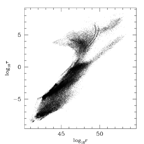
Figure 8: Left panel: Cumulative probability distribution of center-of-line optical depths of ART simulation cells within the virial extent. The three different lines correspond to the cell optical depth distribution in Ly-$\alpha$ (solid), Ly-$\delta$ (dotted) and Ly-limit (dashed) photons. Right panel: Ly-$\alpha$ center-of-line optical depth of the simulation cells within the virial extent of the emitter plotted against the cell recombination rate. Since only cells with the highest recombination rates ($\geq 10^{51}$ s^-1 or, equivalently, luminosities roughly $\geq 5\times 10^{50}$ photons s^-1) need to be used as source cells, and almost all of these cells have $\tau\geq 10^{3}$, roughly speaking our ’on-the-spot’ approximation is satisfactory (see text for details).

One assumption that we make is that the cascading of the Lyman series photons, as well as the re-emission and re-absorption of photons from recombination to the ground state, is done ’on-the-spot’, namely, locally. In our case ”locally” means within the same simulation cell. This assumption is essential if one wants the Ly-$\alpha$ emissivity of a cell to depend on its own recombination rate only. If not, one faces the complicated situation where the Ly-$\alpha$ emissivity of one cell depends on the recombination rates and photon cascade processes that are happening in other cells as well. The validity of our assumption depends on the optical depth of Lyman series and ionizing photons when traversing a typical cell in the simulation (and should also be affected somewhat by resolution). In the left panel of Figure 8 we show the optical depth probability distribution function for Ly-$\alpha$, Ly-$\delta$ and Ly-limit radiation. The distribution function has as independent variable the optical depth of simulation cells within 10 physical kpc ($\simeq$ virial extent) from the center of the emitter. These distributions are very similar, differing only by the values of $\tau$ because of different oscillator strengths and characteristic frequencies. Clearly, in all cases more than half potential source cells are not optically thick, and this is expected to get worse for ionizing radiation beyond the Lyman limit. However, as shown in the right panel of Figure 8 the optical depth of a cell correlates with its recombination rate. In this figure the optical depth plotted is that for Ly-$\alpha$ photons, but it is easy to see how this scales approximately with optical thickness for other Lyman-series photons. Since only cells with recombination rates higher than $10^{51}$ s^-1 (or equivalently with luminosities higher than roughly $5\times 10^{50}$ photons s^-1) are used as source cells, our ’on-the-spot’ assumption seems pretty satisfactory, if not always accurate. It becomes less and less accurate the higher we go in the Lyman series, and of course beyond the Lyman limit but for the time being we content ourselves with this approximation, given the complexities introduced when this assumption is not adopted. We will investigate this point further in the future.

Lastly, to get an idea about the physical conditions of the highest recombination rate (luminosity) source cells, they consist of two classes with respect to temperature and neutral hydrogen fraction: one class contains cold gas elements ($T\sim 10^{3}$K), with a neutral hydrogen fraction $>0.9$ (and high gas number density). The second class of very luminous cells consist of warmer gas elements ($T\sim 10^{4}$ K and a bit higher). In the context of Ly-$\alpha$ cooling radiation, discussed in the next section, the first class of cells are unable to cool via atomic hydrogen cooling since they are cold, whereas the second class of most luminous cells could cool via atomic hydrogen cooling temperature-wise, but that is not happening because these cells are highly ionized.

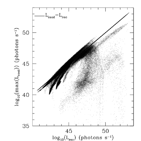
Figure 9: Maximum cooling Ly-$\alpha$ luminosity, $L_{cool}$, plotted against recombination Ly-$\alpha$ luminosity, $L_{rec}$, for all ART simulation cells within the virial extent of a Ly-$\alpha$ emitter at $z\simeq 8$. The cooling luminosity is the maximum possible Ly-$\alpha$ luminosity from cooling because it is derived assuming that all cooling radiation is emitted in Ly-$\alpha$ photons. The solid line shows the case where the two luminosities are equal. Since, as discussed in the text, only cells with luminosities roughly above $5\times 10^{50}$ photons s^-1 contribute significantly to the luminosity of the emitter, this figure shows that recombination is dominant over cooling Ly-$\alpha$ radiation.

3.2.2 Ly-$\alpha$ photons from collisional excitations

A collisional emission mechanism whose importance for the simulated objects can be assessed relatively easily is that of atomic hydrogen cooling. Using the expression by Hui & Gnedin (1997) for the hydrogen cooling rate (used in the ART simulations analyzed here), and assuming for the moment that this energy is all emitted in the form of Ly-$\alpha$ photons, we obtain for the luminosity (number of Ly-$\alpha$ photons/s) emitted by a cell

$$L_{cool}=4.6\times 10^{-8}\frac{e^{-1.18355/T_{5}}}{1+T_{5}^{0.5}}n_{e}n_{HI}V\,$$ (27)

with $T_{5}$ the temperature in units of $10^{5}$ K. This is compared with the recombination luminosity $L_{rec}$ ($\simeq 0.68r$) in Figure 9. Taking into account the results of the convergence test performed to specify what is the minimum cell luminosity that needs to be taken into account ($\sim 5\times 10^{50}$ s^-1), we see that the cells which are relevant are cells where recombination processes dominate, as can be seen in Figure 9. Namely, similar to previous studies (e.g., Fardal et al., 2001) we find that the cooling radiation Ly-$\alpha$ contribution is subdominant compared to the recombination contribution, hence in what follows we focus only on the latter.

3.2.3 Supernovae Remnants (SNR)

A Ly-$\alpha$ source that yields Ly-$\alpha$ photons both from recombinations and collisional excitations is supernova remnants (SNR). Shull & Silk (1979) have computed the time-averaged Ly-$\alpha$ luminosity of a population of Type II SNR using a radiative-shock code. They find that the Ly-$\alpha$ luminosity of a galaxy due to SNR is $L_{SNR}=3\times 10^{43}n_{H}^{-0.5}E_{0}^{0.75}\dot{N}_{SN}$ ergs/s, with $n_{H}$ the ambient density in cm^-3, $E_{0}$ the typical supernova energy in units of $10^{51}$, and $\dot{N}_{SN}$ the number of supernova per year. Strictly speaking, this quantity also depends on the assumptions on the IMF, and the lower and upper stellar masses of the mass range over which the IMF is to be integrated. This expression includes both contributions, from recombination and collisional emission mechanisms: from UV and X-ray ionization (coming from the hot SNR interior) of the surrounding medium and from cooling shells, respectively. A thorough investigation of the relative importance of SNR Ly-$\alpha$ emission with respect to that from young stars photoionization has been carried out by Charlot & Fall (1991, 1993). The general conclusion reached is that for a broad range of physical conditions and assumptions, the SNR contribution is at best a factor of 2.5 less than that from stellar ionizing radiation. These results make the effort to include the (anyway not resolved in ART simulations) SNR contributions superfluous.

3.3 The Ly-$\alpha$ emitter before RT

To get an idea of the size of the emitting region, the prevailing physical conditions, and for comparison with results obtained later after including RT, in this subsection we briefly present the emission spectrum and image of the emitter as they would appear to an observer at $z=0$ if the Ly-$\alpha$ photons escaped without any scattering. An image and a spectrum of the emitter along a certain direction of observation is shown in the left and right panel, respectively, of Figure 10.

The image is a surface brightness map (in units of ergs s^-1 cm^-2 arcsec^-2) of a roughly $1.4\times 1.4$ arcsecs² field which corresponds to approximately one third of the virial extent of the dark matter halo the emitter lives in (with the virial extent $\simeq 20$ physical kpc in diameter). There are two distinct emission regions, each one corresponding to the two progenitors that merged and formed this object. The color scale for the surface brightness is logarithmic. Clearly, the emission region is very small (the largest of the two structures is at most $\simeq 2-2.5$ physical kpc in diameter, if one includes the faintest pixels), compared for example to the virial extent of the dark halo. The resolution of this image is $0.01$ arcsecs ($\simeq$ 0.05 physical kpc), at least 10 times higher than the best resolution currently available. As discussed before, for these results only cells with recombination rates higher or equal to $10^{51}$ s^-1 are used. The initial frequency is chosen according to a Voigt profile that is sampled for each cell out to $10$ Doppler widths and shifted around the bulk (peculiar + Hubble) velocity component along the direction of observation. The number of photons used ($3\times 10^{5}$) has been determined after a convergence study. Note that when we study the convergence with respect to the number of photons we take into account that this must be done in parallel with how far away in the wings we go when sampling the emission Voigt profile of each cell, since the higher the number of photons used the better one can sample frequencies further away from resonance. The convergence procedure gave the aforementioned number of photons and initial emission frequency range (i.e., 10 thermal Doppler widths).

In the right panel of Figure 10, the frequency resolution is $\lambda/\Delta\lambda\sim 50000$. The line shape has converged, namely the peaks shown correspond to real velocity substructure. For example, the most pronounced peak at $\lambda=10952\AA$ corresponds to the component of the peculiar velocity along the direction of observation of the most luminous pixel of the image shown at the left panel (with coordinates on the image (0.24,-0.42) arcsecs, roughly). The dominant contribution to this pixel comes from the highest recombination cell of the emitter with a recombination rate equal to $\simeq 1.3\times 10^{55}$ s^-1 and a peculiar velocity component along the direction of observation equal to $0.27\times 10^{-3}$ the speed of light. As mentioned, for each emission cell the Voigt profile was used and sampled up to 10 thermal Doppler widths. The total width of the line however is dominated by the bulk velocity structure of the emitter. The full width of the line at the minimum flux level shown in the figure ($10^{-22}$ ergs $s^{-1}$ cm^-2 $\AA^{-1}$) is roughly $15\AA$ (with the width if bulk velocities are set to zero being less than half this). This width corresponds to projected velocities along the direction of observation roughly in the $[-200,200]$ km/s range (this is just approximate, note however that the line is not symmetric around the rest frame resonance). This velocity range is what is expected given the peculiar velocities of the emitting cells. Also shown is the spectrum of the smallest of the two substructures (dotted line) of the image shown in the left panel. One can easily infer what the spectrum of the large Ly-$\alpha$ substructure looks like.

The results discussed in this section may be specific to the emitter at hand, but the considerations themselves are pretty general. The same kind of procedure must be repeated for each individual emitter identified in the simulations.

     

Figure 10: Left panel: Image of Ly-$\alpha$ direct emission (i.e., assuming the Ly-$\alpha$ photons escape directly to the observer after they are produced). The approximately $1.4\times 1.4$ arcsecs² ($\simeq 6.5\times 6.5$ physical kpc) field corresponds to roughly one third of the virial extent of the dark matter halo where the emitter lives. The surface brightness (SB) is bolometric and in units of $\rm{ergs}\ \rm{s}^{-1}\rm{cm}^{-2}\rm{arcsecs}^{-2}$. The SB color scale is logarithmic. The object had undergone a recent merger, that is why there are two distinct luminous blobs that dominate the emission. Right panel: Initial Ly-$\alpha$ injection spectrum. Shown are the total spectrum (solid line), namely the spectrum for the image shown in the left panel, and the spectrum of the smallest of the two blobs in the image (dotted line). Note that the wavelength is in $10^{4}\AA$ (i.e., $\mu m$). The dashed line shows the Ly-$\alpha$ resonance for $z\simeq 8$. See text for discussion of the structure of the line.

3.4 The Ly-$\alpha$ emitter after RT

It is interesting to first treat the emitter as a finite configuration. In this case, as soon as the photons exit this configuration (whose size is taken to be roughly equal to the virial extent of the object, namely 10 physical kpc) they travel towards the observer. In other words at first we ignore the effect of the GP absorption. This context is pretty similar to that of §2.2 and §2.2.3. We focus on the emergent spectrum shown with the solid line in the left panel of Figure 11 .

     

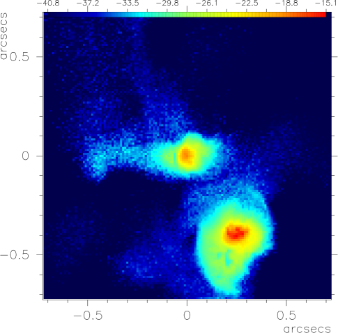
Figure 11: Left panel: Emerging Ly-$\alpha$ emission spectrum before adding the Ly-$\alpha$ Gunn-Peterson absorption (GPA) (no GPA, solid line), with the GPA but without the red damping wing (GP, no DW, short-dashed line), and with GPA and the damping wing (GPA+DW, dotted line). Note that the wavelength is in $10^{4}\AA$ (i.e., $\mu m$). The long-dashed line shows the Ly-$\alpha$ resonance for $z\simeq 8$. Right panel: Image of the Ly-$\alpha$ emitter after RT, GPA and DW. The $1.4\times 1.4$ arcsecs² ($\simeq 6.5\times 6.5$ physical kpc) field corresponds to roughly one third of the virial extent of the dark matter halo where the emitter lives. The surface brightness (SB) is bolometric and in units of $\rm{ergs}\ \rm{s}^{-1}\rm{cm}^{-2}\rm{arcsecs}^{-2}$. The SB color scale is logarithmic.

The spectrum converges if $3\times 10^{5}$ photons are used, namely if the same number of photons are used as the number of photons needed for the initial emission results (discussed in §3.3) to converge. Of course, the higher the number of photons the better one samples low intensity wavelengths. We find that the number of photons used affects wavelength ranges with flux less than about $10^{-22}$ ergs s^-1 cm^-2 $\AA^{-1}$. The spectrum shown in Figure 11 is produced using $10^{7}$ photons. The spectral resolution used in the figure is $\lambda/\Delta\lambda\simeq 5000$, whereas the spectrum is identical if ten times better resolution is used. We have performed a large set of convergence tests among which the most interesting are for different (smaller) cores for the acceleration scheme discussed in §2.3.2, and /or a larger minimum $\tau_{0}\phi(x_{i})$ for which the acceleration scheme discussed in §2.3.1 is used. Our results are pretty robust, as should following the discussion in §2.3.1 and 2.3.2 with respect to the one cell convergence results.

Even though meant for a slab, it is interesting to check if some predictions of the Neufeld solution, such as the frequency where the spectrum has a maximum ($\simeq 0.9(\alpha\tau_{0})^{1/3}$), are roughly in agreement with the spectrum of the simulated emitter. Of course, the Ly-$\alpha$ emitter environment is neither isothermal nor homogeneous, and it is not obvious how to define an ’effective’ temperature and optical depth for these purposes. Thus, focusing on order of magnitude checks, setting the expression for the frequency where the peak emission occurs in a slab equal to the frequency where the spectrum of the emitter peaks (say in red wavelengths) one finds that the ’effective’ optical depth and ’effective’ temperature of the equivalent slab (i.e., the slab that would give a spectrum with peak at the frequencies where the emitter spectrum peaks) roughly satisfy the relation $\tau_{0}T\simeq 1.4\times 10^{10}$ with $T$ measured in eV. The effective optical depth will be at least equal to the most optically thick cell the photon found itself in. Since the emission originates from the most optically thick cells (see Figure 8), $\tau_{0}$ will be at least $10^{3}$. If we assume for example a temperature $T=10^{5}$K, the above relation yields $\tau_{0}\simeq 10^{9}$ which is roughly the optical depth from the center of the object to its virial radius along the direction of observation. Thus, the maximum of the spectrum is roughly where it is expected to be if one assumes the scaling from the Neufeld solution ($\simeq 2550$ km/s).

The emerging spectrum looks pretty similar to the spectrum that would emerge from a static configuration, namely it has two quite similar peaks, one to the red and one to the blue of the Ly-$\alpha$ resonance. Note however that the peaks are not really symmetric, since the flux decreases more rapidly near the resonance. The width of the blue peak at a flux level of $10^{-22}$ ergs s^-1 cm^-2 $\AA^{-1}$ is roughly 180 $\AA$ or $\simeq 5000$ km/s. We obtain quite a similar spectrum if we set the bulk velocity field to zero in the code, that is kinematics do not seem to play a crucial role in this case. In the case of the specific Ly-$\alpha$ emitter and for the specific direction of observation, analyzing the bulk velocity field (i.e., the peculiar velocity field since the Hubble expansion is negligible at the distances we are working) we find that there is some net infalling motion, but with significant transverse velocity components as well. Hence, the obtained static–like spectrum does not come as a surprise. Furthermore, the peak asymmetry due to the existence of bulk fields depends on the relative magnitudes of the bulk and thermal velocities (e.g., if the bulk velocity is close to the thermal we do not expect a significant asymmetry since one scattering can give, e.g., a red photon moving in a contracting medium a large enough shift to erase the effect of the contraction) which varies from cell to cell, and it also depends on the optical thickness. Since thermal velocities are typically small compared to bulk velocities in simulations, the optical thickness is a more crucial factor. For such extremely optically thick media where the spectrum is expected to have in the context of the Neufeld solution a typical frequency of $\simeq 2550$ km/s, bulk velocities of at most some hundreds km/s will not really favor blue versus red photons (even if the bulk motion was purely inwards) that much, since both red and blue photons see a very optically thick medium.

It would be interesting to have a sense of what is the number of scatterings each photon undergoes before exiting. With the acceleration methods that we have to use though it is difficult to keep track of this quantity. A simple way to obtain an order-of-magnitude idea of the number of scatterings in such or, at least, similar configurations can be obtained by one of the examples discussed in §2.2.3. For the most optically thick case ($\tau_{0}\simeq 8.3\times 10^{6}$) and a point source emitting photons that propagate in a stationary medium the number of scatterings in one run of $\simeq 2000$ photons varies from $2.5\times 10^{3}$ up to $4\times 10^{7}$, with an average of $8.3\times 10^{6}$, and a median of $6.6\times 10^{6}$. Two thirds of the photons are in the $[4.6\times 10^{6},2.1\times 10^{7}]$ scatterings range. More generally, we find that similar to the Neufeld problem, the average number of scatterings in this spherical configuration scales linearly with optical depth at such thick media (see discussion in §2.2.1), with the proportionality constant of order unity. From this linear scaling of the average number of scatterings with optical depth, one can obtain a rough idea of the average number of scatterings of photons in the simulation environments (for the cell optical depth range in the simulations see, e.g., the left panel of Figure 8). These numbers also make clear why it is absolutely not feasible to perform Ly-$\alpha$ RT in the much thicker and more complicated simulation environments without some acceleration schemes.

Photons at very optically thick regions have to shift off resonance significantly to escape, and hence are the ones responsible for the significant line width of the spectrum (along with the $1/x^{2}$ behavior of the wing optical depth, as discussed previously). It is meaningful to ask whether one should really care about these photons, or instead ignore them because may be they are trapped indefinitely (for any practical purpose) in the dense cells and do not participate in the radiation propagation. To answer this question we estimate the photon diffusion time and compare it to the sound crossing and dynamical time scales (other time scales, such as the Hubble time scale for example which is $\sim 1$ Gyr at $z=8$ are clearly large enough to be non-relevant). Same as with the number of scatterings, to find the exact diffusion times one should follow the detailed RT. Given our acceleration methods this is not done. Instead we use some useful scalings. Since the average number of scatterings in very optically thick media is roughly equal to $\tau_{0}$, then the diffusion time is roughly $t_{d}\simeq N_{sc}l_{mfp}/c$ with $l_{mfp}$ the mean free path between scatterings defined through $\langle\tau\rangle=\int_{0}^{\infty}\tau e^{-\tau}d\tau=1$. In other words, since $\tau_{0}=n\sigma(x=0)L$, $\tau=n\sigma(\tilde{x})l$, then the mean free path in units of the total (half) width of the slab is $\sigma(x=0)/\sigma(\tilde{x})1/\tau_{0}$, with $\sigma(x=0)$ the cross section at the line center and $\sigma(\tilde{x})$ the cross section calculated at an effective $\tilde{x}$ so that the above definition for the mean free path is valid. Substituting in the expression for $t_{d}$ we obtain $t_{d}\sim\sigma(x=0)/\sigma(\tilde{x})L/c$. For a slab with $\tau_{0}=10^{6}$ we obtain a mean number of scatterings equal to $9.5\times 10^{5}$ and a median equal to $7.2\times 10^{5}$, whereas $67\%$ of the photons have between $5.1\times 10^{5}$ and $2.3\times 10^{6}$ scatterings. For the mean free path we find a mean equal to $2.4\times 10^{-5}$, a median equal to $1.9\times 10^{-6}$ and $67\%$ of the scatterings correspond to mean free paths between $1.4\times 10^{-6}$ and $7.7\times 10^{-6}$, all in units of the (half) width of the slab $L$. For the total distance traveled by the photons before escaping, we find an average distance of 40.2, a median of 32.3 – implying a $\sigma(x=0)/\sigma(\tilde{x})$ ratio of order 10 – whereas $67\%$ of photons exit after traveling a distance between 16.7 and 96.3, with these numbers as before in units of the width of the slab. Based on spatial random walk arguments one would have $N_{sc}\sim\tau_{0}^{2}$, hence the distance before escape would be $\sim\tau_{0}$ or $10^{6}$ for the specific example we use here. However, as discussed in §2.2.1 $N_{sc}$ scales linearly with $\tau_{0}$ and this makes a big difference. We find that the sound crossing time is significantly higher than the dynamical time for most simulation cells, hence the latter is the relevant time against which the diffusion time must be compared. We find that the dynamical time scale is at least three orders of magnitude or more larger than $L/c$ which is within a factor of order $10^{2}$ – for the various physical conditions in the simulation cells – representative of $t_{d}$. Note that this comparison also justifies the use of ’static’ simulation outputs where the RT is performed, even though we plan on investigating the possibility of incorporating the RT scheme into the dynamical evolution in the simulations. Furthermore, the effect of the simulation resolution on these conclusions will be investigated in a future study.

The scattering process diffuses the initial number of emitted photons on a larger area and hence lowers the number surface brightness (i.e., number per s cm² arcsec² rather than energy per s cm² arcsec²). In general the surface brightness itself can go either up or down, depending for example on the velocity structure of the medium. To quantify this effect on a photon-by-photon basis we choose to calculate the distance on the plane of the image between the initial emission point and the point (pixel) where the photon makes its maximum contribution to the image (see §2.4 on how spectra and images are obtained). We find that these distances vary from roughly $10^{-3}$ to $10$ physical kpc, with a median of 0.27 kpc and a mean of 0.31 kpc. Given that the largest of the two emission regions has a diameter of $\sim 2-2.5$ physical kpc (see, Figure 10), this means that the ’size’ of the luminous part of the object increases on average by more that 10% due to scattering. If, instead, we focus on the region where a certain fraction of photons originates from we obtain quite similar results. For example, ignoring the effects of RT, $90\%$ of the emitted photons that would reach the observer would originate within a radius of roughly 2.5 physical kpc. The same percentage of photons after taking into account RT would come from a radius of roughly 2.9 physical kpc.

So far we have been ignoring the GP absorption. When adding this absorption we consider two distinct cases. In the first case we include the red damping wing of the GP absorption, and in the second case we set it equal to zero. The latter best-case scenario is what would happen if for example the emitter was inside the HII region of a very bright quasar. The spectrum obtained in the first case is shown with the dotted line in the left panel of Figure 11, whereas the spectrum in the second case is shown with the short dashed line. An image of the emitter as would appear on earth with the GP absorption and the damping wing included is shown in the right panel of Figure 11.

Not surprisingly, when the damping wing is not taken into account the spectrum is identical with that before the GP absorption with the difference that all flux blueward of the Ly-$\alpha$ resonance is missing. When including the damping wing the maximum flux is suppressed by roughly a factor of 61.7 with respect to the maximum flux without it. This line is still quite wide, with a width of approximately 1370 km/s at a flux level of $10^{-21}$ ergs s^-1 cm^-2 $\AA^{-1}$, and a FWHM roughly $620$ km/s.

Lastly, these results have converged with respect to both the number of photons and the radius where the detailed RT stops (and beyond which the GP absorption is added). More specifically, we find that the number of photons required for the initial (no RT) emission to converge ($3\times 10^{5}$) is enough for the with RT and GP absorption results. And, the results also converge if a 10 physical kpc radius is used for the detailed RT and beyond that the GP absorption is added. Convergence has been checked also with respect to the minimum cell initial luminosity considered. We find that the results converge if the minimum luminosity discussed in §3.2 in the context of initial emission convergence is used.

3.5 Some additional physics considerations

Here we discuss the importance of collisions while the photons are propagating, as well as the possible role of dust (currently not taken into account).

3.5.1 Collisions

While the photons are undergoing scattering, collisions should be considered in the following three contexts: (i) collisional redistribution within the $n=2$ state; if for example a collision makes the atom go from the $2P_{3/2}$ to the $2S_{1/2}$, then the Ly-$\alpha$ photon is destroyed through a 2 photon decay of the $2S_{1/2}$ state. If instead the collision takes it to the $2P_{1/2}$, the scattering phase function will be different and hence it is relevant in either case to see how probable the collisional redistribution is (ii) collisional de-excitation of the $n=2$, in which case the photon is lost (iii) collisional broadening of the line, which could cause non-coherence in the rest frame of the atom. The RT code can take all these processes into account, but here we develop some intuition as to their importance. In fact, since, as will be shown, these processes are in practice negligible, the corresponding calculations in the RT code were switched off when producing the results presented in this study.

Referring to cases (i) and (ii), the largest collisional cross sections are for momentum changing transitions ($\Delta L=\pm 1$; e.g., Osterbrock, 1989). As discussed already, both collisions with electrons and protons are relevant, but protons are more significant in case (i), whereas electrons are more significant in case (ii). We have already calculated the probability per scattering that the $2P\rightarrow 2S$ transition of case (i) happens (see equation (26)). The maximum value of this probability for the conditions of the simulation cells is roughly $10^{-10}$ (assuming $T_{4}=1,n_{p}=10^{2}$ cm^-3, with the latter being of the order of the maximum proton number density of cells in simulations. The temperature dependence is so weak that it does not really matter what temperature one assumes, for order of magnitude estimates). So, unless a photon undergoes $10^{10}$ scatterings, collisions of the type (i) should not matter. The cells that are relevant for this are optically thick cells where the photons scatter repeatedly. Since as we saw $N_{sc}\simeq\tau_{0}$ and none of the simulation cells has $\tau_{0}$ larger than a few times $10^{9}$, collisions should not have a significant impact. Note that for most cells the number of scatterings for which collisions may start to matter is orders of magnitude higher than $10^{10}$ (i.e., what is described above is the worst case scenario as far as the effect of collisions is concerned since it assumes the maximum proton number density, present in very few cells). If these collisions do not matter then collisions of type (ii), which have smaller cross sections, should not matter either.

In case (iii), if the atom suffers collisions with other particles while it is emitting, the phase of the emitted radiation can be altered suddenly. If the phase changes completely randomly at the collision times, then information about the emitting radiation is lost and coherence is destroyed. In this case, in the rest frame of the atom, the line profile is Lorentzian but the total width is the natural width plus the frequency of collisions the atom experiences on average. Since the importance of this effect as well is determined by a comparison of the radiative decay time and the time between collisions (i.e., equation 26), from the above discussion it becomes clear that it is also negligible.

3.5.2 Dust

Dust absorbs Ly-$\alpha$ photons. Thus, one would assume that dust in the presence of scattering that traps photons, could have a significant effect, and that this may be true even if it is present in small amounts, as is expected to be the case for the $z\simeq 8$ emitter we discuss (with a metallicity roughly equal to 0.1 the solar metallicity). Indeed, Charlot & Fall (1991) found that only a tiny fraction of Ly-$\alpha$ photons escape from a static, neutral ISM even if there is a tiny amount of dust present. To include the effect of dust absorption in simulations we will have to implement a recipe to estimate the amount of dust. Even though one can come up with an observationally motivated recipe (albeit with unknown applicability at redshifts as high as 8), we postpone such a treatment for a future study, since the main focus of the current study is the Ly-$\alpha$ RT scheme (which nevertheless includes the probability per scattering that the photon will be absorbed, but this probability is currently set to 0).

However, the Ly-$\alpha$ emitter results we present in this study should not be taken as unrealistic, since it is not obvious how these results will change if we include the effects of dust. More specifically, many starforming galaxies are observed to have significant Ly-$\alpha$ luminosities (e.g., Kunth et al., 1998; Pettini et al., 2000), and this is usually attributed to the presence of galactic winds in these systems that allow the Ly-$\alpha$ photons to escape after much fewer scatterings than in the static medium case. These data seem to support the idea that it is the kinematics of the gas rather than the dust content that is the dominant Ly-$\alpha$ escape regulator.

Furthermore, Neufeld (1991) found that under suitable conditions the effects of dust absorption may actually increase rather than diminish the observed Ly-$\alpha$ line strength relative to radiation that suffers little or no scattering. This would happen for example in a multiphase medium consisting of dusty clumps of neutral hydrogen embedded within a relatively ’transparent’ medium. If most of the dust lies in cold neutral clouds then Ly-$\alpha$ photons, not being able to penetrate those clumps, will not be affected as much by the presence of dust (see also Hansen & Oh, 2005). Although there is no direct observational evidence to support this structure for the ISM (i.e., that dust lies preferentially in cold, neutral hydrogen clumps, even though the clumpiness in the distribution of neutral hydrogen itself seems to be established observationally (see Hansen & Oh, 2005, and references therein)), such a morphology of the dust and atomic hydrogen distribution could help account for the lack of strong correlation between dust content – inferred from metallicity or submillimeter emission – and Ly-$\alpha$ equivalent width. For example, some dust-rich galaxies have substantially higher Ly-$\alpha$ escape fraction than less dusty emitters (Kunth et al., 1998, 2003). In addition, Giavalisco et al. (1996) found that there is no correlation between the Ly-$\alpha$ equivalent widths and the slope of the UV continuum, which is a measure of the continuum extinction and hence of dust content.

Another reason why it is not obvious how the results presented here will change if we take dust into account, is that in the current version of the ART code molecular hydrogen forms only through the catalytic action of electrons. When molecular hydrogen formation on grains is included in the code, some of what is currently taken to be neutral atomic hydrogen will transform into molecular hydrogen, hence this effect will decrease the optical thickness of what currently are the thickest cells.

4 Summary

We develop a Ly-$\alpha$ RT code applicable to gasdynamics cosmological simulations. High resolution, along with appropriately treated cooling can lead to very optically thick environments. Solving the Ly-$\alpha$ RT even for one very thick simulation cell takes a long time. Solving it for the whole simulation box, or a significant fraction of it, takes unrealistic time. Thus, we develop accelerating schemes to speed up the RT. We treat the moderately thick cells by skipping the numerous core scatterings which are not associated with any significant spatial diffusion, and go directly to the scattering that takes the photon outside of the core. We use depth dependent core definitions, and find that quite large core values can be used. For the very optically thick cells we motivate our treatment from the classical problem of resonant radiation transfer in a semi-infinite slab. We find that with some modifications, since the simulations have cubic cells rather than slabs, we can use the analytical solution derived by Neufeld (1990) for the problem of the semi-infinite slab. With these accelerating methods, along with the parallelization of the code we made the problem of Ly-$\alpha$ RT in the complex environments of cosmological simulations tractable and solvable. Even though our approach assumes a cell structure for the simulation outputs, as is inherently the case in AMR codes, the Ly-$\alpha$ RT code we discuss is applicable to outputs from all kinds of cosmological simulation codes. This is true since one can always create an effective mesh by interpolating the values of the various physical parameters.

We perform a series of tests of the RT code, and then we apply it to ART cosmological simulations. We focus on the brightest emitter in those simulations at $z\simeq 8$. A first interesting result for this emitter pertains to its intrinsic emission region and mechanisms. The emission region consists of two smaller regions, each corresponding to one of the two main progenitors that merged to form the emitter at $z\simeq 8$. Both regions are pretty small, with the larger of the two having a diameter of $2-2.5$ physical kpc. Furthermore, recombination produced Ly-$\alpha$ photons is the dominant intrinsic Ly-$\alpha$ emission mechanism, with collisional excitation and SNR produced Ly-$\alpha$ photons being subdominant. The intrinsic luminosity of the emitter is $4.8\times 10^{43}$ ergs/s, whereas the injection spectrum (i.e., initial emission spectrum) shows significant velocity structure.

After performing the Ly-$\alpha$ RT, but before adding the GP absorption, the emitter spectrum obtained resembles that of a very optically thick static configuration, despite the slight trend for inward radial motions. More specifically, we obtain the usual double horn spectrum. This happens because (i) even though there is some net inward radial motion, there are still significant tangential peculiar velocity components, and (ii) the optical depth is so high that velocities of order some hundreds km/s will not favor blue versus red photons (i.e., in order to escape, both kinds of photons have to shift off resonance much more than the shift because of peculiar velocities, thus none of the two kinds of photons is favored in particular because of the existence of bulk motions). Namely, the velocity information is in fact lost because of the extremely high optical depth. The width of the two horns is noticeably high ($\sim 5000$ km/s), but in agreement with what is expected for the high simulation column densities. The size of the emitter increases, since the scatterings disperse the photons on a larger area. We find that on the plane of the emitter image, a photon on average escapes at a distance of about $10\%$ of the initial (before RT) emitter size from the point it was originally emitted.

We include the GP absorption in two different ways: without and with the red damping wing. In the first case the spectrum is identical to that when the GP is not included, with the difference that now we get only the red peak (rather than both the red and blue peaks). This case would correspond to the situation where the Ly-$\alpha$ emitter lies within the HII region of a very bright quasar. In the second case, where the damping wing is taken into account, the red peak is also affected. Its maximum flux is suppressed compared to when no damping wing is used by roughly a factor of 61.7. The resulting line after including the wing is still quite broad with a velocity width of about $1350$ km/s at a flux level of $10^{-21}$ergs s^-1 cm^-2 $\AA^{-1}$, and a FWHM of about $620$ km/s. The line is quite displaced redward from the Ly-$\alpha$ resonance, and reach a maximum monochromatic flux of $10^{-20.2}$ ergs s^-1 cm^-2 $\AA^{-1}$.

Attempting a detailed comparison with existing observations, or discussing detection prospects for an object such as the simulated emitter is beyond the scope of this study. We have studied only one emitter, and this for only one direction of observation since our main goal was to use it as an application for the Ly-$\alpha$ RT code. Thus, we do not have a large enough and representative simulation sample yet. Furthermore, currently the highest redshift where a Ly-$\alpha$ line has been observed is $\sim 6.6$ (Kodaira et al., 2003) and it is not known how different the properties of higher redshift emitters are from that of lower redshift ones. The most recent report at $z=9$ is that of Willis & Courbin (2005). This study finds no detections. The sky area coverage is possibly a significant factor contributing to this no detection result. Instead, we content ourselves here with a simple order of magnitude comparison. The intrinsic Ly-$\alpha$ luminosity of our emitter is consistent with luminosities reported in literature. For example, the highest Ly-$\alpha$ luminosity of the $z=5.7$ sample of Hu et al. (2004) is roughly $6\times 10^{43}$ ergs/s. Higher luminosities than those have been inferred for Ly-$\alpha$ blobs, rather than emitters. For example, the most luminous blob in the sample of Matsuda et al. (2004) has a Ly-$\alpha$ luminosity of $1.1\times 10^{44}$ ergs/s. Most observed Ly-$\alpha$ emitters are unresolved and so is expected to be the simulated emitter. Reported sizes for the observed objects are in the $\sim$ few kpc range (e.g., Hu et al., 2002). Ly-$\alpha$ blobs on the other hand are quite more extended, with sizes $\sim 100$ kpc (Matsuda et al., 2004). The widths of the (lower z) observed lines are typically a few hundred km/s, whereas the FWHM of the simulated line is roughly $620$ km/s. As discussed already, the velocity width of the ART emitter could be affected by the very high H column densities which will drop as soon as molecular hydrogen formation on dust grains is taken into account. In terms of the detectability, if one adopts the present day limit of ground based detections of $\sim 10^{-18}$ ergs s^-1 cm^-2 $\AA^{-1}$, clearly our simulated emitter would be orders of magnitude fainter. If the emitter is embedded within the HII region of a bright quasar, in which case the red damping wing will be suppressed, the brightness is marginally below the sensitivity of current ground based instruments. Note, however, that the prospects of detection will be much better for JWST which is expected to be able to detect $\sim 400$ times fainter objects than currently studied with ground based infrared telescopes.

References

- Adams (1972) Adams, T. F. 1972, ApJ, 174, 439
- Ahn et al. (2001) Ahn, S., Lee, H., & Lee, H. M. 2001, ApJ, 554, 604
- Ahn et al. (2002) —. 2002, ApJ, 567, 922
- Auer (1968) Auer, L. H. 1968, ApJ, 153, 783
- Avery & House (1968) Avery, L. W. & House, L. L. 1968, ApJ, 152, 493
- Barton et al. (2004) Barton, E. J., Davé, R., Smith, J.-D. T., Papovich, C., Hernquist, L., & Springel, V. 2004, ApJ, 604, L1
- Bouwens et al. (2004) Bouwens, R. J., Thompson, R. I., Illingworth, G. D., Franx, M., van Dokkum, P., Fan, X., Dickinson, M. E., Eisenstein, D. J., & Rieke, M. J. 2004, ApJ, 616, L79
- Bower et al. (2004) Bower, R. G., Morris, S. L., Bacon, R., Wilman, R. J., Sullivan, M., Chapman, S., Davies, R. L., de Zeeuw, P. T., & Emsellem, E. 2004, MNRAS, 351, 63
- Cantalupo et al. (2005) Cantalupo, S., Porciani, C., Lilly, S. J., & Miniati, F. 2005, astro-ph/0504015
- Cashwell & Everett (1959) Cashwell, E. & Everett, C. 1959, Monte Carlo Method for Random Walk Problems (New York: Pergamon Press)
- Chandrasekhar (1960) Chandrasekhar, S. 1960, Radiative Transfer (New York: Dover Publications)
- Charlot & Fall (1991) Charlot, S. & Fall, S. M. 1991, ApJ, 378, 471
- Charlot & Fall (1993) —. 1993, ApJ, 415, 580
- Delliou et al. (2005a) Delliou, M. L., Lacey, C., Baugh, C. M., Guiderdoni, B., Bacon, R., Courtois, H., Sousbie, T., & Morris, S. L. 2005a, MNRAS, 357, L11
- Delliou et al. (2005b) Delliou, M. L., Lacey, C., Baugh, C. M., & Morris, S. L. 2005b, astro-ph/0508186
- Dickinson et al. (2004) Dickinson, M. et al. 2004, ApJ, 600, L99
- Dijkstra et al. (2005a) Dijkstra, M., Haiman, Z., & Spaans, M. 2005a, astro-ph/0510407
- Dijkstra et al. (2005b) —. 2005b, astro-ph/0510409
- Fardal et al. (2001) Fardal, M. A., Katz, N., Gardner, J. P., Hernquist, L., Weinberg, D. H., & Davé, R. 2001, ApJ, 562, 605
- Field (1959) Field, G. B. 1959, ApJ, 129, 551
- Furlanetto et al. (2003) Furlanetto, S. R., Schaye, J., Springel, V., & Hernquist, L. 2003, ApJ, 599, L1
- Furlanetto et al. (2005) —. 2005, ApJ, 622, 7
- Giavalisco et al. (1996) Giavalisco, M., Koratkar, A., & Calzetti, D. 1996, ApJ, 466, 831
- Gnedin & Abel (2001) Gnedin, N. Y. & Abel, T. 2001, New Astronomy, 6, 437
- Gnedin & Prada (2004) Gnedin, N. Y. & Prada, F. 2004, ApJ, 608, L77
- Gould & Weinberg (1996) Gould, A. & Weinberg, D. H. 1996, ApJ, 468, 462
- Haiman & Spaans (1999) Haiman, Z. & Spaans, M. 1999, ApJ, 518, 138
- Haiman et al. (2000) Haiman, Z., Spaans, M., & Quataert, E. 2000, ApJ, 537, L5
- Hamilton (1940) Hamilton, D. R. 1940, Physical Review, 58, 122
- Hansen & Oh (2005) Hansen, M. & Oh, S. P. 2005, astro-ph/0507586
- Harrington (1973) Harrington, J. P. 1973, MNRAS, 162, 43
- Hu et al. (2004) Hu, E. M., Cowie, L. L., Capak, P., McMahon, R. G., Hayashino, T., & Komiyama, Y. 2004, AJ, 127, 563
- Hu et al. (2002) Hu, E. M., Cowie, L. L., McMahon, R. G., Capak, P., Iwamuro, F., Kneib, J.-P., Maihara, T., & Motohara, K. 2002, ApJ, 568, L75
- Hui & Gnedin (1997) Hui, L. & Gnedin, N. Y. 1997, MNRAS, 292, 27
- Hui et al. (1997) Hui, L., Gnedin, N. Y., & Zhang, Y. 1997, ApJ, 486, 599
- Hummer (1962) Hummer, D. G. 1962, MNRAS, 125, 21
- Jefferies & White (1960) Jefferies, J. T. & White, O. R. 1960, ApJ, 132, 767
- Kodaira et al. (2003) Kodaira, K. et al. 2003, PASJ, 55, L17
- Kravtsov (2003) Kravtsov, A. V. 2003, ApJ, 590, L1
- Kravtsov & Gnedin (2005) Kravtsov, A. V. & Gnedin, O. Y. 2005, ApJ, 623, 650
- Kunth et al. (2003) Kunth, D., Leitherer, C., Mas-Hesse, J. M., Östlin, G., & Petrosian, A. 2003, ApJ, 597, 263
- Kunth et al. (1998) Kunth, D., Mas-Hesse, J. M., Terlevich, E., Terlevich, R., Lequeux, J., & Fall, S. M. 1998, A&A, 334, 11
- Loeb & Rybicki (1999) Loeb, A. & Rybicki, G. B. 1999, ApJ, 524, 527
- Maier (2002) Maier, C. 2002, Ph.D. Thesis, Naturwissenschaftlich-Mathematische Gesamtfakultat der Universitat Heidelberg, Germany
- Matsuda et al. (2004) Matsuda, Y. et al. 2004, AJ, 128, 569
- Neufeld (1990) Neufeld, D. A. 1990, ApJ, 350, 216
- Neufeld (1991) —. 1991, ApJ, 370, L85
- Osterbrock (1962) Osterbrock, D. E. 1962, ApJ, 135, 195
- Osterbrock (1989) —. 1989, Astrophysics of Gaseous Nebulae and Active Galactic Nuclei (Mill Valey, CA: Univ. Sci.)
- Partridge & Peebles (1967) Partridge, R. B. & Peebles, P. J. E. 1967, ApJ, 147, 868
- Pelló et al. (2004) Pelló, R., Schaerer, D., Richard, J., Le Borgne, J.-F., & Kneib, J.-P. 2004, A&A, 416, L35
- Pettini et al. (2000) Pettini, M., Steidel, C. C., Adelberger, K. L., Dickinson, M., & Giavalisco, M. 2000, ApJ, 528, 96
- Phillips & Meszaros (1986) Phillips, K. C. & Meszaros, P. 1986, ApJ, 310, 284
- Rhoads et al. (2003) Rhoads, J. E., Dey, A., Malhotra, S., Stern, D., Spinrad, H., Jannuzi, B. T., Dawson, S., Brown, M. J. I., & Landes, E. 2003, AJ, 125, 1006
- Santos (2004) Santos, M. R. 2004, MNRAS, 349, 1137
- Santos et al. (2003) Santos, M. R., Ellis, R. S., Kneib, J., Richard, J., & Kuijken, K. 2003, ApJ, 606, 683
- Shull & Silk (1979) Shull, J. M. & Silk, J. 1979, ApJ, 234, 427
- Spergel et al. (2003) Spergel, D. N. et al. 2003, ApJS, 148, 175
- Spitzer (1978) Spitzer, L. 1978, Physical Processes in the Interstellar Medium (New Yorl: Wiley)
- Stanway et al. (2004) Stanway, E. R., Bunker, A. J., McMahon, R. G., Ellis, R. S., Treu, T., & McCarthy, P. J. 2004, ApJ, 607, 704
- Steidel et al. (2000) Steidel, C. C., Adelberger, K. L., Shapley, A. E., Pettini, M., Dickinson, M., & Giavalisco, M. 2000, ApJ, 532, 170
- Taniguchi et al. (2005) Taniguchi, Y. et al. 2005, PASJ, 57, 165
- Tasitsiomi (2006) Tasitsiomi, A. 2006, astro-ph/0601562
- Unno (1952) Unno, W. 1952, PASJ, 4, 100
- Weatherley et al. (2004) Weatherley, S. J., Warren, S. J., & Babbedge, T. S. R. 2004, A&A, 428, L29
- Willis & Courbin (2005) Willis, J. P. & Courbin, F. 2005, MNRAS, 357, 1348
- Wouthuysen (1952) Wouthuysen, S. A. 1952, AJ, 57, 31
- Yusef-Zadeh et al. (1984) Yusef-Zadeh, F., Morris, M., & White, R. L. 1984, ApJ, 278, 186
- Zanstra (1949) Zanstra, H. 1949, Bull. Astron. Inst. Netherlands, 11, 1
- Zheng & Miralda-Escudé (2002) Zheng, Z. & Miralda-Escudé, J. 2002, ApJ, 578, 33