Simulations of axisymmetric magnetospheres of neutron stars

Abstract

In this paper we present the results of time-dependent simulations of dipolar axisymmetric magnetospheres of neutron stars carried out both within the framework of relativistic magnetohydrodynamics and within the framework of resistive force-free electrodynamics. The results of force-free simulations reveal the inability of our numerical method to accommodate the equatorial current sheets of pulsar magnetospheres and raise a question mark about the robustness of this approach. On the other hand, the MHD approach allows to make a significant progress. We start with a nonrotating magnetically dominated dipolar magnetospheres and follow its evolution as the stellar rotation is switched on. We find that the time-dependent solution gradually approaches the steady state that is very close to the stationary solution of the Pulsar Equation found by Contopoulos et al.(1999). This result suggests that other stationary solutions that have the y-point located well inside the light cylinder are unstable. The role of the particle inertia and pressure on the structure and dynamics of MHD magnetospheres is studied in details, as well as the potential implications of the dissipative processes in the equatorial current sheet. We argue that pulsars may have differentially rotating magnetospheres which develop noticeable structural oscillations and that this may help to explain the nature of the sub-pulse phenomena.

1 Introduction

Pulsar magnetospheres are complicated electrodynamic systems that involve the acceleration of charged particles by the rotationally induced electric field, the electron-positron pair production, and the bulk outflow of magnetospheric plasma through the light cylinder. The pair production presumably occurs on the scale which is significantly smaller compared to the magnetospheric scale (the last is determined by the light cylinder radius $\varpi_{lc}=c/\Omega$). This suggests that that the global structure of pulsar magnetospheres may not depend on the details of the pair production mechanism which may enter the problem only in the form of boundary conditions. The simplest assumption is that the plasma supply is sufficiently plentiful to allow the MHD description throughout the whole magnetosphere. Although this may be not so in the case of slowly rotating or weakly magnetized pulsars [Hibschman & Arons 2001], it still makes sense to regard the MHD solution as a zero approximation model and a good reference point.

Although pulsar magnetospheres are generically three dimensional it is still reasonable to start with a much simpler axisymmetric case as it involves most of the basic physical elements of the general case. Michel[Michel 1973] and Scharlemann & Wagoner [Scharlemann & Wagoner 1973] first analysed the structure of the stationary axisymmetric pulsar magnetosphere in the limit of force-free electrodynamics where both the pressure and inertia of magnetospheric plasma are assumed to be vanishingly small. They found that in this case the problem is reduced to the following second order PDE that is now called the Pulsar Equation,

$$(1-x^{2})\left(\frac{\partial^{2}\Psi}{\partial x^{2}}+\frac{1}{x}\frac{\partial\Psi}{\partial x}+\frac{\partial^{2}\Psi}{\partial y^{2}}\right)-\frac{2}{x}\frac{\partial\Psi}{\partial x}=-{\cal A}(\Psi)\frac{d\cal A}{d\Psi},$$ (1)

where $x=\varpi/\varpi_{lc}$ and $y=z/\varpi_{lc}$ are the cylindrical coordinates normalised to the radius of the light cylinder and $\Psi$ is the magnetic flux function. This equation also involves the poloidal current function, ${\cal A}(\Psi)$, that is unknown. If this function is somehow specified the pulsar equation become a linear elliptic equation. However, the question of what actually determines the electric current function is not that obvious and is still debated [Mestel 1999, Beskin 2005]. The physical meaning of these functions is quite simple: $\Psi=\Phi/2\pi$, where $\Phi(x,y)$ is the magnetic flux through the axisymmetric circular loop given by $x=$const, $y=$const; ${\cal A}=2I/c$ where $I(x,y)$ is the total electric current flowing through the same loop. It is also worth mentioning that if we set $A_{\phi}(x=0)=0$ then $\Psi=A_{\phi}$ and that in a steady-state ${\cal A}=H_{\phi}$, where $A_{\phi}$ and $H_{\phi}$ are the covariant azimuthal components of the vector-potential $\mn@boldsymbol{A}$ and the magnetic field $\mn@boldsymbol{H}$ in the non-normalised basis of cylindrical or spherical coordinates.

Another important feature of this equation is the mathematical singularity at the light cylinder. It was argued by Ingraham[Ingraham 1973] that the condition of smooth passage through this surface together with the appropriate boundary conditions determine the unique electric current function of the pulsar equation (This property makes the problem somewhat similar to the classical eigenvalue problem in the theory of differential equations.) Ingraham[Ingraham 1973] even proposed an iterative algorithm for finding this function. In the same year Michel[Michel 1973] did actually find an exact solution to the pulsar equation in the case of split-monopole magnetic field that passed through the singular surface both continuously and smoothly. Although Michel did not use Ingraham’s approach his result supported Ingraham’s idea and raised expectations for finding smooth continuous solutions in more complicated realistic cases, like for example the magnetosphere of a rotating dipole, as well. (The recent observations of magnetospheric eclipses in the binary pulsar J0737-3039 have confirmed that the dipolar model may indeed be quite accurate [Lyutikov & Thompson 2005].)

The electric current of Michel’s solution has the same sign within the magnetosphere with the exception of the equatorial current sheet that provides current closure. Further analysis by Ingraham[Ingraham 1973] and Michel[Michel 1974] suggested that if the force-free solution for an axisymmetric rotating dipole existed then far beyond the light cylinder it should still closely resemble the split-monopole one. However, in the near zone the structure of the dipole magnetosphere was expected to be qualitatively different. Indeed, close to the star the effects of its rotation are relatively small and so must be the difference between the solutions for the rotating and the non-rotating magnetospheres. As the result, the so-called “dead zone” should exist where the magnetic field lines remain closed and the magnetospheric plasma co-rotates with the star.

However, the problem of finding the self-consistent global solution for dipolar magnetospheres turned out to be rather involved, even for the axisymmetric case of aligned rotator. For a very long time, the only attempts to construct such solutions involved utilisation of prescribed electric current functions. Such solutions would either exhibit kinks at the light cylinder or violate the conditions of force-free approximation at some relatively short distance from it, e.g. [Michel 1982, Beskin et al. 1993]. The break through came only recently then Contopoulos et al. (1999, hereafter CKF) have finally managed to solve the problem numerically. In this solution the dead zone continues all the way to the light cylinder where the so-called “Y-point” appears in the magnetic field structure whereas beyond the light cylinder it has the same topology as the split-monopole solution including an infinitely thin equatorial current sheet. The return current of the equatorial current sheet splits at the Y-point into two currents sheets that flow along the surface separating the dead zone from the open field zone. An additional finite width layer of return current exists just outside of the dead zone and around the equatorial plane.

Uzdensky [Uzdensky 2003] carried out asymptotic analysis of the force-free solutions in vicinity of the Y-point. It has turned out that in the presents of separating current sheets, similar to those found in [Contopoulos et al. 1999], the electromagnetic field becomes infinitely strong at the Y-point. He argued that this is unphysical and questioned correctness of the CKF-solution. As an alternative Uzdensky [Uzdensky 2003] considered the case with no current sheets, that is the case where the electric current returns within the equatorial layer of the open field zone only. In this case the electromagnetic field does not diverge at the Y-point but just outside of this point the electric field becomes stronger than the magnetic field signaling a breakdown of the force-free approximation. No such complications were found for the Y-point located inside the light cylinder. In fact, in this case the separating surface crosses the equator at the right angle so that the Y-point turns into a ”T-point”.

Gruzinov[Gruzinov 2005] also analysed the force-free solution in the vicinity of the Y-point located at the light cylinder in the presence of the current sheets and confirmed that in this case the electromagnetic field diverges at the Y-point. His analytical solution exhibits the angle of $77^{o}.3$ between the equatorial plane and the separating surface at the Y-point. In order to verify this he repeated the CKF-calculations with much higher spatial resolution and the results seemed to confirm the development of a singularity with the expected inclination angle of separatrices.

The next potentially very important step was made by Goodwin et al.[Goodwin et al. 2004] who realised that the dead zone does not have to extend all the way to the light cylinder but can be much smaller. Such solutions select their own electric current functions, smaller dead zones corresponding to weaker currents. In fact, the first solutions of the pulsar equation which described both the equatorial current sheet and the dead zones that were located deep inside the light cylinder were found by Lyubarskii[Lyubarskii 1990]. However, these solutions utilized a prescribed electric current function and, as the result, exhibited the breakdown of the force-free approximation – at a certain distance from the light cylinder the electric field became stronger than the magnetic field. Goodwin et al.[Goodwin et al. 2004] also included finite gas pressure inside the dead zone and showed that this allows solutions that remain nonsingular at the Y-point even when this point is located on the light cylinder. In this case their solution gives the inclination angle of the Y-point of $56^{o}.5$. However, the inertia associated with the gas pressure has not been taken into account and thus the self-consistency of such approach is questionable.

This idea of Goodwin et al.[Goodwin et al. 2004] was further explored by Timokhin[Timokhin 2005] who has constructed numerical solutions for force-free magnetospheres with the Y-point located within the light cylinder (with no finite gas pressure in the dead zone). He also pointed out that the pulsar spin-down rate depended not only on the size the light cylinder but also on the size of the dead zone and if the ratio of these scales were to evolve with the pulsar age then this could explain why the observed braking index of pulsars is smaller than the one derived from the models with the dead zone extending all the way up to the light cylinder.

Another interesting twist has been added by Contopoulos[Contopoulos 2005], who argued that during the pulsar evolution the potential gap separating the star surface from the polar cap magnetosphere grows in magnitude leading to a slower rotation of the open field lines compared to the star and the dead zone. In such a case, there is no a single light cylinder for the whole magnetosphere. Instead, the dead zone has its own light cylinder that is located inside the light cylinder of the polar cap. To illustrate this point Contopoulos(2005) constructed a set of numerical models of pulsar magnetospheres of this kind. The evolution of the angular velocity of the polar cap magnetosphere with pulsar age may also result in the lower values of the pulsar’s braking index.

In spite of this remarkable progress the method of pulsar equation has its obvious limitations. It does not address the question of stability of the steady-state solutions and it does not allow to study possible non-stationary phenomena in pulsar magnetospheres. Moreover, the numerical techniques that have been used to solve the pulsar equation may turn up to be rather difficult to adapt to the fully 3-dimensional problem of the oblique rotator. The obvious way of approaching these problem is to relax the stationarity condition and to solve the original system of time-dependent equations. Although the force-free electrodynamics was used to model various astrophysical systems since 1970s the focus was entirely on the steady-state equations. Only recently, the time-dependent equations have been subjected to a systematic study [Uchida 1997, Gruzinov 1999, Komissarov 2002a, Punsly 2001]. As the result it has been found that they form a simple hyperbolic system of conservations laws in many respects similar to relativistic MHD but only with the fast and the Alfvén hyperbolic waves [Komissarov 2002a]. Thus, a variety of standard numerical methods can be used to deal with these equations. The very first numerical simulations of this kind, of the monopole magnetospheres of black holes, seemed to confirm the suitability of this approach [Komissarov 2001]. However, further applications to somewhat more complex magnetic configurations revealed its limitations as the force-free approximation would often break down following development of strong current sheets [Komissarov 2002a, Komissarov 2002b, Spitkovsky 2004, Asano et al. 1999]. These results suggested to look for a more general mathematical framework that would allow to handle current sheets via introducing new channels of back reaction of plasma on the electromagnetic field. One of the most suitable options is the framework of resistive relativistic MHD. However, this approach remains rather poorly studied even now. Ideal relativistic MHD is a somewhat easier option and thanks to the recent effort by several groups, a significant expertise has been obtained in developing numerical methods for this system. This approach allows to take into account both the thermodynamic pressure of plasma heated in the current sheets but the dissipation of electromagnetic energy is entirely due to numerical resistivity that is not fully satisfactory.

Another alternative is resistive force-free electrodynamics with physical or artificial resistivity. If the current sheets of pulsar magnetospheres are indeed dissipationless then this approach might work provided that the utilized Ohm law allows evolution towards a dissipationless force-free state. The recent time-dependent simulations by A.Spitkovsky show that this approach may indeed be quite productive (the results were presented last summer at the conference on “Physics of Astrophysical Outflows and Accretion Disks”, KITP, Santa-Barbara, 2005.)

In this paper we report the results of new time-dependent axisymmetric simulations of rotating dipole magnetospheres of neutron stars within the frameworks of resistive force-free electrodynamics and ideal relativistic MHD. We only consider the case where the whole magnetosphere rotates with the same angular velocity and thus our results are not relevant to the model of Contopoulos[Contopoulos 2005]. This model will be a subject of a separate study. Note, that throughout the paper the graphic data are shown in the dimensionless units where the magnetic dipole moment $\mu=1$, the angular velocity of the star $\Omega$, and the speed of light $c=1$. Hence the cylindrical radius of the light cylinder $\varpi_{lc}=1$.

2 Common features of the simulations

Using the standard notation of the 3+1 approach the metric form of a general space-time can be written as

$$ds^{2}=(\beta^{2}-\alpha^{2})dt^{2}+2\beta_{i}dx^{i}dt+\gamma_{ij}dx^{i}dx^{j},$$ (2)

where $\gamma_{ij}$ is the metric tensor of “the absolute space”, $\alpha$ is the lapse function, and $\mn@boldsymbol{\beta}$ is the shift vector. For most purposes in physics of pulsar magnetospheres the flat space approximation suffices and one can enjoy the benefits of a global inertial frame where $\alpha=c$ and $\beta_{i}=0$ (see however Beskin 1990 and Muslimov & Tsygan 1990). This is exactly what was adopted in the numerical models of pulsar magnetospheres described in the Introduction and in this study as well. However, the computer codes used in the simulations are designed to work with a rather general axisymmetric and stationary space-times. Moreover, in the case of oblique rotator the frame rotating with the star seem to be more suitable as the solution may become stationary in this frame. In such a case $\mn@boldsymbol{\beta}$ is no longer vanishing and in the basis of spherical spacial coordinates

$$\beta_{r}=\beta_{\theta}=0,\ \beta_{\phi}=c\Omega\sin^{2}\!\theta r^{2},$$

and hence

$$\alpha^{2}=c^{2},\quad\mbox{and}\quad\beta^{2}=c^{2}\Omega^{2}\sin^{2}\!\theta r^{2},\$$

where $\Omega$ is the angular velocity of the frame.

In our simulations, the computational grid covers the axisymmetric domain $(r,\theta)=[r_{in},r_{out}]\times[0,\pi]$ so no symmetry condition is enforced at the equatorial plane. The cell size in the $r$-direction is such that the corresponding physical lengths in both directions are equal, $\Delta r=r\Delta\theta$. The “radiative” outer boundary, $r=r_{out}$, is always located so far away from the star that the light signal does not cross the computational domain by the end of the simulations – this ensures that waves produced near the star do not get reflected of the outer boundary at any rate.

As the Courant stability condition requires $\Delta t<\Delta r/c$, the suitable time step for the outer part of the computational domain is much larger than the one for its inner part. This allows us to reduce the computational cost of simulations via splitting the computational domain into a set of rings such that the outer radius of each ring is twice its inner radius and advance the solution for each $k$th ring with it its own time step, $\Delta t_{k}$, such that $\Delta t_{k+1}=2\Delta t_{k}$. Thus, one integration step of ring $k$ corresponds to two integration steps of ring $k-1$, four integration steps of ring $k-2$ and so on. As the result, the outer regions of the computational domain are progressively less expensive in terms of CPU time. This approach has already been successfully applied in recent MHD simulations of Pulsar Wind Nebulae [Komissarov & Lyubarsky 2004b].

The initial solution describes a nonrotating magnetosphere with exactly dipolar magnetic field,

$$B^{\hat{\phi}} = 0;$$

$$B^{\hat{r}} = 2\mu\cos\theta/r^{3};$$ (3)

$$B^{\hat{\theta}} = \mu\sin\theta/r^{3},$$

where $\mu$ is the magnetic dipole moment. At time $t=0$ the stellar rotation is suddenly switched on via an appropriate inner boundary condition. The simulations are then proceeded till it becomes clear whether the time-dependent solution relaxes to a steady state on scales comparable with the light cylinder radius or not. Steady-state solutions that are found in such a way are automatically stable to axisymmetric perturbations with wave-lengths exceeding the cell size.

3 Electrodynamic model

3.1 Equations

Following Komissarov[Komissarov 2004a] we write vacuum Maxwell’s equations as

$$\partial_{i}(\sqrt{\gamma}B^{i})=0,$$ (4)

$$(1/c)\partial_{t}B^{i}+e^{ijk}\partial_{j}E_{k}=0,$$ (5)

$$\partial_{i}(\sqrt{\gamma}D^{i})=4\pi\sqrt{\gamma}\kappa,$$ (6)

$$-(1/c)\partial_{t}D^{i}+e^{ijk}\partial_{j}H_{k}=(4\pi/c)J^{i}.$$ (7)

Here $\gamma=\det(\gamma_{ij})$ is the determinant of the metric tensor of the absolute space, $e_{ijk}=\sqrt{\gamma}\epsilon_{ijk}$ is the Levi-Civita tensor of the absolute space ($\epsilon_{123}=1$ for right-handed systems and $\epsilon_{123}=-1$ for left-handed ones.) The electric field, $\mn@boldsymbol{E}$, and the magnetic field, $\mn@boldsymbol{B}$, are defined via

$$E_{i}=\frac{\alpha}{2}e_{ijk}\,^{*}\!F^{jk},$$ (8)

and

$$B^{i}=\alpha\,^{*}\!F^{it},$$ (9)

where $\,{}^{*}\!F^{\mu\nu}$ is the Faraday tensor of the electromagnetic field, which is simply dual to the Maxwell tensor $F^{\mu\nu}$:

$$\,{}^{*}\!F^{\alpha\beta}=\frac{1}{2}e^{\alpha\beta\mu\nu}F_{\mu\nu}$$ (10)

where

$$e_{\alpha\beta\mu\nu}=\sqrt{-g}\,\epsilon_{\alpha\beta\mu\nu},$$ (11)

is the Levi-Civita alternating tensor of spacetime.

Figure 1: Representative force-free solution. The contours show the magnetic flux surfaces and the colour image shows $H_{\phi}$. Notice that the magnetic field lines are closed even beyond the light cylinder, $\varpi_{ls}=1$.

The differential equations (4-7) are supplemented with the following constitutive equations [Komissarov 2004a]:

$$cE_{k}=\alpha D_{k}+e_{kij}\beta^{i}B^{j},$$ (12)

$$cH_{k}=\alpha B_{k}-e_{kij}\beta^{i}D^{j}.$$ (13)

$$J^{k}=(\alpha/c)j^{k}-\kappa\beta^{k}.$$ (14)

Note, that 1) the components of all vectors and tensors appearing in these equations are measured in the non-normalised coordinate basis, $\{\partial_{i}\}$, of spacial coordinates; 2) $\mn@boldsymbol{D}$, $\mn@boldsymbol{B}$, $\mn@boldsymbol{j}$, and $\kappa$ are the electric field, the magnetic field, the electric current density, and the electric charge density as measured by a local observer at rest in the absolute space. The 4-velocity of this observer is

$$n^{\nu}=\frac{1}{\alpha}(c,\beta^{i});$$

In the inertial frames of flat spacetime $\mn@boldsymbol{E}=\mn@boldsymbol{D}$ and $\mn@boldsymbol{B}=\mn@boldsymbol{H}$.

The final equation that is needed to close the system is the Ohm law. In strongly magnetized plasma the conductivity is no longer isotropic and under rather general conditions

$$\mn@boldsymbol{j}=\sigma_{\parallel}\mn@boldsymbol{D}_{\parallel}+\sigma_{\perp}\mn@boldsymbol{D}_{\perp}+\mn@boldsymbol{j}_{d},$$ (15)

where

$$\mn@boldsymbol{j}_{d}=\kappa c\frac{\mn@boldsymbol{D}\!\times\!\mn@boldsymbol{B}}{B^{2}}$$ (16)

is the drift current. Unless the magnetosphere has scarce supply of electrically charged particles ,“charge starved”, the parallel conductivity is very larger that leads to small residual parallel component of electric field,

$$\sigma_{\parallel}\rightarrow\infty,\quad\mbox{ }\quad\mn@boldsymbol{D}_{\parallel}\rightarrow 0.$$ (17)

However, the strong magnetic field of pulsar magnetospheres effectively suppresses conductivity across the magnetic field lines (unless the electric field is even stronger than the magnetic one; this may be the case inside some current sheets.) So we can put

$$\sigma_{\perp}=0\quad\mbox{if}\quad B^{2}>D^{2}.$$ (18)

As shown in [Komissarov 2004a], in this limit we approach the approximation of force-free electrodynamics.

Within current sheets this simple prescription is unlikely to hold. On one hand, in the area of high current density one may expect strong anomalous resistivity leading to significantly reduced $\sigma_{\parallel}$. As the result, the current sheet may become unstable to the tearing mode of reconnection [Lyutikov 2003]. Since our intention at this point is merely to see if we can construct idealized numerical solutions that are more-or-less force-free and thus can be compared with the steady state solutions of the Pulsar Equation we will ignore this physical effect for the time being. On the other hand, the mere symmetry of the aligned rotator magnetosphere suggests that sooner or later the magnetic field of force-free solution will become very small in the equatorial plane beyond the light cylinder, thus leading to unavoidable breakdown of the $D^{2}<B^{2}$ condition of the force-free approximation. In such a case of relatively weak magnetic field the conductivity is expected to become much less anisotropic and we will assume that

$$\sigma_{\perp}=\sigma_{\parallel}\gg 1\quad\mbox{if}\quad B^{2}<D^{2}.$$ (19)

Notice, that the expression (16) for the drift current should also be modified in this case as it implies that the drift speed

$$\mn@boldsymbol{v}_{d}=c\frac{\mn@boldsymbol{D}\!\times\!\mn@boldsymbol{B}}{B^{2}}$$ (20)

becomes higher then the speed of light. We have tried several modifications for the $v_{d}$ including

$$v_{d}=c\frac{\mn@boldsymbol{D}\!\times\!\mn@boldsymbol{B}}{\max(B^{2},D^{2})}$$ (21)

which is likely to underestimate $v_{d}$ in the current sheet and

$$v_{d}=c\frac{\mn@boldsymbol{D}\!\times\!\mn@boldsymbol{B}}{|\mn@boldsymbol{D}\!\times\!\mn@boldsymbol{B}|}\quad\mbox{if}\quad B^{2}<D^{2}$$ (22)

which certainly overestimates it. The actual value of conductivity in the current current sheet remain a free parameter.

To find numerical solutions of Maxwell’s equation, in particular the solutions that are presented in the next section, we used the Godunov-type numerical scheme described in Komissarov[Komissarov 2004a].

3.2 Numerical simulations

The most striking and at first somewhat perplexing result of our electrodynamic simulations of pulsar magnetospheres is demonstrated in figure 1 – contrary to what is found in the steady-state solutions of the pulsar equation the magnetic field lines remain close even outside of the light cylinder. Moreover, the solution seems to be rather insensitive to the details of the model for $\sigma_{\perp}$ and remains qualitatively the same even in the case $\sigma_{\perp}=0$ (In fact, the solutions exhibited convergence in the limit $\sigma_{\perp}\to 0$.)

The question of whether the field lines extending beyond the light cylinder should open up or not is in fact rather involved. One of the arguments often put forward in its discussion concerns the requirement for the speed of charged particles that fill the magnetosphere to remain smaller than the speed of light. In the drift approximation the charged particles move along the rotating magnetic field lines like beads on wire – their motion is a composition of the rotational motion of the field line (the “wire”) and the sliding motion of the particle (the “bead”) along the field line. Within the light cylinder the speed of the rotational motion is less than the speed of light and the bead does not have to slide along the wire, but this is no longer the case beyond the light cylinder. Here the total speed of the bead can remain less than $c$ only if it also slides along the wire and only if the wire is twisted in the azimuthal direction (In such a case the sliding motion may help to reduce the azimuthal component of the bead velocity.) These conditions may well be satisfied everywhere along the open field lines but not along the closed ones. Indeed, such field lines cannot have an azimuthal component in the equatorial plane because of the symmetries of the problem. Thus, one may expect spinning up of the charged particles till their inertia becomes important and the centrifugal force opens up the closed field lines.

On the other hand, the drift approximation itself may breakdown and the charges may start moving across the magnetic field well before their inertia becomes dynamical significant. One can look at this breakdown of the drift approximation from another prospective. Beyond the light cylinder the electric field of a force-free solution becomes stronger than the poloidal component of the magnetic field and thus stronger than the total magnetic field in regions where the azimuthal component of magnetic field vanishes. Such a strong electric field is capable of ”tearing” charged particle off the magnetic field lines and driving strong electric current across the magnetic field. This is a micro-physical argument but there is an equally compelling macroscopic one. Full opening of magnetic field lines implies an infinitely thin equatorial current sheet with an infinitely high electric current density. Even very small but finite resistivity will destroy this ideal configuration and result in a steady-state current layer of finite thickness and closure of some of the magnetic field lines in this layer. Thus, the only meaningful question is how many field lines will be closed in this layer.

In order to explain the remarkable indifference of our solutions to the the value of $\sigma_{\perp}$ it is instructive to consider a much simpler problem of a one dimensional current sheet. Here we adopt an inertial frame with Cartesian coordinates so that ($\mn@boldsymbol{D}=\mn@boldsymbol{E}$ and $\mn@boldsymbol{H}=\mn@boldsymbol{B}$). Assuming that $\mn@boldsymbol{B}=(0,B^{y},0)$ and $\mn@boldsymbol{E}=(0,0,E^{z})$ and using the following model for the cross-field conductivity

$$\sigma_{\perp}=\left\{\begin{array}[]{lcr}\sigma_{0}&\quad\mbox{if}&E^{2}>B^{2}\\ 0&\quad\mbox{if}&E^{2}\leq B^{2}\end{array}\right.$$ (23)

we find the following solution

$$B^{y}=\left\{\begin{array}[]{lcr}-B&\quad\mbox{if}&x<-1/\sigma_{0}\\ B\sigma_{0}x&\quad\mbox{if}&-1/\sigma_{0}<x<1/\sigma_{0}\\ B&\quad\mbox{if}&x>1/\sigma_{0}\end{array}\right.,$$

$$E^{z}=B.$$

This solution exhibits a number of interesting features. First of all it is stationary. Secondly, the magnitude of $\sigma_{0}$ effects only the width of the current sheet. This may explain the observed convergence of the magnetospheric solutions in the limit $\sigma_{\perp}\rightarrow 0$. Finally, the electromagnetic energy flows into the current sheet with the speed of light and disappears inside of it. This property clearly exposes the nature of Ohm’s law (15) with prescription (23) or similar and outlines the limitations of its applicability. Indeed, in real plasma the Ohmic dissipation would cause strong heating and increase of the gas pressure in the current sheet. This pressure would slow down the inflow of plasma into the current sheet and significantly modify its structure. However, this factor, as well as the plasma inertia, are completely ignored in our version of Ohm’s law.

The fact that our numerical magnetospheric solution remains qualitatively the same even in the limit $\sigma_{\perp}=0$ suggests that the numerical resistivity of our scheme takes over in this limit. Different numerical schemes have different dissipative properties and this may explain why the recent electrodynamic simulations of Spitkovsky (which have been presented at various astrophysical meetings) exhibit opening up of the field lines beyond the light cylinder and development of the dissipationless equatorial current sheet.

The properties of the current sheets of real pulsars are determined by a number of competing micro-physical processes that might be rather difficult to account for in a macroscopic model. Our experiments with the simplistic generalised Ohm law (15–22) show that it facilitates development of strongly dissipative current sheets. Since the dissipated energy of the electromagnetic field is not stored in any dynamical component and simply vanishes from the system this model could only be relevant for magnetospheres with effective radiative cooling. The strong gamma-ray emission from some pulsars may be interpreted as an indication of strong radiative current sheets (see the Discussion). Unfortunately, such emission is not a common feature of pulsars.

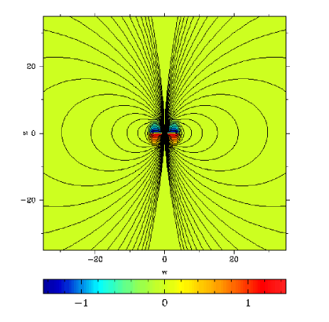
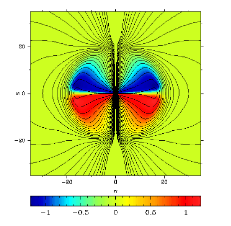
Figure 2: The evolution of spinned up dipole. This figure shows the solution at $t=5$ (left panel) and at $t=20$ (right panel). The contours show the magnetic flux function, $log_{10}\Psi$ and the colour image shows $H_{\phi}=2(I+I_{d})/c$, where $I$ is the electric current and $I_{d}$ is the displacement current.

4 MHD model

The difficulties that we have encountered in dealing with current sheets in force-free electrodynamics have forced us to return to the framework of full relativistic MHD even if the pulsar magnetospheres are expected to be magnetically dominated everywhere else and in spite of the fact that the system of MHD equations becomes stiff in this regime. The MHD approximation takes into account not only the gas pressure but also its inertia which may become important both far away from the star, in the wind zone, and near the light cylinder. Ideally we should also incorporate a physical model for electric resistivity which would allow us to conduct a proper study of the dissipation within the equatorial current sheet but it makes perfect sense to start with the simpler framework of ideal MHD.

4.1 Equations

The system of ideal relativistic MHD includes the continuity equation

$$\partial_{t}(\alpha\sqrt{\gamma}\rho u^{t})+\partial_{i}(\alpha\sqrt{\gamma}\rho u^{i})=0,$$ (24)

where $\rho$ is the rest mass density of matter and $u^{\nu}$ is its 4-velocity; the energy-momentum equations

$$\partial_{t}(\alpha\sqrt{\gamma}T^{t}_{\ \nu})+\partial_{i}(\alpha\sqrt{\gamma}T^{i}_{\ \nu})=\frac{1}{2}\partial_{\nu}(g_{\alpha\beta})T^{\alpha\beta}\alpha\sqrt{\gamma},$$ (25)

where $T^{\nu\mu}$ is the total stress-energy-momentum tensor; the induction equation,

$$(1/c)\partial_{t}(B^{i})+e^{ijk}\partial_{j}(E_{k})=0,$$ (26)

and the divergence free condition

$$\partial_{i}(\sqrt{\gamma}B^{i})=0.$$ (27)

The total stress-energy-momentum tensor, $T^{\mu\nu}$, is a sum of the stress-energy momentum tensor of matter

$$T_{(m)}^{\mu\nu}=wu^{\mu}u^{\nu}-pg^{\mu\nu},$$ (28)

where $p$ is the thermodynamic pressure and $w$ is the enthalpy per unit volume, and the stress-energy momentum tensor of the electromagnetic field

$$T_{(e)}^{\mu\nu}=\frac{1}{4\pi}\left(F^{\mu\gamma}F^{\nu}_{\ \gamma}-\frac{1}{4}(F^{\alpha\beta}F_{\alpha\beta})g^{\mu\nu}\right),$$ (29)

where $F^{\nu\mu}$ is the Maxwell tensor of the electromagnetic field. In the limit of ideal MHD

$$E_{i}=e_{ijk}v^{j}B^{k}/c,$$ (30)

where $v^{i}=u^{i}/u^{t}$ is the usual 3-velocity of plasma.

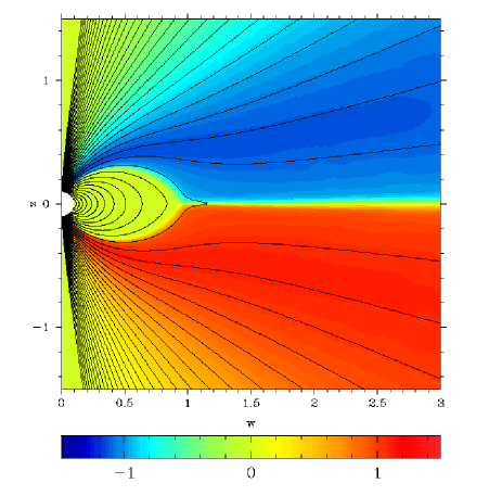
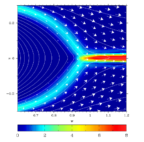
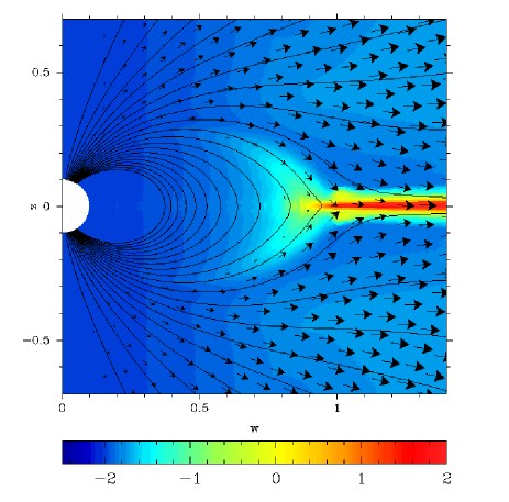
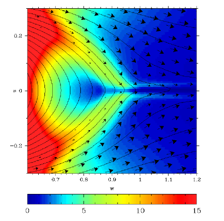
Figure 3: Inner part of the solution at $t=55$. Top left panel: The contours show the magnetic flux function, $\Psi$, and the colour image shows $H_{\phi}$; Top right panel: The contours show the magnetic flux function, $\Psi$, the arrows show the flow velocity, and the colour image shows the magnitude of the poloidal electric current density multiplied by $r^{2}$; Bottom left panel: The contours show the magnetic flux function, the arrows show the flow velocity, and the colour image shows the $\log_{10}(wW^{2}/B^{2})$; Bottom right panel: The contours show the magnetic flux function, the arrows show the flow velocity, and the colour image shows $B^{2}$.

4.2 Numerical method

The MHD simulations were carried out using a Godunov-type scheme that is described in Komissarov[Komissarov 1999, Komissarov 2004b]. However, we had to introduce a number of additional features in order to overcome a number of challenging problems specific to the case of highly-magnetized plasma.

The MHD equations become stiff in magnetically dominated domains and this is exactly the case for the main volume of pulsar magnetospheres where the energy density of matter is many orders of magnitude less than the one of the electromagnetic field. There is no hope of reaching such conditions with our numerical method. However, the electromagnetic part of the MHD solution should not be very different even when the energy ratio is artificially increased up to 0.1-0.01 – errors of order of few percent are quite acceptable at this stage of investigation. In fact, the results of force-free and MHD simulations of the monopole magnetospheres of black holes strongly support this conclusion [Komissarov 2001, Komissarov 2004b]. In those MHD simulations, additional plasma was pumped in the regions where its energy density had reached a certain lower limit. Here, we apply a similar trick. The actual condition is

$$wW^{2}\geq a_{(1)}B^{2},$$ (31)

where $W$ is the Lorentz factor of plasma and $a_{(1)}$ is a small constant (we used $a_{(1)}=0.01$.) When this condition is broken we increase both $\rho$ and $p$ in the same proportion so that $wW^{2}=a_{(1)}B^{2}$.

However, the dipolar magnetospheres are more challenging compared to the monopole ones because of the faster decline of magnetic field strength with the distance from the star and the existence of dead zones. Within the dead zones the magnetospheric plasma is supposed to be in static equilibrium. Thus, the component of the centrifugal force acting along the magnetic field lines has to be balanced by some other force. It has been argued that the dead zone plasma is charge-separated and the force balance is achieved by means of a small parallel component of electric field (e.g. [Holloway & Price 1981, Mestel 1999]). However the recent eclipse observations of the binary pulsar JO737-3039 allowed direct measurement of the particle density in the dead zone of one of the components [Lyutikov & Thompson 2005]. It has turned out to be many orders of magnitude higher than the expected density of the charged-separated plasma. Whether such a high density is specific for binary systems only, as proposed in [Lyutikov & Thompson 2005], or typical for single pulsars as well remains to be seen. In any case, the charge-separated dead-zones cannot be modelled within the MHD approximation where the required force balance can only be achieved by means of gas pressure. This would require the gas pressure to increase along the magnetic field line and reach a maximum in the equatorial plane. On the contrary, the magnetic pressure of dipolar magnetosphere decreases with distance as $r^{-6}$ and thus the ratio of magnetic to gas pressure has to decline even faster than $r^{-6}$. Given the requirement on the dead zone to remain magnetically dominated everywhere this implies very high pressure ratio near the star surface - much higher than our numerical scheme can accommodate. To overcome this problem one could consider the case where the star radius is only 2-3 times smaller than the radius of its light cylinder but this would have a rather strong effect on the structure of the magnetosphere. This is why we have preferred a different strategy.

Its idea is to reduce, somewhat arbitrarily, the dynamical effect of the centrifugal force on the motion of plasma near the star so that it does not destroy the nearly force-free equilibrium across the magnetic field lines within the dead zone. One way of achieving this is to reset the gas pressure and its rest mass density to some rather low ’target’ values, $p_{s}$ and $\rho_{s}$, within the dead zone every time step. At the same time one may reset the flow speed along the magnetic field lines to zero, just as it should be in equilibrium. However, the dead zone is not a well defined region in the case of time-dependent magnetospheres. Instead, one could apply the same procedure to a volume that is guaranteed to include if not the whole dead zone then at least its inner part. For example, we used a sphere of radius $r_{s}\leq\varpi_{lc}$. This however leads to another complication – in the open field region bounded by the sphere there emerges a strong rarefaction wave, so strong that the code crashes. Fortunately, this can be avoided if instead of resetting the target values one introduces a relaxation towards them with the relaxation time gradually increasing towards the boundary of the relaxation domain. We evolved $p$, $\rho$, and $\mn@boldsymbol{v}_{\parallel}$ according to the following equations

$$\frac{d\mn@boldsymbol{v}_{\parallel}}{dt}=-b_{(1)}\mn@boldsymbol{v}_{\parallel},$$ (32)

$$\frac{dp}{dt}=-b_{(2)}(p-p_{s}),$$ (33)

$$\frac{d\rho}{dt}=-b_{(2)}(\rho-\rho_{s}),$$ (34)

where

$$b_{(1)}(r)=b_{(0)}f(r),$$ (35)

$$b_{(2)}(r,\theta)=b_{(1)}|\cos\theta|,$$ (36)

$$f(r)=\left\{\begin{array}[]{rl}(r_{s}-r)/(r_{s}-r_{*})&\quad\mbox{if}\quad r<r_{s}\\ 0&\quad\mbox{if}\quad r>r_{s}\end{array}\right.,$$ (37)

where $b_{(0)}$ is constant, and $r_{*}$ is the star radius. As one can see, the relaxation time becomes infinite at $r=r_{s}$. The results presented below correspond to $r_{s}=\varpi_{lc}$. However, we have also tried smaller values of $r_{s}$ in order to verify that this does not lead to qualitatively different results (We discuss the effects of reducing $r_{s}$ in Section 5.) The dependence of $b_{(1)}$ on the azimuthal angle was introduce in order to reduce the possible adverse effect on the current sheet should it be formed inside the light cylinder. The actual value of $b_{(0)}$ is to be found by the method of trial and error. Finally, we use the following targets for the pressure and density

$$p_{s}=a_{(2)}\rho_{s}c^{2},\,\rho_{s}c^{2}=a_{(1)}B^{2},$$ (38)

where $a_{(1)}=0.01$ and $a_{(2)}=0.001$.

In these simulations, the computational grid covered the axisymmetric domain $(r,\theta)=[0.1,50]\times[0,\pi]$ and hence the star radius was set to $r_{*}=0.1$. In order to speed up the calculation we started with a relatively low resolution grid, $124\times 61$, and then increased the resolution twice after the solution seemed to have reached a steady-state on the scale of several $\varpi_{lc}$. Hence the final grid had $496\times 244$ cells.

4.3 Results

The initial solution described a non-rotating magnetosphere with dipolar magnetic field, eq.(3), $v^{i}=0$, $\rho=\rho_{s}$, and $p=p_{s}$. At $t=0$ the star rotation is switched on and a torsional Alfvén wave is emitted from its surface. As it propagates away larger and larger portion of the magnetosphere is set into rotation and develops an electric current system. This process is illustrated in figure 2 where the contours show the magnetic field lines and the colour image shows the distribution of $H_{\phi}=2(I+I_{d})/c$, where I is the total electric current and $I_{d}$ is the total displacement current through the circular contour of cylindrical radius $\varpi=r\sin\theta$. Unity corresponds to $H_{\phi}=\mu\Omega^{2}c^{-2}$.

Behind the wave the solution gradually approaches a steady state. Figure 3 shows the inner region of this steady state solution at $t=55$, the termination time of the simulations. The structure of magnetic field lines suggests that the dead zone extends all the way up to the light cylinder. Beyond the light cylinder the poloidal magnetic field becomes radial, as expected [Ingraham 1973, Michel 1974]. Some magnetic field lines are closing up beyond the light cylinder but they do so within the equatorial current sheet due to finite artificial resistivity in the numerical scheme – it is easy to see the transition between the dead zone and the current sheet within which the magnetic field lines are highly stretched in the radial direction. The colour image in the top left panel of this figure shows the distribution of $H_{\phi}$. Since in a steady state the displacement current vanishes we have $H_{\phi}=2I/c={\cal A}.$ This image confirms our conclusion on the extension of the dead zone which is seen in the image as a toroidal structure with $H_{\phi}=0$ (Indeed, within the dead zone the poloidal currents do not flow and $H_{\phi}$ must be zero.) The jumps in $H_{\phi}$ occurring at the boundary of the dead zone and along the equator are indicators of thin sheets of return current. This image also shows, though not as clear, that $H_{\phi}$ and hence $I$ reach maximum amplitude at some finite distance from the equatorial plane. This indicates the presence of an additional layer of return current that surrounds the equatorial current sheet and the dead zone [Contopoulos et al. 1999].

The current sheets are most prominent in the right panel of figure 3 that shows the distribution the poloidal current density, $\mn@boldsymbol{J}_{p}$, multiplied by $r^{2}$. One can also see that the thickness of the current sheets near the Y-point is about $0.5\div 0.6\varpi_{lc}$ and that equatorial current sheet extends inside the light cylinder by approximately the same distance.

Figure 4: $H_{\phi}$ as a function of the magnetic flux function $\Psi$ on the sphere $r=1.1$ at time $t=55$.

From time to time it was suggested that particle inertia may actually become dynamically important near the light cylinder, thus rendering the force-free approximation as unsuitable. The argument develops like this. Provided the magnetospheric plasma simply co-rotated with the star its speed would exceed the speed of light beyond the light cylinder. This does not occur because of the rapidly increasing inertial mass of this plasma near the light cylinder. This leads to very strong centrifugal force that makes the plasma to flow across the light cylinder thus opening up the magnetic field lines and sweeping them back. However, this not what occurs in our simulations. Indeed, the top left panel of figure 3 shows that, very much in agreement with the force-free models, $H_{\phi}$ is constant along the magnetic flux surfaces even when they cross the light cylinder. Moreover, this conclusion is fully supported by the data presented in the bottom left panel of figure 3 that shows that the distribution of $wW^{2}/B^{2}$, the quantity that can be used to describe the relative importance of the inertial effects as well as of the gas pressure. One can see that it remains very low everywhere outside of the equatorial current sheet including the light cylinder.

There is, however, one location in the force-free solution of Contopoulos et al.[Contopoulos et al. 1999] where the inertial effects are expected to become important. It is the so-called Y-point, that is the point where the dead zone approaches the light cylinder. Indeed, since the dead zone co-rotates with the star then plasma particles attached to its field lines rotate with the speed reaching the speed of light at the y-point. Moreover, one may argue that the divergence of magnetic field strength at the Y-point discovered by Gruzinov[Gruzinov 2005] also suggests a breakdown of the force-free approximation. This fully agrees with the data presented in the bottom right panel of figure 3 which shows the distribution of $B^{2}$ in our MHD solution. Although the plot shows a local minimum at $(z,\varpi)=(0,0.85)$ and then some growth of $B^{2}$ in the direction of the Y-point this growth never develops. Moreover, in our solution the poloidal magnetic field lines approach the Y-point at an angle of $\simeq 50^{o}$ to the equatorial plane (see fig.3), which is significantly lower than $77^{o}.3$ predicted by Gruzinov[Gruzinov 2005] and quite close to the value of $56^{0}.5$ found in Goodwin et al.[Goodwin et al. 2004]. In addition to the inertial effects, the relatively high thickness of the current sheets near the Y-point (the right top panel of figure 3) and finite gas pressure also contribute to these discrepancies between our simulations and the force-free solution. Our results however do not prove that the asymptotic force-free solution for the Y-point is irrelevant. It seems possible that for sufficiently high magnetization and small resistivity the exact MHD solution will first approach the force-free asymptote found by Gruzinov and then deviate from it on smaller scales. This, however, requires further investigation.

Figure 5: Left panel: The magnetic flux function, $\Psi$, in the equatorial plane as a function of $r$ at time $t=55$. Right panel: The total energy flux through a sphere of radius $r$ at time $t=55$.

Figure 6: The angular velocity distribution at $t=55$ within the light cylinder at $r=0.2$ (left panel) and at $r=0.7$ (right panel). The dot-dashed, dashed, and solid lines show the solutions with 61, 122, and 244 cells in the $\theta$-direction.

Figure 4 shows $H_{\phi}$ as a function of $\Psi$ at $r=1.1$ and allows us to see these details of the current system more clearly. This distribution is very similar to the one given in figure 4 of Contopoulos et al. (1999). The minimum has

$$\Psi_{min}\simeq 1.02\frac{\mu\Omega}{c}\quad\mbox{and}\quad A_{min}\simeq 1.12\frac{2\mu\Omega^{2}}{c^{2}}.$$

The left panel of figure 5 shows the distribution of magnetic flux function $\Psi$ in the equatorial plane of the final solution. As a consequence of the finite artificial resistivity in our numerical scheme the magnetic field lines continue to close up even beyond the line cylinder and this shows itself via a systematic decline of $\Psi$ at $r>1$. Thus, it is not so straightforward to determine the fraction of opened field lines in this solution. One way to describe it quantitatively is by giving the value of the flux function exactly at $(\theta=\pi/2,r=1)$. This gives us

$$\Psi_{yp}\simeq 1.37\div 1.38\frac{\mu\Omega}{c}.$$ (39)

On the other hand, figure 5 shows that the decline of $\Phi$ significantly slows down at $r>2$ where $\Phi$ reaches the value of

$$\Psi_{open}\simeq 1.26\div 1.27\frac{\mu\Omega}{c}.$$ (40)

These numbers should be compared with the $c\Psi_{open}/\mu\Omega=1.23$ in Contopoulos[Contopoulos 2005] and Timokhin[Timokhin 2005], $1.27$ in Gruzinov[Gruzinov 2005], and $1.36$ in Contopoulos et al.[Contopoulos et al. 1999].

The right panel of figure 5 shows the total flux of energy through the sphere of radius $r$ that should be constant in a steady state solution. One can see that it is indeed more or less constant with the exception of $1<r<2$ where the energy flux slightly increases. This increase is a permanent feature that arises because our scheme is not strictly conservative. In order to evaluate the spin-down power of the star we used the energy flux through the sphere of radius $r=1$, thus ignoring the non-physical increase of total luminosity beyond $r=1$. This gives us

$$L\simeq 1.1\frac{\mu^{2}\Omega^{4}}{c^{3}}$$ (41)

which is in a very good agreement with the result by Gruzinov(2005).

Figure 6 shows the distribution of the angular velocity of magnetic field lines, $\Omega_{f}$. In the exact steady-state force-free solution the magnetic field lines rotate with same angular velocity as the star,

$$\Omega_{f}=\Omega.$$ (42)

However in our solution, $\Omega_{f}$ noticeably deviates from $\Omega$ inside the layer coincident with the current sheet between the open field lines and the dead zone (see fig.6). The most likely reason for this is the enhanced numerical resistivity in the current sheet. The comparison of solutions with different numerical resolution (fig.6) shows that the thickness of the layer significantly decreases with resolution. However, the amplitude of the perturbations does not seem to depend on the resolution.

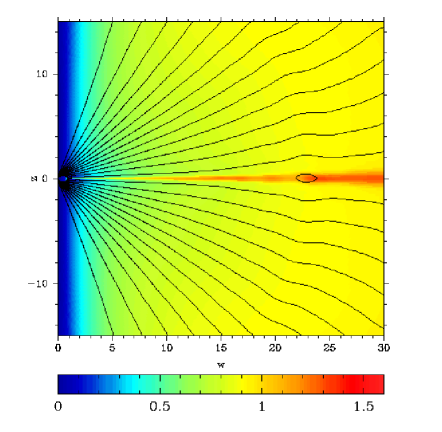
Figure 7: The wind zone structure of a dipolar magnetosphere. The contours show the field lines of poloidal magnetic field. The colour image shows the distribution of $\log_{10}W$

Figure 8: The variation of a number key parameters along the ray $\theta=1$. Left panel: The local magnetization parameter $\tilde{\sigma}$; Middle panel: The wavespeed of the ingoing fast wave in the radial direction (the speed of light c=1); Right panel: The Lorentz factor of the wind.

Figure 7 shows that far away from the star the distribution of poloidal field lines is very similar to the split-monopole one. This is exactly what was concluded in the pioneering papers by Ingraham[Ingraham 1973] and Michel[Michel 1974] on the force-free magnetospheres. More recently, the centrifugally driven outflows in split-monopole magnetospheres have been studied within the cold-MHD approximation. According to these studies the Lorentz factor of centrifugally accelerated plasma at the fast critical point is

$$W=\sigma^{1/3},$$ (43)

where $\sigma$ is the so-called magnetization parameter which is defined as the ratio of the Poynting flux density to the rest mass-energy flux density at the foot point of the magnetic field line [Beskin 1997]. For outflows that are initially Poynting dominated $\sigma\simeq\tilde{\sigma}$, where $\tilde{\sigma}$ is the ratio of the total energy flux density to the rest mass-energy flux density. In contrast to $\sigma$, $\tilde{\sigma}$ can be measured at every point of the field line as it is constant along it. Figure 8 shows the distribution of $\tilde{\sigma}$, $W$, and the ingoing speed of the fast wave in the radial direction along the ray $\theta=1$rad. From these data we find that along this ray $\sigma\simeq 77$ and the fast point is located at $r\simeq 6.8$ where $W\simeq 4.3$. On the other hand, we can use the above value of $\sigma$ in order to calculate the Lorentz factor at the fast point directly from eq. 43 – this give us $W=4.25$. Thus, the split-monopole model provides quite a good model for the wind zone of aligned magnetic dipole.

Another interesting feature of figure 7 is the significantly higher value of the Lorentz factor of the outflow within the equatorial current sheet. This suggests that the mechanism of the flow acceleration is somewhat different there. The obvious suspect is heating due to resistive dissipation of the electromagnetic energy. The high value of Lorentz factor in the current sheet suggests that its contribution into the global energy transfer can be quite significant.

The left panel of figure 9 shows the evolution of the wind luminosities with the distance from the star by the end of simulations. The total luminosity is more or less constant apart from noticeable perturbations around $r=17$, $r=30$, and $r=45$. The big bump around $r=45$ is related to the leading front of the wind. The perturbations around $r=17$ and $r=30$ are related to the grid refinement events – each time the computational grid is refined the numerical solution evolves to a slightly different state, most of all in the inner region of the computational domain. This triggers noticeable waves propagating away from the star. The electromagnetic luminosity, which is shown in figure 9 by the dashed line, gradually decreases with distance thus indicating the ongoing conversion of the electromagnetic energy into the hydrodynamic energy. This is supported by the evolution of the hydrodynamic luminosity of the wind which is shown by the dash-dotted line. One of the interesting feature of this line is its rapid rise initial rise that suggests a particularly effective energy conversion. The nature of this conversion is clarified in the right panel of figure 9 that shows that the current sheet accounts for about 70% of the total hydrodynamic luminosity at $r=10$ and this corresponds to about 15% of the total wind luminosity. This clearly points out at the Ohmic heating in the current sheet as the main source of the energy conversion.

Figure 9: Conversion of the electromagnetic luminosity into the hydrodynamic luminosity of the wind. Left panel: The total luminosity (solid line), the electromagnetic luminosity (dashed line), and the hydrodynamic luminosity (dot-dashed) of the wind at $t=55$. Right panel: The angular distribution of the total luminosity at $r=10$. The solid line and the dot-dashed line show the total luminosity and the hydrodynamic luminosity within the polar cone of angle $\theta$ respectively; the dashed line shows the total flux density in the radial direction.

5 Discussion

There is not much to discuss in connection with our force-free simulations of pulsar magnetospheres. We simply have not been able to make the required progress using this framework because of the inability to handle the equatorial current sheet. For this reason we will focus in this section almost entirely on the results of our MHD simulations and their possible implication for pulsar physics.

One of the key goals of this study was to determine there the MHD equations allow stable, or quasi-stable, steady-state solutions for dipolar axisymmetric magnetospheres of neutron stars. This problem had become particularly interesting since the discovery a whole family of steady-state force-free solutions continuously parametrised by the location of their y-point [Goodwin et al. 2004, Timokhin 2005]. Our results indicate the existence of a unique steady-state MHD solution to the problem and this solution is very close to the force-free stationary solution of the pulsar equation with the y-point located at the light cylinder – the original solution of pulsar found by Contopoulos et al.[Contopoulos et al. 1999]. Why this solution is preferable to those whose y-point is located well inside the light cylinder has already been explained in [Contopoulos 2005]. If resistivity is not vanishingly small then even if the initial solution had the dead zone buried well inside the light cylinder it would take only a finite time for the anti-parallel field lines of the current sheet between the y-point and the light cylinder to reconnect and to form closed loops that become a part of the dead zone. The reconnection should also occur beyond the light cylinder but there the outflow is super-Alfvénic so the net outcome of the reconnection is likely to be the development of magnetic islands carried by the wind away from the star [Uzdensky 2004]. The rate of the reconnection depends on the actual resistivity in the current sheet, and in our simulations the resistivity is purely artificial. However, the ultimate outcome is unlikely to be different. Indeed, since the particle inertia on the closed field lines located well inside the light cylinder of pulsar magnetospheres is extremely small there is no restoring force that would make this field lines to open up again. This is supported by the fact that the total electromagnetic energy of the force-free magnetosphere is minimum when the Y-point is located on the light cylinder [Timokhin 2005].

At this point it makes sense to discuss whether the relaxation procedure applied within $r_{s}=\varpi_{ls}$ (see Sec.4.2) could somehow promote the expansion of the dead zone towards the light cylinder. As we have already pointed out in Sec.4.2 all relaxation times gradually increase towards infinity as $r\rightarrow r_{s}$. Thus, near the light cylinder the effect of the relaxation procedure on the flow is increasingly small. Moreover, the relaxation time for the gas pressure becomes infinite at $\theta=\pi/2$. This would allow the build up of gas pressure required to support the equatorial current sheet should it exist within the light cylinder. However, in order to fully resolve this issue we carried out additional simulations with the radius of the relaxation sphere pushed down to $r_{s}=0.7\varpi_{lc}$. Figure 10 allows to compare both solutions with regard to the location of the Y-point. The colour image in this figure shows the distribution of $H_{\phi}$ and the solid lines show the magnetic surfaces for the model with $r_{s}=0.7\varpi_{lc}$ whereas the dashed lines show the magnetic surfaces for the model with $r_{s}=\varpi_{lc}$. As one can see more field lines open up for smaller $r_{s}$ and this is caused by the increased dynamical role of the centrifugal force. However, the location of Y-point remains basically the same. Thus, our relaxation procedure cannot be considered as the reason for the dead zone extending all the way up to the light cylinder.

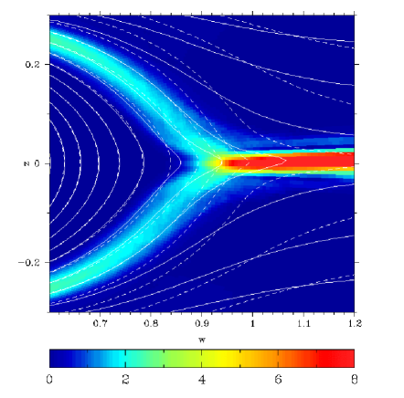
Figure 10: Comparison of solutions with relaxation domains of different sizes. The colour image shows $H_{\phi}$ and the solid lines show the magnetic flux function for the model with $r_{s}=0.7\varpi_{lc}$. The dashed lines show the magnetic flux function for the model with $r_{s}=\varpi_{l}$.

Contopoulos[Contopoulos 2005] also pointed out that the open field lines of pulsar magnetospheres may rotate at a slower rate than the closed field lines of the dead zone due to the finite potential gap of the polar cap. In particular, he speculated about the possibility of a significant growth of the polar gap due to a sudden decrease of the particle injection rate in the gap in order to explain the explosive phenomena like the December 27, 2004 burst in SGR 1806-20. Although, it is not clear what could cause such a sudden incident of “charge starvation” it was suggested long ago that a slow systematic evolution of the polar gap could result from the gradual spin-down of the star [Sturrock 1971, Ruderman & Sutherland 1975]. Thus, differentially rotating magnetospheres are not just interesting theoretical models but can be very much relevant for the real pulsars.

Contopoulos[Contopoulos 2005] found force-free stationary numerical solutions for such magnetospheres in the simple case of a uniformly rotating polar cap and a uniformly rotating dead zone which was assumed to corotate with the star. (In fact, the dead zone may also have a potential gap that separates electric charges of opposite sign but it is expected to be rather small [Holloway & Price 1981].) These solutions have two light cylinders – a smaller one for the dead zone and and a larger one for the open field lines and the dead zone extends all the way up to its light cylinder. Contopoulos[Contopoulos 2005] argued that although there existed solutions with a smaller dead zone they were not sustainable due to reconnection in the part of the equatorial current sheet that runs between the y-point and the light cylinder of the dead zone.

In fact, the numerical models constructed by Contopoulos[Contopoulos 2005] are likely to be globally unstable to reconnection too. Indeed, in these models the equatorial current sheet continues inside the light cylinder of open magnetosphere and magnetic reconnection occurring in this region should lead to creation of new closed field lines. However, this case is somewhat more involved. Let us imagine that such reconnection has indeed occurred. The field lines that have just closed down are now beginning to spin-up and corotate with the dead zone. However, they extend beyond the light cylinder of the dead zone and for this reason they can not corotate with it – as they spin-up they begin opening up again. Once have been opened up they begin to slow down, thus creating conditions for the next closing down event, and so on. This simple analysis suggests that such differentially rotating magnetospheres cannot be stationary and have to develop oscillations. The typical time scale of such magnetospheric oscillations seems to be determined by the spin-up time that must be comparable with the time required for an Alfvén wave to cross the distance between the light cylinder of the dead zone and the star back and forward. Since the Alfvén speed is relativistic and the magnetic field has a significant radial component the crossing time has to be comparable with with rotational period of the star. The reconnection rate is more likely to effect the amplitude of these oscillations rather than their time-scale, a quicker reconnection leading to a larger fraction of magnetic field lines involved in this process of closing down and opening up. We wont to speculate that these oscillations may be relevant to the origin of the sub-pulses of radio pulsars, e.g. [Manchester & Taylor 1977]. For periodic magnetospheric oscillations we would have a phenomena reminiscent of beating waves – this may explain the so-called drifting sub-pulses. However, one may also expect quasi-periodic and even chaotic oscillations and they would results in a much more complicated behaviour of sub-pulses.

Our MHD solution has a number of interesting features that could not possibly be found in the ideal force-free solution of Contopoulos et al.(1999). Some of them do not depend much on the details of resistivity like, for example, the centrifugal acceleration of the wind outside of the current sheet. Others, like the Ohmic dissipation and the wind acceleration in the equatorial current sheet, do and we have to exercise a reasonable degree of caution when interpreting them – MHD simulations with only artificial resistivity can provide at most qualitatively correct description of such features. However, it is interesting that the dissipation of electromagnetic energy in the equatorial current sheet has already been considered as a promising explanation of the high luminosity gamma-ray emission from young pulsars [Lyubarskii 1996, Kirk et al. 2002]. Given the fact that these gamma-rays carry away a significant fraction of the spin-down power, up to 10% in the most extreme examples [Thompson 2001], and that pulsar magnetospheres are highly magnetically dominated, an efficient dissipation of Poynting flux somewhere in the magnetosphere is needed to explain these observations, and the equatorial current sheet is one of the most natural locations for such dissipation. In particular, Lyubarskii (1996) argued that this high energy emission originates from the current sheet just beyond the dead zone (This is exactly where our simulations show most effective Ohmic dissipation.) The polarizational observations of the optical emission from the Crab pulsar support this idea. This emission is found to be polarised parallel to the rotation axis at the peaks of the pulses and between the pulses (within the pulses the polarisation vector rotates, which may be attributed to the rotation of the magnetosphere). This shows that the magnetic field of the emitting region is predominantly perpendicular to the rotation axis as it should be if this radiation is generated in the equatorial current sheet.

References

- [Asano et al. 1999] Asano E., Uchida T., Matsumoto R., 2005, Publ.Astron.Soc.Jpn., 57, 409-413.
- [Beskin 1990] Beskin V.S., 1990, Sov.Astron.Lett., 16(4), 286.
- [Beskin 1997] Beskin V.S., 1997, Physic-Aspect, 40, 659.
- [Beskin 2005] Beskin V.S., Axisymmetric flows in Astrophysics, Moscow, 2005.
- [Beskin et al. 1993] Beskin V.S., Gurevich A.V., Istomin Ya.N., 1993, Physics of the Pulsar Magnetosphere, Cambridge University Press, Cambridge.
- [Contopoulos et al. 1999] Contopoulos I., Kazanas D., Fendt C., 1999,ApJ,511,351.
- [Contopoulos 2005] Contopoulos I., 2005, astro-ph/0507201.
- [Goodwin et al. 2004] Goodwin S.P., Mestel J., Mestel L., Wright A.E., 2004, MNRAS,349,213.
- [Gruzinov 1999] Gruzinov A., 1999, preprint, astro-ph/9902288.
- [Gruzinov 2005] Gruzinov A., 2005, Phys.Rev.Lett., 94, 021101.
- [Hibschman & Arons 2001] Hibschman J.A. and Arons J., 2001, ApJ, 546, 382.
- [Holloway & Price 1981] Holloway N.J. and Pryce M.H.L., 1981, MNRAS, 194, 95.
- [Ingraham 1973] Ingraham, R. L., 1973, ApJ, 186, 625
- [Kirk et al. 2002] Kirk J.G., Skjæraasen O. and Gallant Y.A., 2002, A&A, 388,L29.
- [Komissarov 1999] Komissarov S.S., 1999, MNRAS, 303, 343.
- [Komissarov 2001] Komissarov S.S., 2001, MNRAS, 326, L41.
- [Komissarov 2002a] Komissarov S.S., 2002a, MNRAS, 336, 759.
- [Komissarov 2002b] Komissarov S.S., 2002b, in the proceedings of The 3rd International Sakharov Conference on Physics held in Moscow, Russia, June 24-29, 2002, eds A.Semikhatov, M.Vasiliev, V.Zaikin, Scientific World Publishing Co., p.392-400; (astro-ph/021114).
- [Komissarov 2004a] Komissarov S.S., 2004a, MNRAS, 350,427.
- [Komissarov 2004b] Komissarov S.S., 2004b, MNRAS, 350, 1431.
- [Komissarov & Lyubarsky 2004b] Komissarov S.S., Lyubarsky Y.E., 2004, MNRAS, 349, 779.
- [Kanbach et al. 2003] Kanbach G., Kellner S.,Score F.Z., Straubmeier C., and Spruit H.C., 2003, in Instrument Design and Performance for Optical/Infrared Ground-based Telescopes, Editors: Iye M, Moorwood AFM, Proceedings of SPIE, 4841, pp.82-93.
- [Lyubarskii 1990] Lyubarskii Y.E., 1990, Sov.Astron., 16,16.
- [Lyubarskii 1996] Lyubarskii Y.E., 1996, A&A, 311,72.
- [Lyutikov 2003] Lyutikov M., 2003, MNRAS, 346,540.
- [Lyutikov & Thompson 2005] Lyutikov M., Thompson C., 2005, astro-ph/0502333.
- [Manchester & Taylor 1977] Manchester R.N and Taylor J.H., Pulsars, W.H.Freeman and Company, San Francisco, 1977.
- [Mestel 1999] Mestel L., 1999, Stellar Magnetism, Clarendon Press,Oxford.
- [Michel 1973] Michel F.C., 1973, ApJ, 180, L133.
- [Michel 1974] Michel F.C., 1974, ApJ, 187, 585.
- [Michel 1982] Michel F.C., 1982, Rev.Mod.Phys.,54, 1.
- [Muslimov & Tsygan 1990] Muslimov A.G. and Tsygan A.I., 1990,Sov.Astron., 34,133.
- [Petri & Kirk 2005] Petri J. and Kirk J., 2005, astro-ph/5427.
- [Punsly 2001] Punsly B., 2003, ApJ, 583, 842.
- [Ruderman & Sutherland 1975] Ruderman M.A. and Sutherland P.G., 1975, ApJ,196,51.
- [Scharlemann & Wagoner 1973] Scharlemann, E.T., Wagoner, R.V. 1973, ApJ,182, 951
- [Spitkovsky 2004] Spitkovsky A., in F.Camilo and B.M.Gaensler (eds) Young neutron stars and their environments IAU Symposium, v.218, 2004.
- [Sturrock 1971] Sturrock P.A., 1971,ApJ,164, 529.
- [Thompson 2001] Thompson D.J., 2001, in Felix A. Aharonian and Heinz J. Völk (eds.), High Energy Gamma-Ray Astronomy, American Institute of Physics (AIP) Proceedings, Melville, New York, v.558, p.103.
- [Timokhin 2005] Timokhin A., 2005, astro-ph/0507054.
- [Uchida 1997] Uchida T., 1997, Phys.Rev.E, 56(2), 2181.
- [Uzdensky 2003] Uzdensky D.A., 2003, ApJ, 598,446.
- [Uzdensky 2004] Uzdensky D.A., 2004, Ap&SS, 292,573.