Evidence for alignment of the rotation and velocity vectors in pulsars

Abstract

We present strong observational evidence for a relationship between the direction of a pulsar’s motion and its rotation axis. We show carefully calibrated polarization data for 25 pulsars, 20 of which display linearly polarized emission from the pulse longitude at closest approach to the magnetic pole. Such data allow determination of the position angle of the linear polarisation which in turn reflects the position angle of the rotation axis. Of these 20 pulsars, 10 show an offset between the velocity vector and the polarisation position angle which is either less than 10° or more than 80°, a fraction which is very unlikely by random chance. We believe that the bimodal nature of the distribution arises from the presence of orthogonal polarisation modes in the pulsar radio emission. In some cases this orthogonal ambiguity is resolved by observations at other wavelengths so that we conclude that the velocity vector and the rotation axis are aligned at birth. Strengthening the case is the fact that 4 of the 5 pulsars with ages less than 3 Myr show this relationship, including the Vela pulsar. We discuss the implications of these findings in the context of the Spruit & Phinney (1998) model of pulsar birth-kicks. We point out that, contrary to claims in the literature, observations of double neutron star systems do not rule out aligned kick models and describe a possible observational test involving the double pulsar system.

1 Introduction

The velocities of pulsars are significantly larger than those of their progenitor (high-mass) stars (e.g. Lyne & Lorimer 1994). This implies that the birth process of pulsars also produces their high velocities and that the supernova or events soon thereafter must be asymmetrical. The mechanisms driving this asymmetry are far from clear. Tademaru & Harrison (1975) proposed the so-called rocket mechanism whereby an offset of the magnetic dipole from the centre of the star causes the star to accelerate along its rotation axis. Observational tests of this mechanism by Morris, Radhakrishnan & Shukre (1976) and Tademaru (1977) reached opposing conclusions, with the former claiming no correlation between the velocity vector and the spin axis, and the latter claiming a good correlation. Following this, Anderson & Lyne (1983) revisited the issue with an updated database of pulsar proper motions. They also saw no apparent alignment between the proper motion angle and the rotation axis although they included many old pulsars in their sample, whose direction of motion may have significantly evolved in the Galactic potential. In the late 1980s, a group of papers concentrated mainly on asymmetric explosions and the break-up of binary systems as the origin for pulsar velocities [Radhakrishnan & Shukre 1986, Dewey & Cordes 1987, Bailes 1989] and the rocket model fell out of favour.

A decade later, the debate started anew when Spruit & Phinney (1998) and Cowsik (1998) proposed a model in which the same (off-centre) explosion processes that give pulsars their high velocity also produce their fast rotation. Although their models were motivated by theoretical results suggesting that the pre-supernova stellar configuration is not spinning quickly enough to account for birth periods of $\sim$10 ms from conservation of angular momentum alone, the basic physics applies - any significant off-centre impulses would both accelerate and torque the pulsar. In the Spruit & Phinney (1998) model, a single, short-duration impulse leads to the rotation axis being perpendicular to the velocity vector. However, even a few short duration kicks as the star spins serve to destroy this correlation. They also considered kicks of finite duration ($\geq$ the spin period) and showed in this case that the rotation axis should be parallel with the velocity vector. Deshpande, Ramachandran & Radhakrishnan (1999) tested these ideas by using the literature to search for pulsars which had accurate proper motion measurements and good polarization observations. They used the polarization measurements to determine the point of inflexion of the PA sweep although give no details as to how this was done. They took the associated position angle as the angle of the rotation axis on the sky (or, to allow for orthogonal mode emission, its orthogonal). In their sample of 29 pulsars they saw no statistical evidence for any correlation between the velocity vector and the rotation axis. In the context of the Spruit & Phinney (1998) model they favoured multiple short duration impulses as the origin of the spin and velocity kicks.

Observational evidence for a correlation between the spin axis and the proper motion next came from an unexpected source. Helfand et al. (2001) showed high resolution X-ray images of the Vela pulsar and its surrounding nebula. Two prominent arcs are seen, which Helfand et al. (2001) interpret as originating from the front surface of an equatorial wind whose axis of symmetry is the rotation axis of the pulsar. The position angle of the axis of this torus is 130° and 310°. The axis of the torus, created by pulsar winds, is likely aligned with the pulsar rotation axis. Helfand et al. (2001) then note that the position angles of the torus and pulsar spin axes are within 10° of the proper motion vector of 301° obtained by Dodson et al. (2003). Following from the Vela result, X-ray imaging of a number of young pulsars showed that many had pulsar wind nebulae consisting of an equatorial torus and polar jets. Ng & Romani (2004) used this information to determine the angle of rotation axis on the plane of they sky and compared this to the velocity vector if available. For the Crab and Vela pulsars these clearly matched but there was also good evidence for a match in the other pulsars in their sample (PSRs J0538+2817, B1951+32 and B1706–44). It appears likely from this study that the directions of motion of young pulsars lie along the rotation axes, although their sample is small.

Historically, the velocity vectors of pulsars have been measured either through proper motion measurements using Very Long Baseline Interferometry (VLBI) techniques or through highly accurate timing. The first method tends to be possible only for relatively nearby pulsars, whereas the second method was generally restricted to millisecond pulsars which show almost no intrinsic timing jitter. Recently, however, Hobbs et al. (2004) have shown that it is possible to measure proper motions of pulsars even in the presence of timing noise. In brief, this involves very long (tens of years) timing sets coupled with a ‘whitening’ technique to remove the timing noise. Using this method, Hobbs et al. (2004) list proper motion measurements for 302 pulsars. Updates to these parameters and a catalogue of the best available proper motions from either timing or interferometry are available in Hobbs et al. (2005) and in particular provide celestial position angles (PA_v) of the velocity vectors.

In the absence of external features such as pulsar wind nebulae and tori, the position angle of the axis of rotation (PA_r) of a pulsar has to be determined from polarisation observations using a several-step procedure. One first has to determine PA₀, the position angle of polarization at the point of closest approach of the observer’s line of sight to the magnetic pole. This angle must then be corrected for Faraday rotation in the interstellar medium and the ionosphere in order to reflect the true angle at the pulsar. Determination of PA₀ itself is difficult. We discuss two techniques.

In the rotating vector model (RVM) of Radhakrishnan & Cooke (1969), the radiation is beamed along the field lines and the plane of polarization is determined by the angle of the magnetic field as it sweeps past the line of sight. The PA as a function of pulse longitude, $\phi$, can be expressed as

$${\rm PA}={\rm PA}_{0}+{\rm arctan}\left(\frac{{\rm sin}\alpha\,{\rm sin}(\phi-\phi_{0})}{{\rm sin}\zeta\,{\rm cos}\alpha-{\rm cos}\zeta\,{\rm sin}\alpha\,{\rm cos}(\phi-\phi_{0})}\right)$$ (1)

Here, $\alpha$ is the angle between the rotation axis and the magnetic axis, where $\zeta=\alpha+\beta$, $\beta$ being the angle at closest approach of the line of sight to the magnetic axis. $\phi_{0}$ is the corresponding pulse longitude at which the PA is then PA₀. Unfortunately, for most pulsars it is difficult to determine $\alpha$ and $\beta$ with any degree of accuracy, partly because the longitude over which pulsars emit is rather small and partly because strong deviations from a simple swing of PA are often observed. This makes the determination of PA₀ straightforward only in the $\sim$15 per cent of pulsars for which the RVM works (see also Everett & Weisberg 2001).

Figure 1: Geometry of the pulsar beam and velocity vector as seen by the observer. The observer sees a projection of the direction of the rotation axis, PA_r, and the velocity vector, PA_v, onto the plane-of-the sky shown on the right. The angle $\alpha$ is the inclination angle of the magnetic and rotation axis, while $\beta$ is the impact parameter between the magnetic axis and the line-of-sight at closest approach. The vector PA_∥ lies along the field line in this fiducial plane ($\phi_{0}$) and hence has the same value as PA_r. PA_⟂ lies orthogonal to the magnetic field at closest approach. In the absence of other information we do not know whether the observed PA₀ corresponds to PA_∥ or PA_⟂. Note that PA_∥ and PA_⟂ (and hence PA_r) have 180° ambiguities inherent to all polarization measurements, unlike PA_v.

Table 1: Proper motions, rotation measures and polarisation position angles for a sample of 25 pulsars.

		Age	Dist	Proper Motion				Rotation Measure			Poln
Jname	Bname	log($\tau_{c}$)		$\mu_{\alpha}$	$\mu_{\delta}$	Ref	PAv	Previous	Ref	Measured	PA0
		(yr)	(kpc)	(mas/yr)	(mas/yr)		(deg)	(rad m-2)		(rad m-2)	(deg)
J0525+1115	B0523+11	7.9	3.1	27(2)	$-$24(10)	1	132(16)	35(3)	1	37(2)	$-$65(4)
J0601$-$0527	B0559$-$05	6.7	3.9	$-$5(3)	$-$20(6)	1	194(16)	67(5)	2	62.4(20)	—
J0630$-$2834	B0628$-$28	6.4	1.4	$-$44.6(9)	19.5(22)	2	294(3)	46.19(9)	3	46.53(12)	26(2)
J0742$-$2822	B0740$-$28	5.2	2.1	$-$29(2)	4(2)	3	278(5)	156(5)	4	149.95(5)	$-$81.7(1)
J0820$-$1350	B0818$-$13	7.0	2.0	18(3)	$-$46(5)	1	159(6)	$-$1.2(4)	3	$-$7.2(12)	65(2)
J0835$-$4510	B0833$-$45	4.1	0.29	$-$49.60(6)	29.8(1)	4	301.0(1)	38.17(6)	5	31.38(1)	36.8(1)
J0908$-$1739	B0906$-$17	7.0	0.9	22(3)	$-$94(4)	1	167(2)	$-$36(6)	2	$-$31(4)	—
J0922+0638	B0919+06	5.7	1.2	18.35(6)	86.56(12)	5	12.0(1)	32(2)	2	29.2(3)	—
J0953+0755	B0950+08	7.2	0.26	$-$2.09(8)	29.46(7)	6	355.9(2)	1.35(15)	3	$-$0.66(4)	14.9(1)
J1136+1551	B1133+16	6.7	0.36	$-$74.0(4)	368.1(3)	6	348.6(1)	3.9(2)	6	1.1(2)	$-$78(2)
J1239+2453	B1237+25	7.4	0.86	$-$106.82(17)	49.92(18)	6	295.0(1)	$-$0.33(6)	3	$-$2.6(4)	$-$66(1)
J1430$-$6623	B1426$-$66	6.7	1.0	$-$31(5)	$-$21(3)	7	236(9)	$-$12(3)	3	$-$19.2(3)	$-$28.5(7)
J1453$-$6413	B1449$-$64	6.0	2.1	$-$16(1)	$-$21.3(8)	7	217(3)	$-$22.3(14)	3	$-$18.6(2)	$-$56.9(4)
J1456$-$6843	B1451$-$68	7.6	0.45	$-$39.5(4)	$-$12.3(3)	8	252.7(6)	$-$2(3)	3	$-$4.0(3)	$-$31.6(6)
J1645$-$0317	B1642$-$03	6.5	1.1	$-$3.7(15)	30.0(16)	2	353(3)	15.8(3)	3	17(2)	56(4)
J1709$-$1640	B1706$-$16	6.2	0.8	$-$9(3)	$-$44(21)	1	192(16)	$-$1.3(3)	2	$-$2(5)	15(2)
J1709$-$4429	B1706$-$44	4.2	2.3				160(10)	$-$7(4)	7	0.70(7)	—
J1740+1311	B1737+13	6.9	1.5	$-$21.5(22)	$-$19.7(22)	2	228(6)	64.4(16)	1	65(2)	$-$46(4)
J1844+1454	B1842+14	6.5	2.2	18(4)	25(7)	1	36(15)	121(8)	2	109.0(13)	$-$52(2)
J1900$-$2600	B1857$-$26	7.7	2.0	$-$19.9(3)	$-$47.3(9)	9	202.8(7)	$-$7.3(8)	3	$-$2.3(8)	$-$43(2)
J1913$-$0440	B1911$-$04	6.5	2.8	6(2)	$-$24(7)	1	166(11)	12(3)	2	4.4(9)	$-$68(2)
J1921+2153	B1919+21	7.2	1.1	19(4)	28(6)	1	34(12)	$-$16.5(5)	3	$-$13(3)	$-$35(2)
J1932+1059	B1929+10	6.5	0.36	94.03(14)	43.4(3)	5	65.2(2)	$-$6.1(1.0)	3	$-$6.87(2)	$-$11.3(1)
J1935+1616	B1933+16	6.0	5.6	1.1(4)	$-$17.6(7)	1	176.4(14)	$-$1.9(4)	6	$-$10.2(3)	10.1(7)
J1941$-$2602	B1937$-$26	6.8	1.7	12(2)	$-$10(4)	2	130(17)	$-$41(4)	7	$-$33.5(8)	—

Proper motion references: 1. updated parameters since Hobbs et al. (2004), 2. Brisken et al. (2003), 3. Fomalont et al. (1997), 4. Dodson et al. (2003), 5. Chatterjee et al. (2001), 6. Brisken et al. (2002), 7. Bailes et al. (1990b), 8. Bailes et al. (1990a), 9. Fomalont et al. (1999). Rotation measure references: 1. Weisberg et al. (2004), 2. Hamilton & Lyne (1987), 3. Hamilton, McCulloch & Manchester (1981; unpublished), 4. Han, Manchester & Qiao (1999), 5. Hamilton et al. (1987), 6. Manchester (1972), 7. Qiao et al. (1995)

It is possible, however, to determine $\phi_{0}$ and hence PA₀ without RVM fitting. The frequency evolution of pulsar profiles has shown that components close to $\phi_{0}$ have steeper spectra than components at larger values of $\phi$ [Rankin 1983, Lyne & Manchester 1988, Kramer 1994]. Also, there is often change in the handedness of circular polarization at $\phi_{0}$ [Radhakrishnan & Rankin 1990]. Finally, symmetry in pulse profiles is also an important indicator of $\phi_{0}$ [Rankin 1983, Lyne & Manchester 1988]. Most of the pulsars in our sample have been extensively observed at a wide range of frequencies. We use as much information as possible to locate $\phi_{0}$ in the polarization profiles with the most important being RVM fits where robust.

An added complication is that pulsar emission can occur in two orthogonal modes which have PAs at right angles to each other [Manchester, Taylor & Huguenin 1975, Backer, Rankin & Campbell 1975]. This can distort the swing of PA with pulse longitude but also provides a 90° ambiguity in any analysis of polarized alignment as already noted by Tademaru (1977). Figure 1 illustrates the angles in the problem and shows the orthogonal emission possibilities. It can be seen that although one would like to associate the measured PA₀ directly with PA_r, it may be that PA_r = PA₀ + 90° if the pulsar emission is in the orthogonal mode.

2 Motivation and Source selection

Given the recent results, the time seems right to re-visit the question, from an observational point of view, of whether pulsar spin axes and velocity vectors align. In order to achieve this, we need proper motion measurements with small errors, high-quality polarization data with absolute position angles, and accurate rotation measures (RM) to remove Faraday rotation from the measured polarization PAs. Our intention was to make high-quality polarization observations on a number of pulsars for which good proper motion data exist.

There were three main criteria for source selection. First, the chosen pulsars had to have accurate proper motions, with an angle on the sky known to better than 20°. Secondly, the pulsars had to be relatively young so that the velocity vector is an accurate representation of their birth velocity vector (i.e. had not had time to be significantly contaminated by acceleration in the Galactic potential). Finally, we concentrate here on southern pulsars with declinations less than +25°; a future study of northern pulsars is planned. We chose a total of 25 pulsars which met most of these criteria. We have included PSR J1709$-$4429 in our sample even though it does not have a measured proper motion. Dodson & Golap (2002) and Bock & Gvaramadze (2002) have proposed that the pulsar is associated with the supernova remnant G343.1$-$2.3 and claim that the proper motion vector should thus be in the range 150° to 170°. Although the claimed association has been disputed [Nicastro, Johnston & Koribalski 1996, Frail & Scharringhausen 1997], Ng & Romani (2004) derived a position angle vector of 175° for the rotation axis based on observations of an X-ray torus around the pulsar.

Table 1 lists the pulsars, none of which are binary or millisecond pulsars. The first two columns list the J and B names of the pulsars. Column 3 gives the logarithm of the pulsar’s characteristic age, $\tau_{c}=P/2\dot{P}$, with $P$ the pulsar period and $\dot{P}$ the period derivative. Column 4 gives the distance to the pulsar in kpc. Columns 5 to 8 give the proper motions in RA and Dec, the reference and PA_v, the position angle of the velocity vector on the sky measured counter-clockwise from north. In all cases the number in brackets indicates the error on the last digit(s). There are 10 pulsars in common with the Deshpande et al. (1999) sample and 5 in common with Anderson & Lyne (1983). In most cases, the errors in the direction of the velocity are now significantly reduced.

In the following sections we describe the polarization observations and the procedures required to determine absolute position angles at the pulsar, including the necessary accurate RM determination. We present our results in section 5 and 6 and discuss the implications in section 7.

3 Observations

The observations were carried out using the Parkes radio telescope from 2004 November 27 to 30. For the first two days we used the H-OH receiver at a central frequency of 1369 MHz with a bandwidth of 256 MHz. On the last two days we used the 10/50 cm receiver at a central frequency of 3100 MHz with a bandwidth of 512 MHz. Both receivers have orthogonal linear feeds and also have a pulsed calibration signal which can be injected at a position angle of 45° to the two feed probes. A digital correlator was used which subdivided the bandwidth into 1024 frequency channels and provided all four Stokes’ parameters. We also recorded 1024 phase bins per pulse period for each Stokes’ parameter.

The pulsars were observed twice for 20 minutes each time, with a feed rotation of 90° between observations. Prior to the observation of the pulsar a 3-min observation of the pulsed calibration signal was made. The data were written to disk in FITS format for subsequent off-line analysis. Data analysis was carried out using the PSRCHIVE software package [Hotan, van Straten & Manchester 2004].

4 Data Analysis and Calibration

In order to determine the intrinsic positional angle of linear polarization at the pulsar, there are a number of factors which need to be taken into account. Working backwards from the backend system to the pulsar, these are (i) the phase delay in the paths from the feed to the backend, (ii) gain differences between the two orthogonal probes of the feed, (iii) possible cross-talk or leakage between the two probes, (iv) the orientation of the feed probes with respect to the meridian, (v) the parallactic angle of the source, (vi) the rotation measure due to the terrestrial ionosphere and (vii) the rotation measure due to the interstellar medium.

The first two of these can be removed using standard calibration techniques. We observed a pulsed calibration signal, injected at 45° to the two probes so that the signal is 100 per cent polarised in Stokes $U$. Gain corrections can be made by comparing Stokes $Q$ with Stokes $I$ and phase corrections can be made by comparing Stokes $U$ with Stokes $V$ on a channel by channel basis in the output data. Cross talk, or leakage terms can be largely eliminated by summing the two scans made with 90° feed offsets [Johnston 2002]. As a further check we observed PSR J1359–6038 on 8 separate occasions over a range of hour angles. This allowed us to determine impurities in the feed, which we estimate to be no greater than 2 percent.

The RM must be determined to high accuracy because of the need to account for the Faraday rotation of the polarized signal. If the error in the RM is denoted $\delta_{{\rm RM}}$ then the error $\delta_{{\rm PA}}$ (in radians) in the Faraday-corrected PA, can be calculated as

$$\delta_{{\rm PA}}=\frac{c^{2}\,\,\,\delta_{{\rm RM}}}{\nu^{2}}$$ (2)

where $c$ is the speed of light and $\nu$ the observing frequency. At 1369 MHz, therefore, an RM error of 1 rad m^-2 yields a PA error of 2.8°. It has been noted by a number of authors (e.g. Weisberg et al. 2004) that RMs vary with epoch and we thus measured RMs for all the pulsars in our sample rather than use previous values which can be decades old. There are two ways to determine the RM. The first is to measure the PA rotation across the 256 MHz bandwidth at 1369 MHz. The second method is to determine the differences in PA obtained at 1369 and 3100 MHz. The latter gives more accurate results in principle but profile shapes and the intrinsic PA can sometimes be frequency-dependent [Karastergiou & Johnston 2005]. For all the pulsars in our sample for which we have dual-frequency observations, we measured the RM using the latter technique. For pulsars which we only observed at 1369 MHz, we measured the RM across the band.

The contributions to the measured values of RM arising in the ionosphere have been estimated by integrating a time-dependent model of the ionospheric electron density and geomagnetic field through the ionosphere along the sight line between the telescope and the pulsar using code provided by JL Han. Values of the ionospheric RM range from 0 to $-$2 rad m^-2. We have subtracted the ionospheric RMs from the measured values to leave only the interstellar components of the RM.

As a final check of the entire calibration technique, we also carried out short observations of PSR J1359–6038 at 1384 MHz with the Australia Telescope Compact Array (ATCA), a 6 element interferometer with a correlator which is capable of (crude) pulsar binning. We chose PSR J1359–6038 because it has a flat PA swing across the pulse and is not therefore affected by time averaging. We determined the absolute PA of the radiation using the standard package MIRIAD. The PA at the ATCA was the same as that measured at Parkes within the errors, after the RM was taken into account. This gives us confidence that our calibration techniques at Parkes are working effectively and that we have correctly obtained absolute PAs.

5 Results

The measured values of interstellar RM are listed in columns 9 to 11 of table 1 as well as previous measurements, along with the corresponding reference. The error in RM is typically less than 0.5 rad m^-2 for pulsars with dual frequency measurements but about 10 times larger for the other pulsars. The small error in RM is crucial for determining absolute position angles.

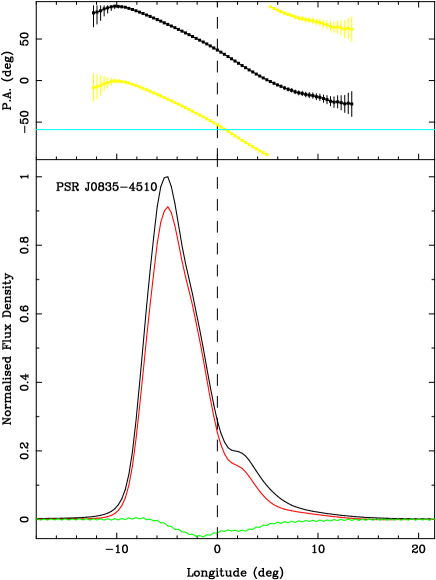
Figure 2: Polarization profile of the Vela pulsar at 1.4 GHz. The bottom panel shows the total intensity (black, thick line), linear polarization (grey line) and circular polarization (pale grey, thin line). The top panel shows the position angle of the polarized radiation as a function of pulse longitude. Two curves are shown. The first (dark points) is the measured PA, the second (lighter points) is the measured PA + 90°. The position angle of the velocity vector, PA_v, is shown as a solid, horizontal line. Pulse longitude 0.0 ($\phi_{0}$) is the closest approach of the line of sight to the magnetic pole as determined from the rotating vector model fit. The PA at this longitude is PA₀ from Equation 1. See also Fig. 1 for a depiction of the relevant angles.

There are a number of cases in which the RM differs significantly from previous values, in particular that of the Vela pulsar. In 1977, the RM of the Vela pulsar was found to be 38 rad m^-2 [Hamilton et al. 1977b]. In a later paper, Hamilton et al. (1985) showed that the RM had increased to 46 rad m^-2 and in fact appeared to be linearly increasing since at least 1970. As far as we are aware there are no further RM measurements quoted in the literature. Our measured value of the RM (2004 November) shows it to have a value of 31.4 rad m^-2, significantly different to the older measurements. Clearly, following an RM increase for at least 15 years (from 1970 to 1985), the RM has now significantly decreased and is currently below the 1970 value. At the time where the RM was increasing, the dispersion measure (DM) was decreasing (see Hamilton et al. 1985). We are not aware of any further DM measurements for Vela but note that DM values depend strongly on profile alignment between different frequencies and care should be taken when comparing results from different epochs.

In the rest of this section, we present polarisation measurements of the individual sources and describe the determination of PA₀, the intrinsic position angle of polarization at $\phi_{0}$, the longitude of closest approach of the line-of-sight to the magnetic pole. Clearly, our choice of $\phi_{0}$ is crucial to our arguments and we justify this choice in detail for each of the pulsars in the paragraphs below. In particular we have taken into account evidence such as profile symmetry, profile frequency evolution and the circular polarization in determining our choice, in a similar fashion to the morphology work of Rankin (1983) and Lyne & Manchester (1988). The final column of table 1 contains the measured value of PA₀ and its error which is derived from the error in the RM determination for each pulsar. Apart from the choice of $\phi_{0}$ itself, additional observational errors due to signal to noise issues contribute only a very small amount. We deal with other sources of error in Section 6.3 below.

Figures 2 and 3 show the polarization profiles for the 25 pulsars in the sample. We first present the results for the Vela pulsar as an illustrative case study, and then the results for the other pulsars in order of increasing Right Ascension.

PSR J0835$-$4510 (Vela; Figure 2): Figure 2 shows the polarization profile of the Vela pulsar from our data. This pulsar represents one of the rare cases where an RVM fit is robust, so we choose $\phi_{0}$ from the fit. The RVM fit constrains both $\alpha$ and $\beta$ reasonably well ($-$137° and 6.5° for these data using the sign conventions in Everett & Weisberg 2001). The fitted location of the closest approach of the line of sight to the magnetic pole is at longitude 0.0 in the figure.

PSR J0525+1115 (Figure 3a): The profile at 1.4 GHz consists of at least three components. The linear polarization is low throughout and the circular polarization changes sign between the first and second component. Following Weisberg et al. (1999), we identify $\phi_{0}$ to be at the longitude of the circular polarization sign change.

PSR J0601$-$0527 (Figure 3b): At this frequency the PA consists of two flat sections, near $-$42° in the leading component and at +75° in the trailing component. We have placed $\phi_{0}$ where the sign of circular polarization changes. At this location there is no linear polarization and hence we cannot measure PA₀. It is possible that $\phi_{0}$ is actually somewhat earlier as the leading component is much more prominent in low frequency observations [Gould & Lyne 1998]. Furthermore, at low frequencies there does appear to be a swing of PA which connects the two flat regions although this is complicated by an orthogonal jump. Absolute PA determination at a lower frequency may resolve this issue.

PSR J0630$-$2834 (Figure 3c): The profile is rather symmetric in this pulsar and we have placed $\phi_{0}$ at the centre of symmetry. There is also rather little evolution of the pulse shape with frequency and it seems likely that the entire emission originates from a component near $\phi_{0}$.

PSR J0742$-$2822 (Figure 3d): As in the case of the Vela pulsar, the PA swing of this pulsar permits a robust RVM fit to be obtained and we used the fitted value of $\phi_{0}$ to locate the closest approach to the magnetic pole. This longitude is also the location of the mid-point of the profile at the 10 per cent emission level.

PSR J0820$-$1350 (Figure 3e): The pulsar shows rather little profile evolution with frequency and also shows a steep swing of polarization through the middle of the pulse. We have therefore located $\phi_{0}$ at the symmetry centre of the profile. An RVM fit can be attempted for this pulsar; although the fit is not very good, the fitted $\phi_{0}$ is coincident with our chosen $\phi_{0}$.

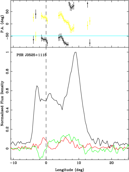
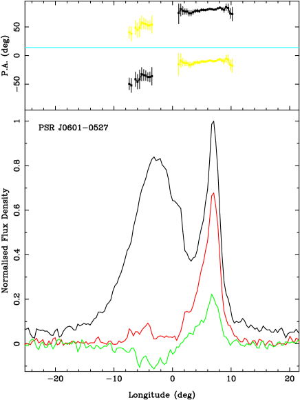
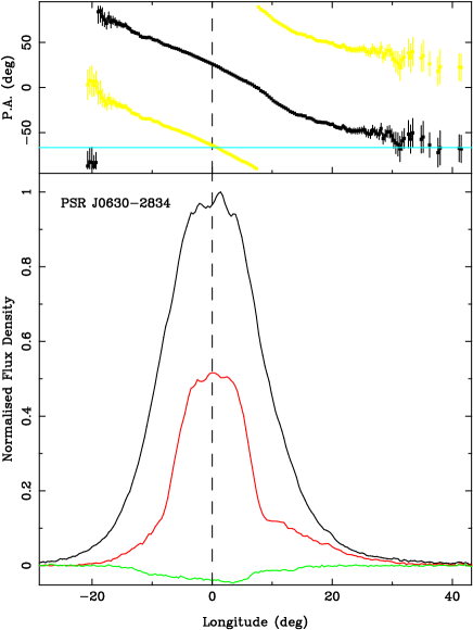
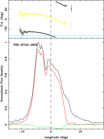
Figure 3: (a)-(d). Polarization profiles at 1.4 GHz for PSR J0525+1115 (top left), PSR J0601$-$0527 (top right), PSR J0630$-$2834 (bottom left) and PSR J0742$-$2822 (bottom right). See caption for Fig. 2 and text for details. The choice of longitude zero for each pulsar is given in the text and is marked with a dashed line where an accurate determination can be made.

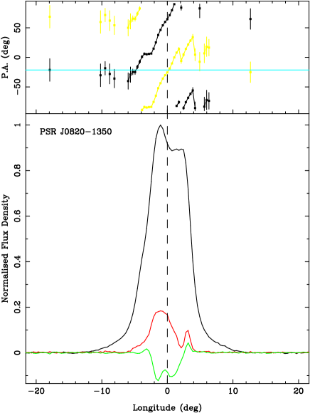
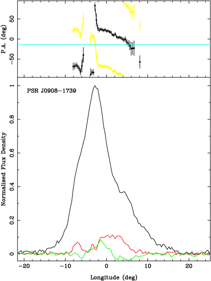
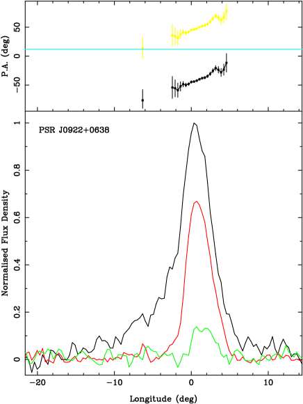
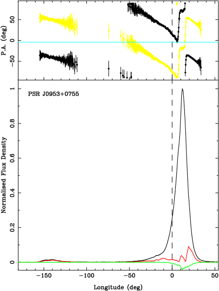
Figure 3: (e)-(h). Polarization profiles at 1.4 GHz for PSR J0820$-$1350 (top left), PSR J0908$-$1739 (top right), PSR J0922+0638 (bottom left) and PSR J0953+0755 (bottom right). See caption for Fig. 2 and text for details. The choice of longitude zero for each pulsar is given in the text and is marked with a dashed line where an accurate determination can be made.

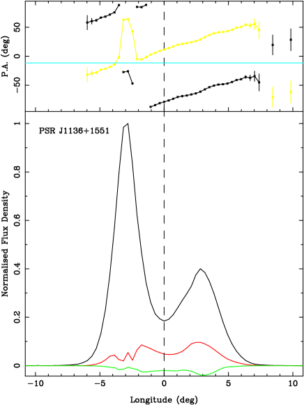
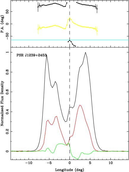
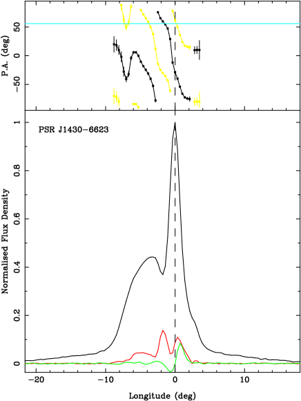
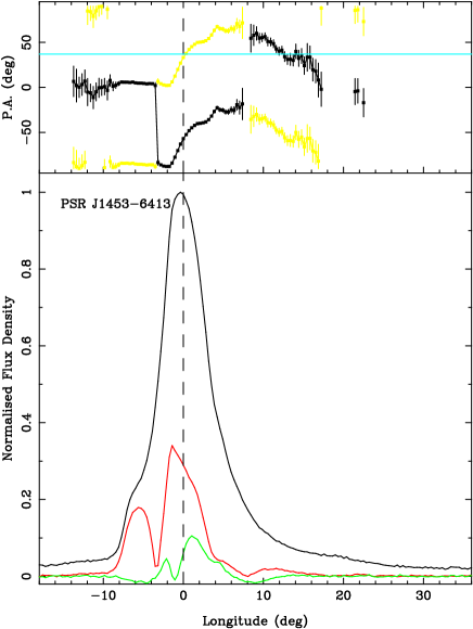
Figure 3: (i)-(l). Polarization profiles at 1.4 GHz for PSR J1136+1551 (top left), PSR J1239+2453 (top right), PSR J1430$-$6623 (bottom left) and PSR J1453$-$6413 (bottom right). See caption for Fig. 2 and text for details. The choice of longitude zero for each pulsar is given in the text and is marked with a dashed line where an accurate determination can be made.

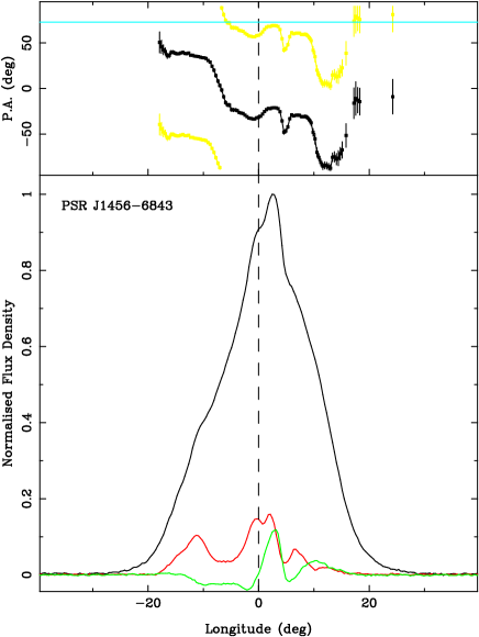
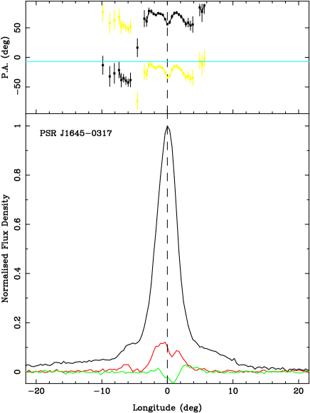
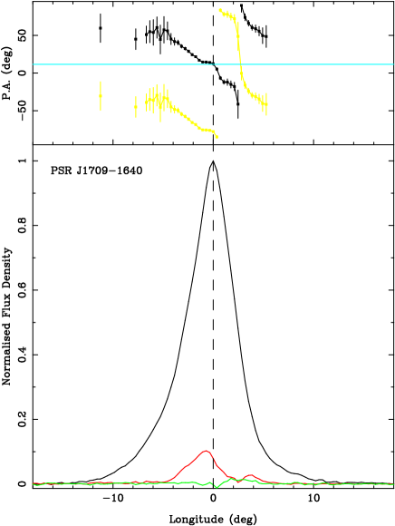
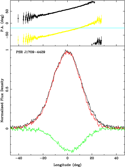
Figure 3: (m)-(p). Polarization profiles at 1.4 GHz for PSR J1456$-$6843 (top left), PSR J1645$-$0317 (top right), PSR J1709$-$1640 (bottom left) and PSR J1709$-$4429 (bottom right). See caption for Fig. 2 and text for details. The choice of longitude zero for each pulsar is given in the text and is marked with a dashed line where an accurate determination can be made.

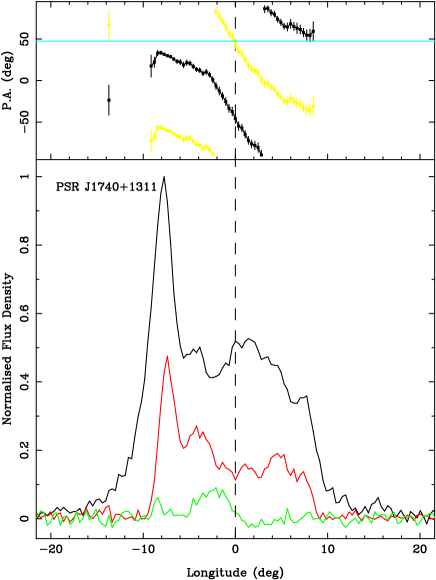
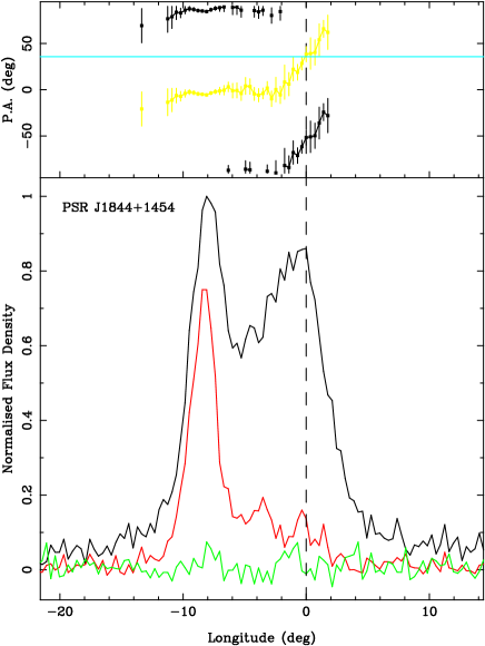
Figure 3: (q)-(t). Polarization profiles at 1.4 GHz for PSR J1740+1311 (top left), PSR J1844+1454 (top right), PSR J1900$-$2600 (bottom left) and PSR J1913$-$0440 (bottom right). See caption for Fig. 2 and text for details. The choice of longitude zero for each pulsar is given in the text and is marked with a dashed line where an accurate determination can be made.

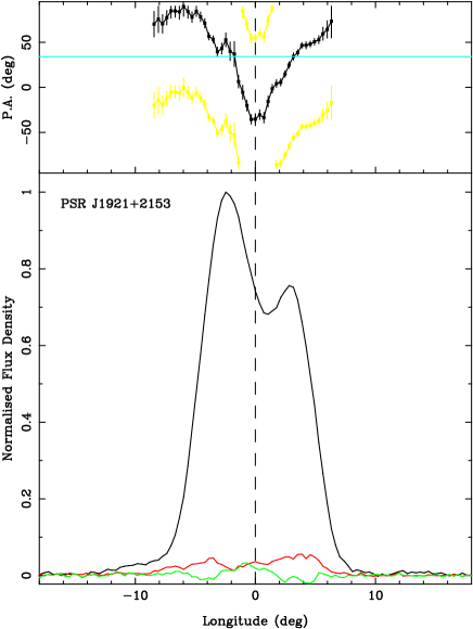
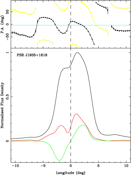
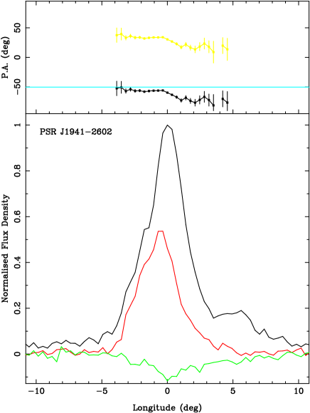
Figure 3: (u)-(x). Polarization profiles at 1.4 GHz for PSR J1921+2153 (top left), PSR J1932+1059 (top right), PSR J1935+1616 (bottom left) and PSR J1941$-$2602 (bottom right). See caption for Fig. 2 and text for details. The choice of longitude zero for each pulsar is given in the text and is marked with a dashed line where an accurate determination can be made.

PSR J0908$-$1739 (Figure 3f): This pulsar is classified as a partial cone (likely the leading edge) by Lyne & Manchester (1988). There is virtually no frequency evolution of the profile between 0.4 and 3.1 GHz lending support to this idea. In Figure 3f we have simply labelled the profile midpoint as longitude zero, although its location is likely to be at significantly later longitudes. We do not assign $phi_{0}$ or $PA_{0}$ for this pulsar.

PSR J0922+0638 (Figure 3g): This pulsar is classified as a partial cone (likely the trailing part) by Lyne & Manchester (1988). Weisberg et al. (1999) provide a comprehensive review of the many observations of this pulsar. It is likely that $\phi_{0}$ is located somewhat earlier than the centre of emission, where the polarized emission is too low to determine PA₀.

PSR J0953+0755 (Figure 3h): The profile consists of a main and interpulse and has (polarized) emission over virtually the whole 360° of longitude. RVM fitting has been attempted by a number of authors as summarised in Everett & Weisberg (2001). The fit given by those authors shows a preference for a single-pole interpretation of the polarization PA swing in this pulsar, unlike other authors who prefer an orthogonal rotator (e.g. Blaskiewicz, Cordes & Wasserman 1991). As Everett & Weisberg (2001) appear to have the best data, we have used their fit to establish the location of $\phi_{0}$ at a longitude which leads the peak of the main pulse by 12°.

PSR J1136+1551 (Figure 3i): The pulsar appears to have a classic double-cone profile and we locate $\phi_{0}$ at the midpoint of the profile.

PSR J1239+2453 (Figure 3j): This pulsar is a classic five-component pulsar. It is likely that the core component is located close to the centre of the profile flanked by the inner and outer cones. This interpretation is backed up by the fact that at high frequencies the core component is less prominent and the swing of the handedness of circular polarization coincides with $\phi_{0}$. The PA swing in this pulsar does not conform to the RVM so no value of $\phi_{0}$ can be obtained from an RVM fit.

PSR J1430$-$6626 (Figure 3k): This pulsar has an extremely complex PA curve at 1.4 GHz and appears to swing through 270°, not allowed in the RVM model. There is rather little profile evolution between 0.4 and 1.4 GHz but the 3.1 GHz observations show a strong decline in the flux density of the leading component. At the peak of the trailing component, the sign of circular polarization changes from negative to positive. It seems likely that $\phi_{0}$ is close to the peak of this component, so we have used this location to estimate PA₀.

PSR J1453$-$6413 (Figure 3l): The profile of this pulsar evolves strongly with frequency. At high frequencies, the component leading the main peak dominates the profile and therefore seems likely to be a conal component. The prominent peak at 1.4 GHz is likely to be the core component and this component also shows a steep swing of PA. We therefore assign $\phi_{0}$ to the peak of this component which also corresponds to a local inflexion point in the PA swing, although a formal fit to the RVM is not possible.

PSR J1456$-$6843 (Figure 3m): Although there appear to be multiple components in the profile of this pulsar there is rather little evolution with frequency across a wide frequency range. The PA swing appears to be simpler at lower frequencies [Hamilton et al. 1977a], although this may be an artifact of low time resolution. We have placed $\phi_{0}$ where the sign of circular polarization changes; this is almost the centre of symmetry of the profile.

PSR 1645$-$0317 (Figure 3n): The pulsar is classified as a core single at low frequencies as it shows a simple single-component profile [Hamilton et al. 1977a]. At 5 GHz and above, the conal outriders become very prominent [von Hoensbroech & Xilouris 1997] and we are therefore confident that the peak of the profile marks $\phi_{0}$.

PSR J1709$-$1640 (Figure 3o): This pulsar is classified as a core single. We locate $\phi_{0}$ at the peak of the profile, which is also the location at which the circular polarization changes sign. We were unable to estimate a value for the RM for this pulsar with sufficient accuracy to improve on the previously listed value.

PSR J1709$-$4429 (Figure 3p): Unfortunately, polarization observations of this pulsar are not particularly illuminating as it is difficult to tell whether $\phi_{0}$ is located near to the single, rather broad component or whether it is instead far out in the pulsar beam (as claimed by Manchester 1996 and Crawford et al. 2001). We therefore do no assign $\phi_{0}$ or PA₀ for this pulsar.

PSR J1740+1311 (Figure 3q): We did not obtain high frequency observations of this pulsar and used the value of RM given in Weisberg et al. (2004). This pulsar is a 5-component pulsar with the core located close to the centre of the profile (see the discussion in Weisberg et al. 2004) and we assign $\phi_{0}$ to this location. The PA swing also shows an inflection point at this same longitude, further strengthening the case that this location marks the magnetic pole crossing.

PSR J1844+1454 (Figure 3r): This pulsar only has a single component at low frequencies. At higher frequencies a conal outrider becomes prominent and dominates the profile above 1.4 GHz. We have located $\phi_{0}$ at the centre of the strong low frequency component.

PSR J1900$-$2600 (Figure 3s): The profile is complex and shows multiple components. The circular polarization shows a characteristic swing with a change of handedness near the centre of symmetry of the profile. This fact, coupled with observations at lower frequencies [McCulloch et al. 1978] make it likely that $\phi_{0}$ is near the centre of the profile.

PSR J1913$-$0440 (Figure 3t): The profile consists of three components at 1.4 GHz. At lower frequencies the trailing component dominates the profile [Hamilton et al. 1977a], whereas at higher frequencies the leading two components become more dominant. Given that there is also a steep swing of PA associated with the trailing component we locate $\phi_{0}$ near the peak of this component.

PSR J1921+2153 (Figure 3u): Weisberg et al. (1999) describe observations of this pulsar made at various frequencies. The pulsar is likely a conal double with $\phi_{0}$ near the profile centre. The PA profile deviates strongly from that expected in the RVM model.

PSR J1932+1059 (Figure 3v): This pulsar has emission over a large longitude range and also has a low-amplitude interpulse; in the figure we show only the main pulse. For a more sensitive observation at this frequency see Weisberg et al. (1999). Many authors have attempted an RVM fit for this pulsar, and these are discussed by Everett & Weisberg (2001). We use their fitted results to locate $\phi_{0}$.

PSR J1935+1616 (Figure 3w): This pulsar is classified as a core single at low frequencies. At high frequencies, conal outriders appear but the central part of the profile remains constant (see the discussion in Weisberg et al. 1999). The PA is rather complicated with a number of orthogonal jumps across the profile and an RVM fit is not possible. We therefore take the location where the circular polarization changes hand to be $\phi_{0}$.

PSR J1941$-$2602 (Figure 3x): The profile of this pulsar also seems likely to be a partial cone. The PA variation is rather flat and there is virtually no profile evolution over a wide frequency range. In particular, the shoulder seen at the trailing edge of the profile remains constant with frequency. We cannot assign $\phi_{0}$ or PA₀ for this pulsar.

6 Discussion

Table 2: PA_v, PA₀ and their offset, $|\Psi|$, for our sample of 25 pulsars. The figure in brackets gives the error in the last digit(s).

Jname	Bname	PAv	PA0	$|\Psi|$	Fig
		(deg)	(deg)	(deg)
Pulsars with $|\Psi|<$10° or $|\Psi|>$80°
J0630$-$2834	B0628$-$28	294(3)	26(2)	88(4)	3c
J0742$-$2822	B0740$-$28	278(5)	$-$81.7(1)	0(5)	3d
J0820$-$1350	B0818$-$13	159(6)	65(2)	86(6)	3e
J0835$-$4510	B0833$-$45	301.0(1)	36.8(1)	84.2(2)	2
J1239+2453	B1237+25	295.0(1)	$-$66(1)	1(1)	3j
J1430$-$6623	B1426$-$66	236(9)	$-$28.5(7)	85(9)	3k
J1453$-$6413	B1449$-$64	217(3)	$-$56.9(4)	86(3)	3l
J1709$-$1640	B1706$-$16	192(16)	15(2)	3(16)	3o
J1740+1311	B1737+13	227(6)	$-$46(4)	87(7)	3q
J1844+1454	B1842+14	36(15)	$-$52(2)	88(15)	3r
Pulsars with 10°$<|\Psi|<$ 80°
J0525+1115	B0523+11	132(16)	$-$65(4)	17(16)	3a
J0953+0755	B0950+08	355.9(2)	14.9(1)	19.0(2)	3h
J1136+1551	B1133+16	348.6(1)	$-$78(2)	67(2)	3i
J1456$-$6843	B1451$-$68	252.7(6)	$-$31.6(6)	76(1)	3m
J1645$-$0317	B1642$-$03	353(3)	56(4)	63(5)	3n
J1900$-$2600	B1857$-$26	202.8(7)	$-$43(2)	66(2)	3s
J1913$-$0440	B1911$-$04	166(11)	$-$68(2)	54(11)	3t
J1921+2153	B1919+21	34(12)	$-$35(2)	69(12)	3u
J1932+1059	B1929+10	65.2(2)	$-$11.3(1)	76.5(2)	3v
J1935+1616	B1933+16	176(1)	10.1(7)	14(1)	3w
Pulsars for which PA0 and hence $\Psi$ cannot be determined
J0601$-$0527	B0559$-$05	194(16)			3b
J0908$-$1739	B0906$-$17	167(2)			3f
J0922+0638	B0919+06	12.0(1)			3g
J1709$-$4429	B1706$-$44	160(10)			3p
J1941$-$2602	B1937$-$26	130(17)			3x

Figure 4: Histograms of observed (top) and simulated (bottom) values of $|\Psi|$. The left hand panels ignore the possibility of orthogonal mode emission so that PA₀=PA_r. The right hand panels include this possibility which then reduces the maximum offset to 45°. Also included is measurement uncertainties in the data with typical value of 10°. Top panels: Observed values of $|\Psi|$ in bins of 10° for 20 pulsars. Bottom panels: Simulated histogram for PA_r parallel to PA_v (thick line), uncorrelated PA_r and PA_v (dashed line) and PA_r perpendicular to PA_v (dot-dash line).

In Table 2 we summarise our results. Columns 3 and 4 show the position angles of the velocity vector, PA_v, and of the linear polarisation, PA₀, at $\phi_{0}$, the closest approach of the line-of-sight to the magnetic pole (see Equation 1), taken from Table 1. Column 5 shows the offset, $|\Psi|$, between PA_v and PA₀ where $\Psi$ is defined as

$$\Psi={\rm PA}_{v}-{\rm PA}_{0};\,\,\,\,\,-90\degr\leq\Psi\leq 90\degr$$ (3)

We force $\Psi$ to lie between $-$90° and 90°by rotating PA₀ by $\pm$180° as necessary (note that any polarized PA has by nature a 180° ambiguity). The error in $\Psi$ comes from a quadrature sum of the errors in PA_v and PA₀.

The table is subdivided into three sections. The top section lists those pulsars for which we find a good relationship between PA₀ and PA_v defined as where $|\Psi|$ is less than 10° or greater than 80°. There are 10 pulsars in this category. The second section lists the 10 pulsars for which there is no clear relation between PA₀ and PA_v i.e. where $|\Psi|$ lies between 10 and 80°. Section 3 lists the 5 pulsars where we can not make a judgement either because there is either no emission at $\phi_{0}$ or the PA swing is too complicated to determine PA₀.

6.1 Statistics

The top left panel of Figure 4 shows the observed distribution of $|\Psi|$ as a histogram for the 20 pulsars for which we have measured $|\Psi|$. If we assume that PA_v and PA₀ are unrelated then the expectation is that the offsets between them should be randomly distributed in the range 0° to 90°. This is shown by the dashed line on the bottom left panel of Fig. 4. The probability of having 7 objects in the top bin, as observed, is very small, $2.6\times 10^{-4}$. A Kolmogorov-Smirnov (KS) test rules out a random distribution at the 94 per cent confidence level. Clearly our measurements show that PA_v and PA₀ must be related in some fashion. Consider now some possible types of relationship between the observables PA_v and PA₀; namely that they are either parallel or perpendicular. To start, we ignore the confounding factor of the orthogonal emission so that PA₀=PA_r (see Fig. 1).

The case where PA_v is parallel to PA_r is a simple one - all the pulsars should fall in the first bin of the histogram. However, measurement errors will broaden this distribution as shown by the solid line on the bottom left panel of Fig. 4. This also does not represent the data; the KS test rules out that these distributions are the same at greater than the 99.9 per cent confidence limit.

The case where PA_v is perpendicular to PA_r is slightly more complex. In this case, the projection effects from the true 3-D vector to the 2-D sky vector will cause the (observed) offset between PA_v and PA₀ to spread away from 90°. This is shown by the dash-dot line on the bottom left panel of Fig. 4 The result looks remarkably similar to the real data apart from the excess in the first two bins. The KS test here does not rule out the possibility that the distributions are the same.

However, the statistics do not take into account the possible presence of orthogonal mode emission which complicates the underlying relationship between PA_r and PA₀, as shown in Fig. 1. Either PA_r is parallel to PA₀ if the pulsar is emitting in the ‘normal’ mode or PA_r is perpendicular to PA₀ if the pulsar emission is in the ‘orthogonal mode’. Simultaneously allowing for either possibility serves to reduce the maximum offset between PA₀ and PA_v to only 45°. The right hand panel of Fig. 4 shows the data and the simulations for such a scenario. The observed histogram appears somewhat broader than the simulation but this may be caused by the possible sources of contamination discussed below. In any case, the results show that we can confidently rule out that PA_r and PA_v are unrelated (dashed line) at the 98 per cent confidence limit. The KS test also rules out the case where PA_r is perpendicular to PA_v (dash-dot line) at greater than the 99 per cent confidence limit but does not rule out that the case where PA_r is parallel to PA_v (solid line) is the same as the observed distribution.

6.2 Information from outside the radio-band

In the previous section we have demonstrated that our radio observations provide clear evidence for a relationship between the spin and velocity vectors of pulsars. The remaining uncertainty as to whether parallel and orthogonal vectors occur or whether the orthogonal PA values are caused by orthogonal emission modes, can be decided by using information obtained outside the radio window. We consider these additional pieces of information in turn.

6.2.1 The Vela pulsar

In Section 1 we noted that, in the Vela pulsar, the axis of the X-ray torus (and hence the pulsar’s rotation axis) had a position angle on the sky of 130° and 310° and that this compared well with the proper motion position angle of 301°. In order to compare this with the polarization position angle, Helfand et al. (2001) used the results of Hamilton et al. (1977) who measured the polarization PA at the peak of the total intensity and obtained an angle of 64° (or 244°). This angle is about 60° different from the position angle of the torus and proper motion. Helfand et al. (2001) then make the bold assertion that as the angle is “almost” 90°, the emission from Vela must be predominantly in a mode polarized orthogonally to the magnetic field lines. Radhakrishnan & Deshpande (2001) discussed the implications of the Vela pulsar’s orthogonal mode emission in the context of the physical model of Luo & Melrose (1995).

There are two issues here. First, 60° is not that close to 90°. Secondly, the peak emission of the profile almost certainly does not coincide with $\phi_{0}$. As described above, this is best measured at the point of greatest swing of the PA curve which, in the Vela pulsar, occurs significantly later than the pulse peak. In our data, the PA at this location appears to be almost exactly 90° offset from PA_v. This provides the observational evidence that the hypothesis by Helfand et al. (2001) and Radhakrishnan & Deshpande (2001) is correct and it is likely that the emission in Vela is perpendicular to the magnetic field direction and that PA_v and the rotation axis are in fact aligned.

6.2.2 The Crab pulsar

Two pieces of evidence from the Crab pulsar also point in this direction. The Crab has PA_v of 292° [Caraveo & Mignani 1999], and interpretation of the X-ray torus indicates that PA_r in the Crab is 124° or 304° [Ng & Romani 2004] meaning that PA_r is parallel to PA_v within the measurement uncertainties.

Secondly, while the radio polarization of this pulsar is very complex, polarization measurements in the optical and UV show a much simpler picture. The main and inter pulses show PA variations which are consistent with a RVM and both have a PA₀ near 124°[Smith et al. 1988, Graham-Smith et al. 1996], very similar to the PA of the X-ray torus. In the radio, at low frequencies the PA of the main and interpulses is 120°, whereas at higher frequencies the PA of the interpulse is 30° [Moffett & Hankins 1999]. Although it is unclear where the main and interpulse emission actually arises (there are competing models for polar cap and light cylinder emission), it is interesting that the polarization PAs match both PA_v and PA_r.

6.2.3 Other pulsars

PSR B0656+14 has PA_v of 93° [Brisken et al. 2003b], and recent optical polarization measurements by Kern et al. (2003) match well with the RVM fit of Everett & Weisberg (2001) allowing a determination of PA₀ of 98°. As we do not have to worry about orthogonal mode emission at optical wavelengths, then PA_r is parallel to PA_v. For the young pulsar PSR B0540$-$69 in the Large Magellanic Cloud, Serafimovich et al. (2004) have shown (weak) evidence that the velocity vector and the jet (and hence rotation axis) align. Finally, other pulsars in the sample of Ng & Romani (2004), PSRs J0538+2817, B1951+32 and B1706–44 also show evidence of tori which also indicate that PA_r is parallel to PA_v.

6.3 Possible contaminants

We are aware of a number of effects that may influence the observed PA_v and PA₀ values, and which may serve to broaden the observed distribution of $\Psi$. Apart from measurement uncertainties and orthogonal mode emission already discussed, we can identify four possible sources of contamination. These are (i) propagation of the radiation through the pulsar magnetosphere, (ii) the effects of differential galactic rotation, (iii) the effects of the galactic potential on the pulsar’s peculiar motion and (iv) the motion of the pre-supernova progenitor star. We will deal with each of these in turn.

6.3.1 Magnetospheric propagation

Blaskiewicz et al. (1991) considered the effects of retardation and aberration of radiation travelling through the pulsar magnetosphere. In brief their argument implies that the position angle sweep lags the profile by an amount which depends on the altitude at which the emission is radiated. A consequence of this is that if $\phi_{0}$ is determined from the RVM fit, it should lag the $\phi_{0}$ determined from the profile characteristics. Furthermore, under the paradigm that different frequencies are emitted from different heights in the magnetosphere the effect should be frequency dependent. We have estimated the size of the effect by computing an emission height at our observing frequency using the prescription in Kijak & Gil (2003) and then deriving the lag between the PA curve and the intensity profile. We find that in the majority of cases this effect is less than 3°, but for the Vela pulsar and PSR J0742$-$2822 the lag is 13.5 and 8.5° respectively. As we have demonstrated, other pieces of evidence suggest that for Vela our determination of $\phi_{0}$ is correct and, in any case, for Vela we have directly measured $\phi_{0}$ from the RVM and hence it does not depend on the aberration value. For PSR J0742$-$2822, Karastergiou & Johnston (2005) have shown that the lag must be significantly smaller than that given in Kijak & Gil (2003). As the derivation of the emission heights of pulsars is highly model dependent we have not included these values in our error budget.

6.3.2 Differential galactic rotation

The proper motion vector of the pulsar at birth is what we really want to compare with PA_r, since the latter quantity will remain fixed in the absence of further torques. Prior to birth, the pulsar’s progenitor star was orbiting the Galactic Centre with a velocity which is location dependent. The difference between this velocity and the orbital velocity at the Sun’s location is the differential galactic rotation component. The measurement of the proper motion is made with respect to the solar system barycentre and therefore includes the effects of differential galactic rotation on the measured value. Since birth, the pulsar has moved in the Galactic potential which has therefore changed its velocity and proper motion vector. In order to determine the rotation of the proper motion vector over the pulsar’s lifetime, it is necessary to integrate equations of motion in the Galactic potential, using as boundary conditions the pulsar’s age, distance, and three-dimensional velocity. The pulsar’s characteristic age, $\tau_{c}$, listed in Table 1 gives a useful indication of the true age but may be in error by a factor of 2 and possibly significantly more for young pulsars [e.g. in Vela [Lyne et al. 1996] and PSR J0538+2817 [Kramer et al. 2003]]. The pulsar distance can be determined from the parallax (where known) or by converting the dispersion measure using the model of Cordes & Lazio (2005) which has an uncertainty for any given object of up to 50 per cent. The observed proper motion gives two components of the velocity, but the radial component is completely unknown although one can justify that it must lie in the range $\pm$1000 kms^-1. A possible handle on the radial velocity can be obtained in the following way. If we assume that the pulsar was born in the Galactic plane and we know its current location and age today, we can adjust the radial velocity so that extrapolating backwards in time forces a birth place in the Galactic plane. Such a technique has been used relatively successfully in the case of the relativistic binary pulsars [Wex, Kalogera & Kramer 2000, Willems, Kalogera & Henninger 2004]. However, given the large uncertainties in the age and distance to the pulsars, we do not feel this approach is appropriate here.

Estimating the differential galactic rotation effect on PA_v at birth is therefore difficult as we do not know the pulsar’s birth location. We can make some general statements, however, using the potential model of Kuijken & Gilmore (1989) which yields a rotation speed of the Sun of 221.4 kms^-1. For young pulsars, born within $\sim$1.5 kpc of the Sun, the differential galactic rotation contributes no more than 10-20 kms^-1 to the overall velocity. We have simulated this effect on our sample and find that it will contribute no more than 5° to the error budget except for very slow moving pulsars. For the most distant pulsar in our sample, PSR J1935+1616 (for which $\Psi$=14°), at a distance in excess of $\sim$5 kpc, the effect could contribute as much as 20°to the error bar. It is therefore important to ensure that the sample contains young, nearby pulsars to minimise this effect.

6.3.3 Acceleration in the galactic gravitational potential

The effect of the galactic potential on the pulsar’s peculiar motion depends critically on the unknown radial velocity. Again, we can make only general statements about the magnitude of this effect. For pulsars born in the vicinity of the Sun, and moving with a velocity of $\sim$300 kms^-1, the time-scale for the proper motion vector to have significantly changed is 15 Myr. We note that 4 of the 5 pulsars with characteristic ages of 3 Myr or less have either $|\Psi|<$10° or $|\Psi|>$80°. Conversely, of the 6 pulsars with ages greater than 10 Myr, only one (PSR J1239+2453) has close match between PA₀ and PA_v. For the 9 remaining pulsars, with intermediate ages, 5 show a correlation between PA₀ and PA_v.

6.3.4 Motion of the progenitor star

Finally, an important effect can occur when the pre-supernova star already has a peculiar velocity. Many high-mass stars are in binary pairs often with short orbital periods. The pre-supernova star can therefore already have a velocity of $\sim$100 kms^-1 or more. If the imparted kick velocity is also only of this order, then the resultant velocity vector will not align with the rotation axis. This scenario was already discussed by Deshpande et al. (1999) who considered it a major reason for their apparent lack of correlation.

6.4 Summary

In summary, we have shown that the case for an alignment of the velocity and spin vectors is very strong. The case is strengthened by the fact that the youngest pulsars in the sample, which suffer from the smallest unknown errors, show the best alignment. In addition, we know that in the case of Vela, the observed emission is in an orthogonal mode. We think it likely therefore that PA_v and PA_r are parallel in all cases but that many (though not all) pulsars emit predominantly in the orthogonal mode. This fits with the values returned from the KS tests on the histrograms in Fig 4 as discussed in section 6.1.

7 Implications

We see no compelling reason to revive the old rocket model of Tademaru & Harrison (1975) even though that model predicts that PA_v should be parallel to PA_r. The problems with that model still remain; it requires pulsar spins of 1 ms at birth, it has difficulty explaining the binary neutron star systems, and polarization data do not favour off-centred dipoles.

In the context of the Spruit & Phinney (1998) model the parallel and orthogonal cases arise in very different ways. In the perpendicular case, the number of impulses must be small and of short duration. In the parallel case, the impulses must be of long duration and can be significant in number. In principle, the two cases lead to different observables. In the perpendicular case the (initial) spin period and velocity should be correlated. In the parallel case, short period pulsars should have a lower mean velocity. In practise, however, distinguishing these cases observationally is difficult, although we note that there is some evidence that short period pulsars are slow moving. Theoretical arguments based on neutrino scattering and parity violation tend to favour long duration kicks but this might only be applicable in magnetic fields greater than 10¹⁵ G [Arras & Lai 1999], values which seem unlikely for the radio pulsars discussed here. More recently, Schmitt, Shovkovy & Wang (2005) have speculated that a neutrino propulsion mechanism associated with the presence of a colour super-conductor in the transverse A phase, produces both high kick velocities and aligned spin and velocity vectors. It is clear that there are theoretical possibilities still to be explored (see also Lai, Chernoff & Cordes 2001).

Both Iben & Tutokov (1996) and Spruit & Phinney (1998) argue that pre-supernova stars do not possess sufficient angular momentum to explain the fast spins of new-born neutron stars. This leads the latter authors to propose their model where one or more off-centre natal kicks is the principal source of young pulsars’ short periods. We wish to point out an important general consequence of such models which seems to have escaped notice, namely that off-centre kick(s) at a radius $r$ that significantly change the magnitude of the pulsar’s spin angular momentum will probably also change the angular momentum direction. This is clear from the vector nature of the equation governing changes in angular momentum, $d\vec{L}/dt=r\times\vec{F}$, where $\vec{F}$ is the force applied. Unless off-centre kick(s) are somehow applied in a fashion that preserves the original rotational symmetry of the star, the angular momentum vector will tip significantly.

Observations of the current parameters of the double neutron star systems allow a determination of the pre-supernova evolution of the system [Wex, Kalogera & Kramer 2000, Willems, Kalogera & Henninger 2004, Thorsett, Dewey & Stairs 2005]. In turn, the kick magnitude and direction imparted to the (second-born) neutron star can be constrained. In PSRs B1913+16, B1534+12 and J0737$-$3039 the kick direction is significantly different from the spin axis of the pre-supernova star and the orbital angular momentum, with the inference that aligned kicks are therefore ruled out. However if, as shown above, the kick imparts both linear and angular momentum to the neutron star, then the spin axis of the newly-born neutron star is not related to either that of its progenitor, or the orbital angular momentum. Consequently, the derived constraints on the kick direction can shed no light on the alignment of spin and velocity vectors.

There is an observational test which can be made. If Spruit & Phinney (1998) are correct, then the misalignment between the spin and orbital angular momenta in the PSR J0737$-$3039 system should be different for the A and B pulsars whereas if the kick only imparts velocity and leaves the pre-supernova spin axis unchanged then the misalignment angles should be identical. These measurements should be possible in the near future. Note that even if the misalignment angles are the same, the spin axes of the two pulsars will not be parallel at the present epoch since their precession rates are different.

8 Conclusions

We have observed 25 pulsars at 1369 MHz, 21 of which were also observed at 3100 MHz. Careful polarization calibration, including accurate RM determination, has enabled us to compute the PA of the polarized radiation at the pulsar to within an accuracy of 2-3°. We have used all available information to deduce $\phi_{0}$, the longitude of the closest approach to the magnetic pole of the star. We then compared the PA of the radiation at this longitude, which is related to the position angle of the axis of rotation, with the velocity vector derived from proper motion measurements.

The combination of precise polarization measurements, accurate RMs and improved velocity information makes this study much more sensitive to any underlying correlation between the spin and velocity vectors. In contrast to previous studies we restricted our sample to young, nearby pulsars where the effects of contaminants discussed earlier have little or no impact.

We find a clear relationship between the velocity vector and the rotation axis. The presence of orthogonal modes in pulsar emission makes it difficult to determine whether the velocity vector is parallel to the rotation axis or perpendicular to it. However, additional information from the optical and X-ray bands for PSR B0656+14, the Crab and Vela pulsars allows us to break this ambiguity: the velocity vector is parallel to the rotation axis and many pulsars emit linear polarisation with PA predominantly perpendicular to the magnetic field lines.

We point out that if the kicks impart both linear and angular momentum to the new-born neutron star, the information about the stellar axis prior to the supernova explosion is lost. Observations of double neutron star systems cannot therefore rule out aligned kicks, contrary to claims in the literature.

References

- [Anderson & Lyne 1983] Anderson B., Lyne A. G., 1983, Nat, 303, 597
- [Arras & Lai 1999] Arras P., Lai D., 1999, ApJ, 519, 745
- [Backer, Rankin & Campbell 1975] Backer D. C., Rankin J. M., Campbell D. B., 1975, ApJ, 197, 481
- [Bailes 1989] Bailes M., 1989, ApJ, 342, 917
- [Bailes et al. 1990a] Bailes M., Manchester R. N., Kesteven M. J., Norris R. P., Reynolds J. E., 1990a, MNRAS, 247, 322
- [Bailes et al. 1990b] Bailes M., Manchester R. N., Kesteven M. J., Norris R. P., Reynolds J. E., 1990b, Nat, 343, 240
- [Blaskiewicz, Cordes & Wasserman 1991] Blaskiewicz M., Cordes J. M., Wasserman I., 1991, ApJ, 370, 643
- [Bock & Gvaramadze 2002] Bock D. C., Gvaramadze V. V., 2002, AA, 394, 533
- [Brisken et al. 2002] Brisken W. F., Benson J. M., Goss W. M., Thorsett S. E., 2002, ApJ, 571, 906
- [Brisken et al. 2003a] Brisken W. F., Fruchter A. S., Goss W. M., Herrnstein R. M., Thorsett S. E., 2003a, AJ, 126, 3090
- [Brisken et al. 2003b] Brisken W. F., Thorsett S. E., Golden A., Goss W. M., 2003b, ApJ, 593, L89
- [Caraveo & Mignani 1999] Caraveo P. A., Mignani R. P., 1999, AA, 344, 366
- [Chatterjee et al. 2001] Chatterjee S., Cordes J. M., Lazio T. J. W., Goss W. M., Fomalont E. B., Benson J. M., 2001, ApJ, 550, 287
- [Cordes & Lazio 2001] Cordes J. M., Lazio T. J. W., 2001, ApJ, Submitted
- [Cowsik 1998] Cowsik R., 1998, AA, 340, L65
- [Crawford, Manchester & Kaspi 2001] Crawford F., Manchester R. N., Kaspi V. M., 2001, AJ, 122, 2001
- [Deshpande, Ramachandran & Radhakrishnan 1999] Deshpande A. A., Ramachandran R., Radhakrishnan V., 1999, AA, 351, 195
- [Dewey & Cordes 1987] Dewey R. J., Cordes J. M., 1987, ApJ, 321, 780
- [Dodson & Golap 2002] Dodson R., Golap K., 2002, MNRAS, 334, L1
- [Dodson et al. 2003] Dodson R., Legge D., Reynolds J. E., McCulloch P. M., 2003, ApJ, 596, 1137
- [Everett & Weisberg 2001] Everett J. E., Weisberg J. M., 2001, ApJ, 553, 341
- [Fomalont et al. 1997] Fomalont E. B., Goss W. M., Manchester R. N., Lyne A. G., 1997, MNRAS, 286, 81
- [Fomalont et al. 1999] Fomalont E. B., Goss W. M., Beasley A. J., Chatterjee S., 1999, AJ, 117, 3025
- [Frail & Scharringhausen 1997] Frail D. A., Scharringhausen B. R., 1997, ApJ, 480, 364
- [Gould & Lyne 1998] Gould D. M., Lyne A. G., 1998, MNRAS, 301, 235
- [Graham-Smith et al. 1996] Graham-Smith F., Dolan J. F., Boyd P. T., Biggs J. D., Lyne A., Percival J., 1996, MNRAS
- [Hamilton & Lyne 1987] Hamilton P. A., Lyne A. G., 1987, MNRAS, 224, 1073
- [Hamilton, Hall & Costa 1985] Hamilton P. A., Hall P. J., Costa M. E., 1985, MNRAS, 214, 5P
- [Hamilton et al. 1977a] Hamilton P. A., McCulloch P. M., Ables J. G., Komesaroff M. M., 1977a, MNRAS, 180, 1
- [Hamilton et al. 1977b] Hamilton P. A., McCulloch P. M., Manchester R. N., Ables J. G., Komesaroff M. M., 1977b, Nat, 265, 224
- [Han, Manchester & Qiao 1999] Han J. L., Manchester R. N., Qiao G. J., 1999, MNRAS, 306, 371
- [Helfand, Gotthelf & Halpern 2001] Helfand D. J., Gotthelf E. V., Halpern J. P., 2001, ApJ, 556, 380
- [Hobbs et al. 2004] Hobbs G., Lyne A. G., Kramer M., Martin C. E., Jordan C., 2004, MNRAS, 353, 1311
- [Hobbs et al. 2005] Hobbs G., Lorimer D. R., Lyne A. G., Kramer M., 2005, MNRAS, 360, 974
- [Hotan, van Straten & Manchester 2004] Hotan A. W., van Straten W., Manchester R. N., 2004, Proc. Astr. Soc. Aust., 21, 302
- [Iben & Tutukov 1996] Iben I., Tutukov A. V., 1996, ApJ, 456, 738
- [Johnston 2002] Johnston S., 2002, Publ. Astron. Soc. Aust., 19, 277
- [Karastergiou & Johnston 2005] Karastergiou A., Johnston S., 2005, MNRAS, In Press
- [Kern et al. 2003] Kern B., Martin C., Mazin B., Halpern J. P., 2003, ApJ, 597, 1049
- [Kijak & Gil 2003] Kijak J., Gil J., 2003, ApJ, 397, 969
- [Kramer 1994] Kramer M., 1994, A&AS, 107, 527
- [Kramer et al. 2003] Kramer M., Lyne A. G., Hobbs G., Löhmer O., Carr P., Jordan C., Wolszczan A., 2003, ApJ, 593, L31
- [Kuijken & Gilmore 1989] Kuijken K., Gilmore G., 1989, MNRAS, 239, 571
- [Lai, Chernoff & Cordes 2001] Lai D., Chernoff D. F., Cordes J. M., 2001, ApJ, 549, 1111
- [Luo & Melrose 1995] Luo Q., Melrose D. M., 1995, ApJ, 452, 346
- [Lyne & Lorimer 1994] Lyne A. G., Lorimer D. R., 1994, Nat, 369, 127
- [Lyne & Manchester 1988] Lyne A. G., Manchester R. N., 1988, MNRAS, 234, 477
- [Lyne et al. 1996] Lyne A. G., Pritchard R. S., Graham-Smith F., Camilo F., 1996, Nat, 381, 497
- [Manchester 1972] Manchester R. N., 1972, ApJ, 172, 43
- [Manchester 1996] Manchester R. N., 1996, in Johnston S., Walker M. A., Bailes M., eds, Pulsars: Problems and Progress, IAU Colloquium 160. Astronomical Society of the Pacific, San Francisco, p. 193
- [Manchester, Taylor & Huguenin 1975] Manchester R. N., Taylor J. H., Huguenin G. R., 1975, ApJ, 196, 83
- [McCulloch et al. 1978] McCulloch P. M., Hamilton P. A., Manchester R. N., Ables J. G., 1978, MNRAS, 183, 645
- [Moffett & Hankins 1999] Moffett D. A., Hankins T. H., 1999, ApJ, 522, 1046
- [Morris, Radhakrishnan & Shukre 1976] Morris D., Radhakrishnan V., Shukre C., 1976, Nat, 260, 124
- [Ng & Romani 2004] Ng C.-Y., Romani R. W., 2004, ApJ, 601, 479
- [Nicastro, Johnston & Koribalski 1996] Nicastro L., Johnston S., Koribalski B., 1996, AA, 306, 49
- [Qiao et al. 1995] Qiao G. J., Manchester R. N., Lyne A. G., Gould D. M., 1995, MNRAS, 274, 572
- [Radhakrishnan & Cooke 1969] Radhakrishnan V., Cooke D. J., 1969, Astrophys. Lett., 3, 225
- [Radhakrishnan & Deshpande 2001] Radhakrishnan V., Deshpande A. A., 2001, AA, 379, 551
- [Radhakrishnan & Rankin 1990] Radhakrishnan V., Rankin J. M., 1990, ApJ, 352, 258
- [Radhakrishnan & Shukre 1986] Radhakrishnan V., Shukre C. S., 1986, Ap&SS, 118, 329
- [Rankin 1983] Rankin J. M., 1983, ApJ, 274, 333
- [Serafimovich et al. 2004] Serafimovich N. I., Shibanov Y. A., Lundqvist P., Sollerman J., 2004, AA, 425, 1041
- [Smith et al. 1988] Smith F. G., Jones D. H. P., Dick J. B., Pike C. D., 1988, MNRAS, 233, 305
- [Spruit & Phinney 1998] Spruit H., Phinney E. S., 1998, Nat, 393, 139
- [Tademaru & Harrison 1975] Tademaru E., Harrison E. R., 1975, Nat, 254, 676
- [Tademaru 1977] Tademaru E., 1977, ApJ, 214, 885
- [Thorsett, Dewey & Stairs 2005] Thorsett S. E., Dewey R. J., Stairs I. H., 2005, ApJ, 619, 1036
- [von Hoensbroech & Xilouris 1997] von Hoensbroech A., Xilouris K. M., 1997, A&AS, 126, 121
- [Weisberg et al. 1999] Weisberg J. M. et al., 1999, ApJS, 121, 171
- [Weisberg et al. 2004] Weisberg J. M., Cordes J. M., Kuan B., Devine K. E., Green J. T., Backer D. C., 2004, ApJS, 150, 317
- [Wex, Kalogera & Kramer 2000] Wex N., Kalogera V., Kramer M., 2000, ApJ, 528, 401
- [Willems, Kalogera & Henninger 2004] Willems B., Kalogera V., Henninger M., 2004, ApJ, 616, 414