Transit flow models for low and high mass protostars

Abstract

In this work, the gas infall and the formation of outflows around low and high mass protostars are investigated. A radial self-similar approach to model the transit of the molecular gas around the central object is employed. We include gravitational and radiative fields to produce heated pressure-driven outflows with magneto-centrifugal acceleration and collimation. Outflow solutions with negligible or vanishing magnetic field are reported. They indicate that thermodynamics is a sufficient engine to generate an outflow. The magnetized solutions show dynamically significant differences in the axial region, precisely where the radial velocity and collimation are the largest. They compare quantitatively well with observations. The influence of the opacity on the transit solutions is also studied. It is found that, when dust is not the dominant coolant, such as in the primordial universe, mass infall rates have substantial larger values in the equatorial region. This suggests that star forming in a dust-free environment should be able to accrete much more mass and become more massive than present day protostars. It is also suggested that molecular outflows may be dominated by the global transit of material around the protostar during the very early stages of star formation, especially in the case of massive or dust-free star formation.

1 Introduction

The understanding of star formation has changed dramatically during the last two decades thanks to the development of both instrumental and numerical techniques. However, while the picture of the main stages of low mass star formation is becoming clearer, the situation for massive objects remains problematic. In the present paper, we address the problem of the origin of outflows and infall around protostars over a wide range of masses.

At present, the stages of low mass protostar evolution are empirically divided in four classes (see for example André et al. (2000) for a review) corresponding to the evolutionary sequence from the initial collapse to a new star. “Class 0” protostars correspond to the earliest stage of star formation. Observationally, they appear deeply embedded in a circumstellar dusty envelope (detected in sub-millimeter wavelengths) that is more massive than the central stellar mass. Furthermore, they show powerful bipolar ejections of material in the form of collimated CO outflows which distinguish them from the pre-stellar phase of star formation (a gravitationally bound core within a molecular cloud).

The next stage of the star formation process corresponds to “Class I” objects which are typically $10^{5}$ year old and are characterized by a positive slope of their spectral energy distributions (SEDs) between 2.2 and 10-25 $\mu$m. They are still surrounded by a diffuse circumstellar envelope but are also surrounded by a disk from which the accretion onto the central object takes place. At this stage, the mass contained in the envelope is smaller than the mass of the central protostar. Like Class 0 objects, they also produce bipolar outflows (optical jets and molecular outflows) but these are less ($\sim$ 1 order of magnitude) powerful than those observed for Class 0 protostars (Bontemps et al., 1996).

Class II and III objects (resp. classical and weak-line T Tauri stars) are the final two stages in evolutionary sequence of protostars. These correspond to pre-main sequence stars surrounded by an accretion disk (optically thick (Classical) or thin depending on the degree of evolution) but which do not have a circumstellar envelope, as opposed to Class 0 or 1 objects.

Formation of massive stars ($M\geq 10M_{\odot}$), is less well understood but two main theories have emerged: i) the coalescence scenario in which massive stars are formed by the merging of intermediate mass objects (Bonnell et al., 1998) and ii) the accretion scenario, originally applied to massive star by Beech & Mitalas (1994), where a massive star forms thanks to large accretion rates ($10^{-4}-10^{-2}\;M_{\odot}$) onto the central object (Norberg & Maeder, 2000; Behrend & Maeder, 2001). The main difficulty of the merging scenario arises when one considers the high stellar densities needed for it to be efficient. On the other hand, it is difficult to accrete gas onto a very luminous star so that the upper mass of the accretion scenario is rapidly reached.

Whatever the mass of the central object is, it appears that the accretion of material is accompanied by strong bipolar outflows. During the last two decades, starting with the first outflow observation from a forming star by Snell et al. (1980), the number of outflow observations has increased to the point that this phenomenon is now widely believed to affect every forming star. Bipolar outflows allow the forming star to transport any excess of angular momentum. They can be classified as either atomic jets or molecular outflows, according to their properties.

Jets are fast ($\sim 100-300$ km s^-1), well-collimated (opening angle $<$ 10^∘), and mostly constituted of atomic material. Many models and simulations attempt to describe how they can be launched from the magnetized accretion disk of the protostar (Ferreira, 1997; Ouyed & Pudritz, 1997), and their magneto-centrifugal origin is commonly accepted. However, the nature of the exact mechanism, be it a disk wind (Blandford & Payne, 1982) or the asymptotic collimation of an $X$-wind (Shu et al., 1995, 2000), is still debated.

Molecular outflows (often traced by CO and H₂ molecules) are more massive, slower ($\sim$ tens of km s^-1) and less collimated than jets. The driving mechanism of these outflows is still open to discussion but the jet-driven bow shock model (Raga & Cabrit, 1993; Chernin et al., 1994; Downes & Ray, 1999; Ostriker et al., 2001) and the wind-driven model (Shu, 1991; Shu et al., 2000) are the two main theories that have emerged. In the jet-driven model, the bow shock surface created at the head of the jet transfers momentum to the ambient medium thus producing a thin shell that is identified as the molecular outflow. In the second approach, a wide-angle wind creates two bipolar wind-blown bubbles that sweep up the ambient material (then referred to as the molecular outflow).

For low and intermediate mass star formation, the morphologies and kinematics of the observed outflows are generally explained by one of these two models: some outflows present jet-driven features (e.g. HH212, Orion S outflow, Rodríguez-Franco et al. (1999)) whereas others (e.g. VLA 0548) show wind-driven signatures (Lee et al., 2000, 2001). However, when massive star formation is considered, the observations cannot be matched by any of these two models (Churchwell, 1997, 2000). The formation of massive stars gives rise to molecular outflows showing different properties than the ones recorded in low and intermediate mass star formation: they are very massive ($\sim$ tens of solar masses and, in some cases, more massive than the central stars that presumably drive them), poorly collimated and also faster than in the case of low mass star formation. According to Churchwell (1997, 2000), jets cannot entrain more than a few solar masses and certainly not the tens of solar masses observed in massive outflows. Furthermore, the wide opening angles observed are hardly explained by the entrainment from a collimated jet. On the other hand, if entrainment by a wide-angle wind allows a large opening angle for the outflow, it cannot match the velocities reached by massive outflows.

In this paper, we present a general radial self-similar model for the flows surrounding young forming stars, applicable in both low and high mass star formation. The paper is laid out as follows: in Sect. 2, we describe the model and its equations and show corresponding hydrodynamical solutions in Sect. 3; some magnetized solutions are then presented, together with a study of the influence of changes in the opacity, in Sect. 4; we give the main properties of the model in Sect. 5 and discuss them in Sect. 6 before concluding.

2 Theoretical basis of Transit Models

The present models are based on ideal MHD with the assumption of radial self-similarity and a simplified treatment of radiation (Fiege & Henriksen, 1996; Lery, 2003).

Spherical coordinates are used: the system is centered on the protostar, the $x-y$ plane corresponds to the equatorial plane and the poloidal angle $\theta$ is taken relative to the rotational axis of the central object.

2.1 Fluid equations

We describe the gas with the usual macroscopic quantities: density $\rho$, velocity ${\rm\bf v}$, pressure $p$ and temperature $T$. The size of the system is such that the conditions for ideal MHD are fulfilled. We further assume steady-state ($\partial/\partial t=0$), axial symmetry around the rotational axis ($\partial/\partial\phi=0$). The standard ideal MHD equations then reduce to:

$$\nabla\cdot(\rho\mathbf{v})=0$$ (1)

$$\frac{1}{\rho}\nabla p+\nabla\Phi+\left(\mathbf{v\cdot\nabla}\right)\mathbf{v}=\frac{1}{4\pi\rho}\nabla\times\mathbf{B}\times\mathbf{B}$$ (2)

$$\nabla\cdot\mathbf{B}=0\;.$$ (3)

The magnetic Reynolds number being much greater than unity, the diffusion term in the induction equation can be neglected, and the magnetic field lines are frozen in the plasma. The induction equation becomes

$${\nabla\times(\mathbf{v}\times\mathbf{B})=0}$$ (4)

which directly implies

$$\mathbf{v}\times\mathbf{B}=\nabla\Psi$$ (5)

where $\Psi$ is the electric potential (${\mathbf{E}=-\nabla\Psi}$). A non-zero toroidal electric field could convect the magnetic poloidal field lines into a sink on the axis of the system. To ensure a zero toroidal electric field, the only requirement from Eq. (5) is $\mathbf{v}_{p}\propto\mathbf{B}_{p}$ (Chan & Henriksen, 1980; Henriksen, 1996), where the subscript $p$ denotes the poloidal component of the field (${\mathbf{v}=\mathbf{v}_{p}+\mathbf{v}_{\phi}}$ and $\mathbf{B}=\mathbf{B}_{p}+\mathbf{B}_{\phi}$).

We also consider the equation of state for ideal gas, i.e. $p=nkT$.

Note also that the purely hydrodynamical problem will be studied by using Eq.(1) and setting the RHS in Eq.(2) to zero.

2.2 Self-similar treatment

2.2.1 Self-similarity - general statements

A phenomenon is called self-similar if the spatial (or temporal) distributions of its properties at various different times (or locations) can be obtained from one another by a similarity transformation. The investigation of the full phenomenon can then be reduced to the study of the properties of the system for only a specific time (or location). If the origin of time can be chosen arbitrarily, the scales of length and mass are also arbitrary, and the system is ‘scale-free’. The system of partial differential equations (PDE) that describe the problem is transformed to a set of ordinary differential equations (ODE), which drastically simplifies the investigation.

Self-similar models turn out not only to describe the behavior of physical systems under some special conditions, but also describe the intermediate-asymptotic behavior of solutions to wider classes of problems in the range where these solutions no longer depend on the details of the initial and/or boundary conditions, yet the system is still far from being in an ultimate equilibrium state (Barenblatt & Zel’dovich, 1972). For an extensive review of self-similarity, the reader is referred to Barenblatt (1996). In present case of star formation, we express each variable using the following self-similar form

$$L(r,\theta)=L_{0}\times\left(\frac{r}{r_{0}}\right)^{\alpha}\times l(\theta).$$ (6)

The constant $L_{0}$ has the dimensions of the variable and is directly dependent on the parameters of the problem such as the mass or the luminosity of the central object. The free parameters are the self-similar indices $\alpha$ and the fiducial scale $r_{0}$.

2.2.2 Self-similar fluid quantities

Several observations of the protostellar environment favor our self-similar approach since they show that radial density profiles in regions of isolated star formation are well represented by a power-law $\rho\propto r^{-p}$ with $p\sim 0.5-2$ (e.g. L1527 has been found to have $p$ in the range of 1.5-2 Ladd et al. (1991)). Indeed, in some cases, density profiles are reproduced by most hydrostatically supported ($p=2$) or free infalling ($p=1.5$) cloud core, e.g. Shu (1977). In some other cases, the slope has been found to be much shallower than the ones predicted by the standard models. Density profiles as shallow as 0.5-0.9 can be interpreted as the presence of a magnetic (Barsony & Chandler, 1993) or rotational support(Chandler et al., 1998) of the core.

We now apply our assumptions to the ideal MHD equations. Dimensional analysis allows us to determine the index of each variable as a function of a single free self-similar parameter, $\alpha$. The systems then reads

$$\rho(r,\theta)=\frac{M}{r_{0}^{3}}\left(\frac{r}{r_{0}}\right)^{2\alpha-\frac{1}{2}}\mu(\theta)$$ (7)

$$p(r,\theta)=\frac{GM^{2}}{r_{0}^{4}}\left(\frac{r}{r_{0}}\right)^{2\alpha-\frac{3}{2}}P(\theta)$$ (8)

$$T(r,\theta)=\frac{\bar{\mu}m_{H}}{k_{B}}\frac{GM}{r_{0}}\left(\frac{r}{r_{0}}\right)^{-1}\Theta(\theta)$$ (9)

$$\mathbf{v}(r,\theta)=\left(\frac{GM}{r_{0}}\right)^{\frac{1}{2}}\left(\frac{r}{r_{0}}\right)^{-\frac{1}{2}}\mathbf{u}(\theta)$$ (10)

$$B_{r,\theta,\phi}(r,\theta)=\left(\frac{GM^{2}}{r_{0}^{4}}\right)^{\frac{1}{2}}\left(\frac{r}{r_{0}}\right)^{\alpha-\frac{3}{4}}\frac{u_{r,\theta,\phi}(\theta)}{y_{p,p,\phi}(\theta)}.$$ (11)

In these expressions, $G$ is the gravitational constant, $k_{B}$ the Boltzmann constant, $m_{H}$ the mass of the proton, $\bar{\mu}$ the mean molecular weight (we use $\bar{\mu}=2$), and $M$ the mass of the central object. The fiducial scale $r_{0}$ is a radius of reference. The self-similar assumption is valid only above this radius (see Sect. 2.3.2). Note also that in Eq. (11), the subscript $p$ stands for “poloidal’. The self-similar index $\alpha$ is a free parameter that lies between $-1/2<\alpha\leq 1/4$. In particular, $\alpha=-1/2$ yields to pure radial accretion. This issue is discussed in Fiege & Henriksen (1996) and the behavior of the solutions with $\alpha$ can be found in Lery et al. (1999). Note that the hydrostatic ($p=-2\alpha+1/2=2$) and the free infalling ($p=1.5$) cases cannot be treated by the present model.

For the remainder of this paper, we choose $\alpha=-0.2$ in most cases. From Eq.(7), we infer $\rho\propto r^{-0.9}$, which corresponds to a shallow density profiles where rotation and magnetic field can drive substantial effects.

In a nearly study on self-similar transit models (Fiege & Henriksen, 1996), the same proportionality relationship between each component of the velocity and magnetic field was taken. All the components of the electric field Eq.(5) were then equal to zero. Such a configuration has the virtue of great simplicity, but does not allow for the existence of a Poynting flux. They obtained fast axial outflows but the luminosities required to drive them were as high as $10^{5}-10^{6}\;L_{\odot}$. In a subsequent work (Lery et al., 1999), this constraint has been relaxed. Only the necessary proportionality condition on the poloidal components of the velocity and magnetic field (${\bf v}_{p}\propto{\bf B}_{p}$) was satisfied and the importance of the Poynting flux taken into account. The corresponding solutions were found to be faster and required a comparatively smaller source luminosity to be driven. In this work, we use the formalism and conditions from Lery et al. (1999) based on Poynting flux driving mechanism ($y_{p}(\theta)\neq y_{\phi}(\theta)$) that breaks the collinearity between ${\bf B}$ and ${\bf v}$.

2.2.3 Self-similar radiation treatment

In the early stages of star formation, most of the luminosity comes from the accretion shock created by the infalling material. Later on, the accretion rate reduces and the radiation is dominated by the protostar luminosity. Here, we use a simplified description for radiation (Fiege & Henriksen, 1996) that allows us to use an analytical self-similar approach.

Radiative diffusion:

The steady-state energy conservation equation, that includes the mechanical and radiative energy fluxes, simply reads

$$\nabla\cdot\left[\rho{\bf v}\left(h+h_{rad}+\frac{v^{2}}{2}+\Phi_{grav}\right)+{\bf F}_{rad}\right]=0$$ (12)

where:

• $h$ is the specific enthalpy: $h=u+p/\rho$, with $u$ the internal specific energy and $p$ and $\rho$ respectively the pressure and density.

• $h_{rad}$ is the specific radiative enthalpy. For an isotropic radiation field, the radiative pressure is $p_{rad}=u_{rad}/3$, with $u_{rad}$ the radiative energy density. Then, $h_{rad}$ is defined as $h_{rad}=(u_{rad}+p_{rad})/\rho=4p_{rad}/\rho$

• $\Phi_{grav}$ is the gravitational potential created by the central protostar.

• ${\bf F}_{rad}$ is the radiative flux.

For the radiation independently, the radiative energy conservation reads (Mihalas & Klein, 1982)

$$\nabla\cdot\left({\bf F}_{rad}+\rho{\bf v}h_{rad}\right)=-\frac{\kappa\rho}{c}{\bf v}\cdot{\bf F}_{rad}$$

where $c$ is the speed of light and $\kappa$ the opacity. It is re-written at the zero-th order in (v/c)

$$\nabla\cdot{\bf F}_{rad}=0\;.$$ (13)

This equation decouples the mechanical energy fluxes from the radiative ones in Eq.(12). Furthermore, when taking the zero-th order in (v/c) in Eq.(12), the $h_{rad}$ term disappears. This means that the radiative pressure is neglected, i.e. the photons transfer no momentum to the gas.

The previous statements are valid for any particular form of the radiative flux ${\bf F}_{rad}$. In this work, we use the radiative diffusion approximation

$$\mathbf{F}_{rad}=-\frac{c}{\kappa\rho}\nabla p_{rad}$$ (14)

where the radiative flux is directly linked to the energy density (then to the radiative pressure). This assumes that the mean free path of a photon is very short compared to the characteristic length of the system. We use the black-body radiative pressure for $p_{rad}$ which, at the temperature $T$ is given by

$$p_{rad}=\frac{4}{3}\frac{\sigma}{c}T^{4}$$ (15)

with $\sigma$ the Stefan-Boltzmann constant.

Opacity:

For the sake of simplicity, we choose an opacity defined by Kramer’s law,

$$\kappa=\kappa_{0}\left(\frac{\rho}{1\rm{~{}g~{}cm}^{-3}}\right)^{a}\left(\frac{T}{1\rm{~{}K}}\right)^{b}\;,$$ (16)

where the values of the exponents $a$ and $b$ are defined according to the type of coolant considered. These parameters will be discussed in greater detail in section 4.3. For example, when the cooling is dust-dominated, $a=0$ and $b=2$ (e.g. Pollack et al. (1985)). The constant $\kappa_{0}$ is determined using a numerical code developed by Semenov et al. (2003) which calculates opacities over a wide range of gas densities and temperatures, given a solar-type metallicity. This code includes different shapes and compositions for the dust particles. In this work, we use the “homogeneous compact spherical dust” configuration to compute the opacity. Moreover, we focus on molecular outflows which temperature range (10-100 K) is in the dust-dominated regime of opacity. In that case, the dust being such an efficient coolant, the opacity is independent of the density of the gas, i.e. $a=0$. The opacities, obtained for a gas density of $10^{-18}$g cm^-3, are plotted in Fig. 1 and can be fitted by a power-law. We found the Kramer’s coefficient of the temperature to be $b=2$ and $\kappa_{0}\sim 2\times 10^{-4}$ cm² g^-1 for the dust dominated regime.

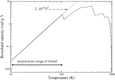
Figure 1: Opacity as a function of temperature computed with the code from Semenov et al. (2003) for a gas density of $10^{-18}$g cm^-3.

Following Eq.(6), the self-similar radiative flux reads

$$\mathbf{F}_{rad}(r,\theta)=\left(\frac{GM}{r_{0}}\right)^{\frac{3}{2}}\frac{M}{r_{0}^{3}}\left(\frac{r}{r_{0}}\right)^{\alpha_{f}-2}\mathbf{f}(\theta)\;.$$ (17)

Using the self-similar expression of the temperature $T$ in Eq. (15) and combining Eq. (14) and (15), one finds $\alpha_{f}$ to be $\alpha_{f}=b-3+2(a+1)(1/4-\alpha)$.

Furthermore, the inclusion of radiative diffusion in the model constrains the expression of the fiducial scale $r_{0}$. Indeed, the RHS and LHS multiplicative constants of the self-similar expansion of Eq. (14) have to be equal: this leads to the following expression of $r_{0}$,

$$r_{0}=\left(\frac{3\kappa_{0}}{4a_{s}c}M^{2+a}\left(GM\right)^{b-\frac{5}{2}}\left(\frac{\bar{\mu}m_{H}}{k_{B}}\right)^{b-4}\right)^{\frac{2}{5+6a+2b}}$$ (18)

where $a_{s}=4\sigma/c$ with $\sigma$ the Stefan-Boltzmann constant.

It is worthwhile to note that when diffusive radiation is discarded, the fiducial scale is not explicitly defined. In that case, the fiducial radius remains a free parameter and a characteristic length has to be chosen on observational or physical criteria (see Lery et al. (1999) and Sect. 2.3.2 for the discussion on this issue).

2.3 Methods

2.3.1 Integration

Assuming self-similarity, the PDE system of HD/MHD equations is transformed into an ODE system where all variables depend only on the poloidal angle $\theta$,

$$\frac{{\rm d}l_{i}(\theta)}{{\rm d}\theta}=A_{ij}\;l_{j}(\theta)\;.$$ (19)

In the MHD (HD) case, eight (six) coupled equations constitute the system. We consider the problem as an initial value problem (IVP) and use the values of the variables ($u_{r},u_{\theta},u_{\phi},\mu,y_{p},y_{\phi},\Theta$ and $f_{\theta}$) as input parameters at a given angle. Note that $y_{p}$ and $y_{\phi}$ are not present in the HD case. In practice, we start the integration close to the rotational axis, typically at $\theta_{0}=10^{-2}$ rad. We provide the initial values near the axis, i.e. a positive $u_{r}$ for the outflow, $u_{\theta}$ negative for the circulation pattern and $u_{\phi}$ chosen to be positive. We look for solutions covering $\theta=\theta_{0}$ to $\theta=\pi/2-\epsilon$ as the polar axis and the equatorial plane are excluded by the self-similar treatment (Fiege & Henriksen, 1996).

2.3.2 Dimensions and the fiducial scale r₀

For each solution, dimensional quantities can be calculated using Eq.(7) to (11) and Eq.(17). From these equations, for any physical quantity, only the mass of the central object $M$ and the fiducial scale $r_{0}$ are required to compute the dimensional quantities at a given radius $R$. Without radiative diffusion, $r_{0}$ remains a free parameter (see Lery et al. (1999) for more details).

In Fig. 2, the fiducial scale (from Eq.(18)) is plotted as a function of the Kramer’s coefficients $a$ and $b$ for a one solar mass protostar and $\kappa_{0}=2\times 10^{-4}$cm² g^-1.

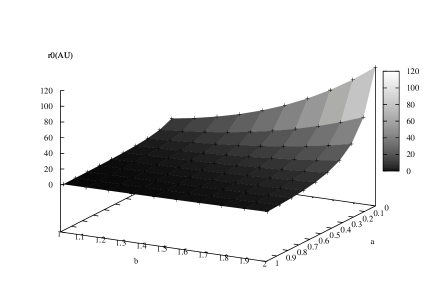
Figure 2: Variation of $r_{0}$ with the Kramer’s opacity parameters. The values are obtained for a one solar mass protostar.

The variation of $r_{0}$ with the Kramer’s parameters is quite stiff and $r_{0}$ quickly drops from $\sim$ 100 AU to 0 as $a$ increases and/or $b$ decreases from the dust-dominated case. Note that $r_{0}$ is a lower limiting radius for the validity of self-similarity.

For physical reasons, $r_{0}$ should also be limited to the region where the hypotheses of the model still apply. For example, close to the protostar, the radiation pressure could have non-negligible dynamical effects preventing the model to be applicable there.

2.3.3 Selection criteria of the solutions

Firstly, we select solutions showing outflowing motions near the axis region and infall near the equatorial plane. This means that radial velocity $u_{r}$ must change sign once for an angle $\theta_{\rm open}$ which is the opening angle of the outflow: for $\theta>\theta_{\rm open}$, $u_{r}$ is negative and trace the infall; for $\theta<\theta_{\rm open}$, $u_{r}$ is positive and the gas is flowing outward.

Secondly, we use the self-similar expressions of the physical quantities to go from the dimensionless variables to the dimensioned ones: we define the mass of the central object (we typically choose 1 $M_{\odot}$), an observational radius ($\sim 5\times 10^{3}$ AU) and a type of coolant (values of $a$ and $b$ in the opacity).

Finally, we discard unphysical solutions, i.e. solutions that do not fit in the range of observations.

3 Hydrodynamical solutions

Pure hydrodynamical (HD) solutions can apply in situations where magnetic fields are either very weak (e.g., primordial universe) or not dynamically dominant for the movement of the gas (early stages of the collapse). Besides, studying a purely HD problem allows us to distinguish the effects of the radiation and density gradients from those of the magnetic field (see Sect. 4).

We find HD solutions with both infall and outflows and they all show common properties: i) the outflow is very narrow and ii) always quite slow ($<10$ km s^-1 for a one solar mass central object) and iii) infall is occurring in the rest of the domain in a quasi-spherical way.

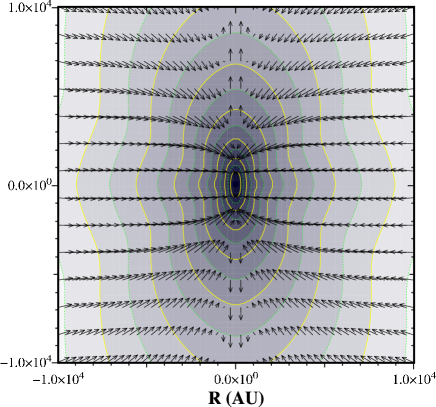
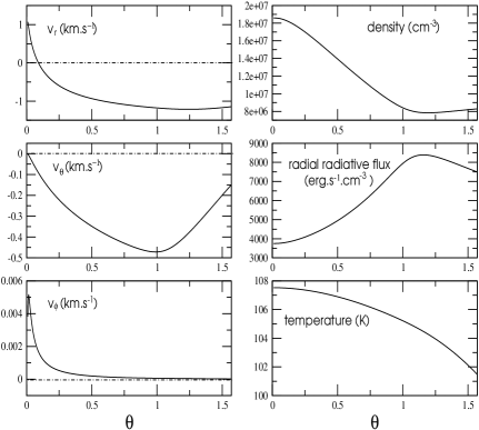
Figure 3: Left panel: a typical solution for the HD case represented in the poloidal plane $(r,\theta)$. The iso-density contours and velocity field are plotted. Right panel: corresponding values of the velocity, density, temperature and radial radiative flux at a distance of 5000 AU from the central protostar, with respect to the poloidal angle $\theta$. For this particular solution, the input values of the dimensionless quantities are: the velocities $u_{r}=2.54$, $u_{\theta}=-4.46\times 10^{-3}$, $u_{\phi}=9.05\times 10^{-3}$, the density $\mu=3.62\times 10^{-3}$, the temperature $\Theta=1.81$ and the $\theta-$component of the radiative flux $f_{\theta}=7.92\times 10^{-1}$.

For illustration, a typical hydrodynamical solution is plotted in Fig. 3: the left panel corresponds to the density contours and velocity field of the solution in the poloidal plane, and the right panel to different quantities plotted (at a fixed distance of 5000 AU) as a function of the poloidal angle $\theta$. The central object was assumed to be a one solar mass protostar. The Kramer’s opacity parameters are those of a dust-dominated opacity (namely, $a=0$ and $b=2$).

The infall-outflowing pattern is traced by the radial velocity: a negative radial velocity corresponds to an infall motion whereas a positive one is the signature of an outflow. Note also that $v_{\theta}$ keeps a constant negative sign, implying that all the material is being redirected outward in this particular solution. This will not be the case for solution with “net infall” (see Sect. 4.2). The $\theta-$velocity characterizes the movement of the gas towards the rotational axis. Here, the maximum reached by $v_{\theta}$ is $\sim$ 0.45 km s^-1: this is a small value that implies a weak “collimation” of the flow. For this solution, the outflow has a velocity of approximatively $\sim$ 1 km s^-1 and a $\sim$ 5^∘ opening angle. The system is also almost non-rotating as $v_{\phi}$ is close to zero over the entire domain. The values of the number density (upper-left panel) are in the order of $10^{6}$ cm^-3 at 5000 AU and shows a increase towards the axis of rotation. However, the density at the axis is only twice as large as the one near the equator, emphasizing a quasi-spherical infall. At a given radius, the temperature (lower right panel) is also almost constant ($\sim$ 100 K at 5000 AU) which characterizes an isothermal infall.

Qualitatively, this solution presents some common features with observations. First we have an outflow. We also find that the fastest material was also the most collimated (Bachiller, 1996; Richer et al., 2000). This is precisely the case here where the positive part of the radial velocity (outflow) that decreases when the angle from the axis increases. However, physical quantities (velocity, temperature and density) do not match with observations. In particular, the density is an order of magnitude too high to fall in the observed density range ($10^{4}-10^{5}$ cm^-3), and also the velocity is too small.

In conclusion, we have shown that our models can produce outflows that can be launched from thermodynamical effects only. We have a simple heated quadrupolar model for infall and outflow. The qualitative characteristics of the hydrodynamical solutions are similar to the observed protostellar outflows but are quantitatively too dense, too slow and too narrow for typical solar mass objects.

4 MHD solutions

Typical molecular outflows of low mass protostars have observed velocities $\sim$ 20 km s^-1 and have a large range of initial opening angles: from $\lesssim$ 30^∘ for class 0 to $\gtrsim$ 90^∘ for class 1 objects (Bachiller, 1996; Bachiller & Tafalla, 1999). Their typical densities lie around $10^{4-5}$ cm^-3. Our hydrodynamical model cannot power such outflows and we now include the magnetic field in the model.

There are two main issues that we wish to address with our magnetized model:

• Class 0 low mass protostars: they show powerful, highly collimated molecular outflows despite their very young age.

• The formation of massive stars: they present very massive outflows (mass loss rates $\sim 5\times 10^{-3}$ $M_{\odot}$ yr^-1) that can be more massive than the central object itself and hardly be explained by the conventional jet- or wind-driven models (Churchwell, 2000).

4.1 Dust case – a typical solution

A typical MHD solution with pure transit is shown in Fig. 4. The left panel corresponds to the density contours and velocity field in the poloidal plane and the right panel to different quantities plotted at a fixed radius of 5000 AU as a function of the angle $\theta$.

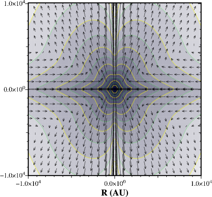
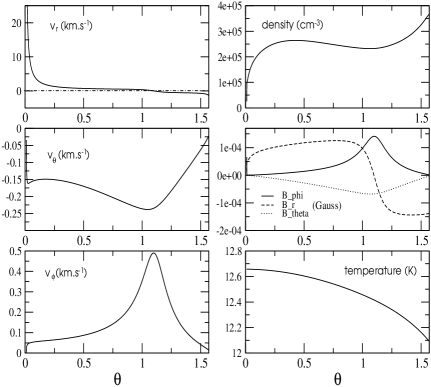
Figure 4: Same as Fig. 3 but for a MHD solution with pure transit. For this particular solution, the initial values of the dimensionless variables are: $u_{r}=1.45\times 10^{3}$, $u_{\theta}=-8.12\times 10^{-2}$, $u_{\phi}=7.49\times 10^{-3}$, $y_{p}=5.12\times 10^{5}$, $y_{\phi}=5.81\times 10^{-1}$, $\mu=5.93\times 10^{-6}$, $\Theta=2.13\times 10^{-1}$ and $f_{\theta}=1.353$. The value of $\alpha$ is -0.22 and the opacity parameters correspond to the dust case $a=0$ and $b=2$.

As previously, the radial velocity traces the infalling/outflowing motion of the gas. For this solution, the opening angle is $\theta_{\rm open}=1.1\;{\rm rad}\approx 60^{\circ}$, where $v_{r}$ changes sign. However, between 1.1 and 0.3, the radial velocity is positive but very small and it is only beyond 0.3 rad $\approx 17^{\circ}$ that a non negligible outflowing motion is occurring.

The outflow velocity is typically 10-20 km s^-1 for the most collimated part and the number density varies from $10^{5}$ to $4\times 10^{5}$ cm^-3 between $0<\theta<\pi/2$. These values fit in the range of typical values of molecular outflows (Bachiller, 1996). The turning angle is the preferential angle for the toroidal magnetic field (middle right panel), responsible of the collimation of the flow via the $j_{z}\times B_{\phi}$ component of the Lorentz force. In consequence, $v_{\theta}$, which traces the movement of the gas towards the axis, is also maximised at the turning point. Naturally, this correlation was not found in the HD case where the opening angle was very small but $v_{\theta}$ was maximum around 55 ^∘. Remembering that $B_{\phi}\propto v_{\phi}$ in the model, $v_{\phi}$ behaves identically to the toroidal field.

The density (upper right panel) presents a strong poloidal gradient ($\partial_{\theta}$) near the rotational axis, followed by an almost constant behavior for intermediate values of $\theta$ and finally increases again when approaching the equatorial region. The strong gradient near the axis contributes to the acceleration of the outflowing material in this region. This behaviour is not present in the HD solutions. The density structure of the present MHD solution appears oblate with respect to the rotational axis whereas it looks prolate for the hydrodynamical model. Such a geometrical difference may be observationally distinguishable at high resolution. Indeed Motte & André (2001) have investigated the morphologies of Class 0 and 1 protostellar envelopes and have found that several sources (e.g. L1527, B335) have elliptical (or even more complex) density structure. They invoke the presence of bipolar outflows to possibly be the reason of these asymmetries. This could be the case in our model.

As in the hydrodynamical case, the temperature is almost constant over the domain. However, the radiative flux plotted in the poloidal plane in Fig. 5, right panel, shows a strong anisotropy and is the highest in the axial zone and also contributes to the acceleration of the outflowing gas. On the other hand, the flux appears smaller in the equatorial region than elsewhere, emphasizing that the equator is a privileged region for the accretion of matter onto the central protostar. That is not the case for the HD model (Fig. 5, left panel) where the radiation is almost spherical.

The typical values for two models, hydrodynamical and magnetized, are gathered in Tab 1 which summerizes the previous points.

	$v_{r}^{\rm out}$ (km.s-1)	$v_{\theta}^{\rm max}$ (km.s-1)	$v_{\phi}^{\rm max}$ (km.s-1)	$\rho_{\rm out}$ (cm-3)	$\rho^{\rm axis}/\rho^{\rm eq}$	$F_{\rm rad}^{\rm axis}/F_{\rm rad}^{\rm eq}$
with B field	$\sim 10$	0.25	0.5	$2\times 10^{5}$	0.25	4.3
no B field	$\sim 1$	0.45	$5\times 10^{-3}$	$1\times 10^{7}$	2	0.5

Table 1: Comparison between typical values of the HD and MHD solutions at a distance of 5000 AU from the central protostar.

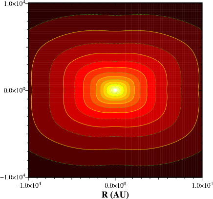
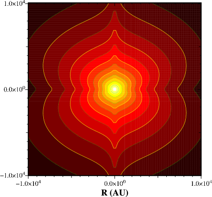
Figure 5: The radiative flux contours of typical transit solutions in the HD (left) and MHD (right) case between 0 and $10^{4}$ AU. At 5000 AU, the typical values are respectively $6\times 10^{3}$ and $3\times 10^{3}$ erg s^-1 cm^-2.

Knowing the velocity and the density for every angle $\theta$ at a fixed radius R, it is possible to calculate mass rates. In particular, the infall mass rate is given by

$$\dot{M}_{\rm in}=2\times 2\pi R^{2}\int_{\theta_{\rm open}}^{\pi/2}v_{r}(R,\theta)\rho(R,\theta)\sin\theta{\rm d}\theta$$ (20)

where $v_{r}(R,\theta)$ and $\rho(R,\theta)$ takes the form of Eq.(10) and Eq.(7). The first factor 2 is present to take into the contribution to the infall from the other side of the equatorial plane.

We compute the infall rates for different central masses and plot the result in Fig. 6. Three solutions are treated: the one detailed previously in Fig. 4 (solid line) and two extreme cases (a low and a high density solutions, in dotted lines). The low and high density solutions are extreme in the sense that they are at the limit of the observational range but not a limit of the model (which can also produce denser or lighter solutions). Then, for a given central mass, our model predict infall rates located between the two dotted lines.

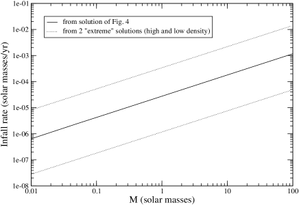
Figure 6: Influence of the central mass on the infall rate for a MHD transit solution. The solid line corresponds to the specific solution presented previously. The dotted lines correspond to two “extreme” solutions of high and low density.

First of all, the infall rate increases with the mass of the protostar and we get a typical value of $\dot{M}_{\rm in}\approx 3\times 10^{-6}$ $M_{\odot}$ yr^-1 for a 0.1 $M_{\odot}$ central object, which is in agreement with rates inferred from observations of low mass YSO (Bontemps et al., 1996). It is important to mention here that the increase of the central mass does not correspond to the temporal evolution of the mass of the protostar: we are studying a self-similar steady-state problem where the central mass is a dimensional parameter. Observationally, the higher the central mass is, the later in the pre-stellar evolution the protostar is, and as a consequence, the lower its accretion rate is. Here we are just studying the influence of the central mass on a given model and the increase of the infall rate is a consequence of the increase of the gravitational force from the source.

The infall rate scales with $M$ following a power-law. For this example, we have $\dot{M}_{\rm in}\propto M^{0.81}$. This behavior comes from the self-similar form we use for the variables and, injecting Eq.(7) and Eq.(10) into Eq.(20) and using Eq.(18) for $r_{0}$ , one finds

$$\dot{M}_{\rm in}\propto M^{\frac{3}{2}}M^{-\frac{2(a+b-1/2)}{5+6a+2b}\left(5/2+2\alpha\right)}\;.$$ (21)

If $a=0$ and $b=2$ (dust case), it simply reads $\dot{M}_{\rm in}\propto M^{\frac{2}{3}(1-\alpha)}$ and with $\alpha=-0.22$ we find a slope of 0.81. In our model the smallest value $\alpha$ can tend to is $-1/2$ ($\alpha=-1/2$ corresponds to pure radial infall) which would give a maximum slope of 1, $\dot{M}_{\rm in}\propto M$ in the dust dominated regime.

With the purely transit solutions like the previous one, the infall rate we calculate corresponds to the rate of gas moving towards the protostar. However, there is no net infall onto the central object in the sense that for these models, all the matter that falls is deflected in the outflow. This can be shown by writing the continuity equation Eq.(1) in the dimensionless variables and integrating over all space:

$$\int_{0+\epsilon}^{\pi/2-\epsilon}\left[(1+2\alpha)\mu u_{r}+\frac{1}{\sin\theta}\frac{{\rm d}}{{\rm d}\theta}(\mu u_{\theta}\sin\theta)\right]\sin\theta{\rm d}\theta$$

$$=0$$ (22)

The first term corresponds to the total dimensionless mass rate over the entire domain. With our boundary conditions $u_{\theta}(0)=u_{\theta}(\pi/2)=0$, and $\mu$ finite, the integration of the second term equals zero. As a consequence, the total mass rate in the model is also equal to zero and all the infalling matter in diverted outward. In order to compare to observations, it is possible to compute the outflow to infall rate ratio, $f=\dot{M}_{out}/\dot{M}_{in}$. For Class 0 and 1 objects, the ratio is found to be smaller than unity typically, $f\sim 0.1-0.3$ (Bontemps et al., 1996; Richer et al., 2000). In our case, for pure transit models, $f=1$ by construction since all the material that is coming in has to be rejected in the outflow.

Nevertheless, the inclusion of magnetic field greatly improves the properties of the solutions which now compare well with observational quantities, with fast, collimated outflows.

4.2 Dust case – a typical solution with net infall

We now present solutions with a combination of transit and pure infall solutions similarly to Lery et al. (2002). We briefly review the interest and the properties of such solutions.

The method of integration is the same as previously except that, here, the domain is separated in two zones. The separation occurs at the angle $\theta_{s}$. From $\theta_{0}$ to $\theta_{s}-\epsilon$, we search for a transit solution, qualitatively identical to the one of the previous section. From $\theta_{s}+\epsilon$ to $\pi/2-\epsilon$, we look for a solution that presents the characteristic of an infall ($v_{r}<0$) but that is directed toward the equator and not toward the axis so that the gas is not deviated. This condition is fulfilled if the $\theta-$velocity is positive. At the end of the transit region, in $\theta_{s}$, $v_{\theta}$ tends to zero and is negative (requirement for transit). To integrate the system in the net infall region, we change the sign of $v_{\theta}$, in order to get a strictly infalling pattern and use the end values of the transit solution, as initial conditions for the solution between $\theta_{s}$ and $\pi/2$.

There is a small region around $\theta_{s}$ which is not treated: $\theta=\theta_{s}$ is a location that cannot be reached (as for the equator in the pure transit solutions) and the integration numerically failed before reaching it. It is also important to mention that the two solutions, on both sides of $\theta_{s}$ are mathematically independent. The continuity set between the two zones is in consequence only apparent.

A solution with the characteristics described above is shown in Fig. 7. As previously, we plot the density contours and the velocity field (left panel) as well as the variation of the physical quantities with $\theta$ at a given radius (right panel). We are considering the standard case for which the opacity is dust-dominated.

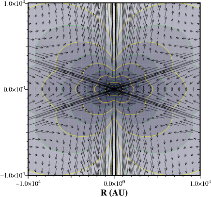
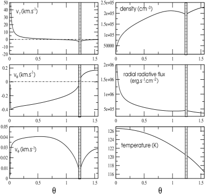
Figure 7: Same as Fig. 4 but for a solution with net infall.

The two zones can be distinguished: i) the transit zone, characterized by the change of the sign of the radial velocity and by a negative theta-velocity. (i.e. from $\theta_{0}=10^{-2}$ to $\theta_{s}\sim 0.8$ rad), ii) a net infalling region where $v_{r}<0$ and $v_{\theta}>0$ in the remaining of the domain. In this region, the gas is falling onto the equatorial plane so it can eventually accrete onto the central protostar. The untreated region between the two zones has been shadowed.

Fig. 7 shows a solution with an opening angle of $\theta_{\rm open}\sim 30^{\circ}$ but solutions with smaller opening angles have also been found. The radial velocity for the outflow is 20-50 km s^-1 and the average density around $2\times 10^{5}$ cm^-3. Again, the solution appears almost spherical: each physical quantity does not show strong gradient except close to the boundary angles. Identically with the transit magnetized solution, the minimum density and maximum radiative flux is in the axis region: this allows the outward acceleration of the gas in this region and the radial velocity is then also maximum at the axis.

The $\theta-$velocity tends to zero at the axis and towards $\theta_{s}$. These are the boundary conditions we require for transit solution and have in consequence to establish a pressure balance between the transit and net infalling regions. Near the equator, $v_{\theta}$ does not tend to zero. This implies that the equatorial zone $[\pi/2-\epsilon,\pi/2]$ has to be seen as a sink that absorbs anything entering it. Looking at Eq.(22) for the net infalling zone (i.e. integrating between $\theta_{s}$ and $\pi/2$), one sees that a non-zero $v_{\theta}$ at one of the boundary ($\pi/2$ in the present case) results in a non-zero global mass rate in the considered region. This justifies a posteriori terming these solutions “net infall” models. For this category of models, the ratio $f$ is then smaller than unity. For the particular solution shown here, $\dot{M}_{\rm out}\sim 2\times 10^{-5}$ M_⊙ yr^-1 and $\dot{M}_{\rm in}\sim 2\dot{M}_{\rm out}$ resulting in $f=\dot{M}_{\rm out}/\dot{M}_{\rm in}\sim 0.5$. This is a typical value for net infall models, but larger and smaller values can also be obtained by setting the net infalling region as a smaller or larger fraction of the full model.

4.3 Influence of opacity

The solutions presented previously had a dust-dominated opacity. This is the situation in the present-day universe which is enriched in heavy elements, molecules and grains thanks to many generations of stars and stellar nucleosynthesis. However, in the primordial universe, star formation occurred in an almost metal-free environment where the chemical composition was a mixture of hydrogen (H), helium (He) and very small traces of deuterium (D) and light elements (Li, Be, B). To understand the physics in the early universe, it is necessary to have accurate values of its opacities. Many studies undertaken on primordial star formation used only the species involved in the formation of molecular hydrogen (and sometimes helium) (Stahler, 1986; Omukai & Nishi, 1998; Nakamura & Umemura, 1999) as H₂ is the most abundant molecular species formed under primordial condition and is also the most effective coolant of the gas in the low temperature regime of star formation. However, HD molecules can also contribute to the cooling of the gas when H₂ becomes inefficient (Palla, 1999) and in a recent paper, Mayer & Duschl (2005) show that the inclusion of Li in primordial opacity calculation lead to significant changes, up to two orders of magnitude for $T<4000$ K and conclude that the influence of Li on the different stages of population III star formation and evolution could be assessed. Here, we wish to study the behavior of our models when the optical properties of the fluid are those of a dust-free environment.

The use of the Kramer’s law form for the opacity prevents an explicit treatment of the cooling that includes all the species previously mentioned. However, the Kramer’s opacity coefficients ($a,b$) can be interpreted in term of the physical process enabling the cooling. The emission rate per unit of volume can be written as $\epsilon=4\sigma\rho\kappa T^{4}\propto\rho^{a+1}T^{b+4}$ (Boily & Lynden-Bell, 1995).

• $a=0$ corresponds to situations where a single efficient component (dust or $CO$) dominates the cooling, assuming its fraction by mass remains constant during evolution.

• On the other hand, $a=1$ gives the density dependence of the opacity when the cooling is due to two-particle processes and no coolant is dominant. For such a density dependence, the system is expected to be dilute and cold so that the excitation levels are almost empty.

• $b$ measures the difference between a black body emission ($\propto T^{4}$) and the one considered here. In the case of dust, $b=2$ as seen before. This appears to be an upper limit and $b$ then decreases for other types of cooling, in particular $b\in[-5/2,-1]$ for molecular cooling in interstellar clouds (Goldsmith & Langer, 1978).

In order to study the influence of the opacity on the solutions of our model, we start from the dust case and then increase $a$ from 0 to 1 and decrease $b$ from 2 to 1 so as to leave the dust-dominated regime. If no dust is present in the star formation environment, then the main source of opacity would come from molecular line cooling . As mentioned previously, that case would see $b$ in the range $[-5/2,-1]$. However, in this work, $b$ does not take any value smaller than unity. This is due to the stiffness of the ODE system to solve. In fact, to study the influence of opacity on the solutions, we do not change any other parameters but $a$ and $b$; for a given set of input parameters, a valid solution (i.e. filling the whole space and presenting circulation features) appears to remain valid only for $b$ varying between 2 and 1. Below 1, the integration fails before $\theta=\pi/2$ and the other input parameters should be slightly adjusted. Doing so would make it impossible to distinguish the effects due to opacity from those coming from the new input values. The limit $b=1$ is not strict, we found solutions that could still be integrated with $b\lesssim 1$ and others that would fail earlier.

By changing $a$ and $b$ progressively, we depart from the dust-dominated regime. It is however important to note that we cannot say what type of coolant it is we are modelling except that it is less efficient than dust and results in a smaller opacity.

The study is made on pure transit solutions only and not on net infall ones as the discontinuity between the two regions of the latter was more difficult to handle.

The results are shown in Fig. 8 and Fig. 9. The infall rate is calculated in the same way as in Sect. 4.1 and is plotted in Fig. 8 as a function of the Kramer’s opacity parameter $a$ ($b$ stays equal to 2). The infall rate increases as one leaves the dust opacity regime. Very simply, when the opacity decreases and the medium becomes more transparent, the photons escape more easily and are less efficient in slowing the infalling gas.

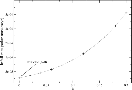
Figure 8: Influence of Kramer’s opacity parameter $a$ on the infall rate.

In Fig. 9, the left panel represents the density for different sets ($a,b$). The radial radiative fluxes are plotted on the right panel for the same sets of parameters. Furthermore, the quantities plotted are dimensionless (i.e., $\mu(\theta)$ and $f_{r}(\theta)$) because as $a$ and $b$ are modified, the fiducial scale $r_{0}$ changes (see Eq.(18)): the influence of the opacity on the morphology of the solutions would be more difficult to visualize as they would not start from the same point.

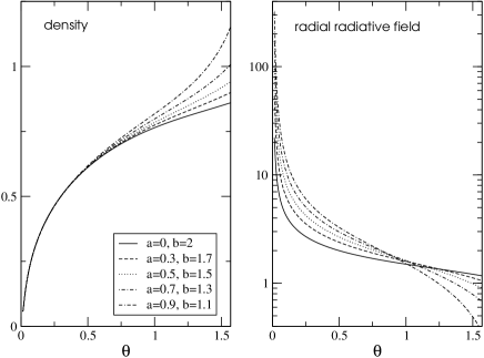
Figure 9: Influence of the opacity parameters $a$ and $b$ on the dimensionless density and radial radiative flux.

The dimensionless density increases in the equatorial region as one leaves the dust-dominated regime. As it is the dimensionless density, this means that as $a$ increases and $b$ decreases, the ratio between the density at the equator and at the rotational axis increases. The radial radiative flux shows the opposite behavior: the flux is relatively smaller at the equator than in the axial region.

It is not possible to generalize this behavior as not all the solutions that were found behave like that. For example, the morphology of the solution presented in Sect.4.1 was almost unaffected by the change of opacity. The only difference was observed for its dimensional quantities that would scale differently and, as a result, give a higher infall rate when dust is not the dominant coolant (see Fig. 8). However, it is of interest that such solutions exist: the higher density in the equatorial region along with the weaker radiative field in this region could lead to the accumulation of matter in the equatorial plane (i.e., to a more massive accretion disk) and may ultimately lead to the formation of more massive star for dust-free opacity regimes (such as the ones of the primordial universe).

5 General properties of MHD models

The main feature of the model is the production of a heated pressure-driven outflow with magneto-centrifugal acceleration and collimation. An evacuated region exists near the axis of rotation where the outflow is produced and the density systematically increases with the angle from the axis. The streamlines passing close to the rotational axis are also the ones closest to the central object (see Fig. 11, upper left panel). The gas on these streamlines transits deeper in the gravitational well and is also the most vigorously heated. As a consequence, the radial velocity of the outflow is always maximum near the axis and decreases with increasing poloidal angle $\theta$.

5.1 Two families of solutions

All the solutions that we have found have the same qualitative properties, except around their turning point. In this region, two distinct families of solutions appear as shown in Fig. 10. The rotational velocity $v_{\phi}$ (left panel) and the radial magnetic field $B_{r}$ (right panel) are plotted as a function of the poloidal angle $\theta$ for different solutions.

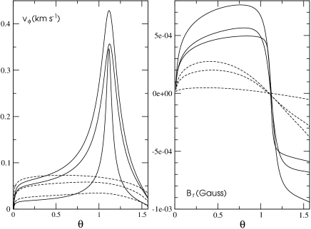
Figure 10: The rotational velocity (left) and radial magnetic field (right) plotted as a function of $\theta$. The continuous and dotted lines correspond to the two types of solutions. For clarity, we only show solutions with almost the same turning angle, but others were found.

The solutions fall into one of the two categories: i) slow rotators where the rotational velocity is small and almost constant over the entire domain (dotted line) and ii) fast rotators where $v_{\phi}$ increases and decreases with a strong gradient around the turning point of the solution (solid line). At its maximum, $v_{\phi}$ peaks at about four times the $v_{\phi}$ value of the other solutions. Because we have $B_{\phi}\propto v_{\phi}$, the solutions that peak at the turning point also have a much stronger toroidal field there and as a consequence a larger pinch force towards the rotational axis.

The radial magnetic field (Fig. 10, right panel) changes sign at the turning point of the solution ($B_{r}\propto v_{r}$) and it appears that the fast rotating solutions (solid lines) have a substantially higher radial magnetic field on the overall domain than the slow rotating models (from 2 to 16 times higher for the solutions shown).

The other variables (not shown here: density, temperature, etc…) do not seem to be affected and no distinction can be made between the two types of solutions when looking at these quantities. No morphological differences appear between the two types of models and the density profiles all indicate the characteristic oblate shape of magnetized solutions. Rotation and magnetic field seem coupled and the solutions with reasonable dimensioned quantities are in one of the two following categories: i) slow rotating and poorly magnetized or ii) faster rotating and highly magnetized.

5.2 Energetics of the solutions

In order to compare and contrast the two families of solutions, the evolution of the energy along a streamline is considered. We call Family 1/Family 2 the slow/fast rotating weakly/strongly magnetized family of solutions found in the previous section.

Streamlines follow ${\rm d}r/(r{\rm d}\theta)=u_{r}/u_{\theta}$ in the poloidal plane. It is convenient to look at the local specific energy components normalized to the local specific gravitational energy (to have a dimensionless quantity) and to define their sum as

$$Be(r,\theta)\equiv-\frac{1}{E_{\rm grav}}\left(E_{k}+E_{\rm grav}+\frac{p}{\rho}+E_{\rm magn}\right)$$ (23)

where $E_{k}$ is the specific kinetic energy, $E_{\rm grav}=-GM/r$ the specific gravitational potential energy, and $E_{\rm magn}=B^{2}/8\pi\rho$ the specific magnetic energy. Using the self-similar form for the quantities, $Be$ becomes

$$Be(\theta)=\frac{1}{2}\left(u_{r}^{2}+u_{\theta}^{2}+u_{\phi}^{2}\right)-1+\Theta+\frac{1}{8\pi\mu}\left(\frac{u_{p}^{2}}{y_{p}^{2}}+\frac{u_{\phi}^{2}}{y_{\phi}^{2}}\right)$$ (24)

Note that in the hydrodynamical case, the Bernoulli theorem implies that $Be$ is constant along a streamline.

In Fig. 11, upper left panel, streamlines are plotted for two solutions, one from each family. The central object is located at the origin. It is interesting to note that for streamlines integrated from the same point (located in the outflowing region), the solution from Family 2 transits closer to the central object, deeper in the gravitational well than the one from Family 1. This is a general trend that has been observed for many solutions. The three other panels in Fig. 11 show energy components plotted along these two streamlines.

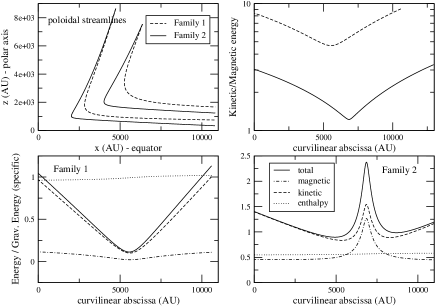
Figure 11: Family 1 and 2 refer respectively to the slow and fast rotating solutions found previously. Upper left: poloidal streamlines. Upper right: ratio of the kinetic to the magnetic energy as a function of the curvilinear abscissa $s$. $s=0$ is chosen at the infalling end of the streamline. Lower left: energetics of a solution along a streamline for a solution from Family 1. The specific energy components have been normalized to the gravitational potential energy. Lower right: same as lower left for a solution from Family 2.

On lower left and right panels the different specific energy components as a function of the position along the streamline of the solution from Family 1 and 2 are plotted. The origin of the curvilinear abscissa $s$ is chosen at the “infalling end” of the streamline.

Far from the turning point, the main contribution to the kinetic energy ($E_{k}$) comes from the radial velocity $v_{r}$ ($v_{\theta}$ and $v_{\phi}$ have much smaller values). The absolute value of $v_{r}$ rapidly decreases when approaching the turning point (See Fig. 4) and so does $E_{k}$ (dashed line), for both Family 1 and 2 solutions. Near the turning point, however, the contribution of $v_{\theta,\phi}$ to $E_{k}$ becomes dominant: i) for the slow rotating solutions (Family 1 – lower left panel), $v_{\phi}$ does not change much on the domain and $E_{k}$ reaches a minimum at the turning point, ii) but for the fast rotators (lower right), $v_{\phi}$ quickly increases at the turning point and $E_{k}$ reaches a local maximum. The magnetic energy qualitatively follows the same behavior as $B_{r,\theta}\propto v_{r,\theta}$ and $B_{\phi}\propto v_{\phi}$.

Finally, the ratio of the kinetic to the magnetic energy is plotted on the upper right panel in Fig. 11, again for the two types of solutions. Qualitatively, they behave alike, and $E_{k}/E_{\rm magn}$ is in both case minimum at the turning point. This conforms with intuition as one expects a larger influence of the magnetic field near the central protostar. However, at the turning point, $E_{\rm magn}$ is 5 times smaller than $E_{k}$ for the slow rotating solution while it is comparable to $E_{k}$ for the fast rotating model. For clarity only two solutions have been plotted here, but it has been found a general behaviour that $(E_{k}/E_{\rm magn})^{\rm Family2}_{\rm turn.}\sim 1$. Furthermore, the same ratio for Family 1 solutions has been found many times much greater (5-100) than unity.

In conclusion, the behaviour of the two types of solutions is similar far from their turning point, but then differs significantly: for the slow rotating models, the magnetic energy is always much smaller than the kinetic energy whereas they become comparable for the fast-rotating solutions. The magnetic field appears then to be responsible for a closer transit around the center of the latter ones. Despite this difference between the two families of solutions, the properties (velocity, density) of the outflows they power are similar.

6 Discussion

6.1 Behavior at large distance

After the main early phase where infall dominates the dynamics, the protostar deposits linear and angular momentum and mechanical energy into its surroundings through its jets and molecular outflow. It is therefore important to discuss the behavior of the outflows at large distance. In the case of low mass stars, the accretion-ejection engine should dominate the global dynamics and produce relatively weak molecular outflows. In that case, the present model may apply only for a short stage at the earliest phases of low mass star formation. On the other hand, if the physics of the outflow formation remains the same regardless the mass of the protostar, the dynamics of massive objects should be dominated by the transit and should have strong and heavy molecular outflows, according to the present model. In that case, the transit model plays a major role in the formation of massive stars. Moreover, the transit model brings an interesting new feature for the interaction between molecular outflows and jets. Indeed, a lot of gas is brought to the axial region that is not at rest and is already stratified when the atomic jet starts propagating away from the protostar. It will drastically change the jet propagation and stability properties. This demonstrate the importance of understanding of the history of outflows in order to model correctly the behavior of jets.

Also, according to our model, at larger distance, $\rho\propto r^{2\alpha-1/2}$, $B\propto r^{\alpha-3/4}$, and $v\propto r^{-1/2}$. The magnetic field and the density decrease faster than the velocity. For example for $\alpha=-1/4$, $\rho\propto r^{-1}$, $B\propto r^{-1}$, and $v\propto r^{-1/2}$, and the outflow becomes purely ballistic (Lery et al., 2002). Only large bow-shocks due to the long time-scale variations of the source should survive. Ultimately, the combined effects of the reduction of the ionization and temperature in the giant bows, and of the lack of ambient medium, may make the outflows fade out and finally become very difficult to observe on distances of 3 to 10 pc. However, the momentum that they may transfer to the ambient medium could help to maintain turbulence on large scales.

6.2 The outflow evolution

Of our steady-state model, any temporal evolution is beyond the scope. However, we may speculate on the evolution of YSOs by considering the slow quasi-steady evolution of our model. With the new insight given by the model, we suggest some physical justifications for the early evolutionary sequence of both low and high mass YSOs which is usually defined on the basis of an empirical scheme only.

During the Class 0 stage, most of the mass of the system is still located in the infalling envelope. The source is totally embedded and the transit of matter around the center object can start during the formation of the stellar core. This gives rise to a fast, powerful and collimated molecular outflow. However during this early stage, the central object may not have already developed the jet that is commonly thought to drive the molecular outflow.

When reaching the early Class 1 stage, the central object is surrounded by both a disk and a diffuse circumstellar envelope. A jet eventually emerges from the newly formed inner accretion disk as the transit continues. The jet may then pressurize and entrain the material in the axial region, pushing the transit flow away from the axis, thus reducing the molecular outflow velocity and increasing its diameter. Therefore, molecular outflows will appear to be less powerful and less collimated with time.

For low mass protostars, in the latest stages of the pre-stellar evolution, the central object should not be embedded in an envelope and our model cannot apply. The molecular outflow continues to spread out and slow down and is eventually overtaken by the central jet still fed by the accretion disk. In the case of high mass stars, the transit features may remain in action until the central star forms and reach the main sequence. Either the increasing opening angle of the molecular outflow in the low mass case, or the ignition of the central object may ultimately stop the accretion by suppressing any contact between the reservoir formed by the molecular cloud and the accretion disk or the star.

7 Summary

In this paper, we have presented a MHD model that applies to infall and molecular outflows around young stellar objects. The model is based on the radial self-similarity assumption applied to the basic equations of ideal, axisymmetric and steady-state MHD, including Poynting flux. Instead of the usual mechanisms invoked for the origin of molecular outflows (underlying jet or wind), the outflow is powered by the infalling matter through a heated quadrupolar transit pattern around the central object.

Solutions without magnetic field have been found and they appear almost spherical (quantities do not vary much with the poloidal angle). Although they do not compare well with observation ranges (too dense and too slow outflow), they indicate that thermodynamics is a sufficient engine to generate an outflow. They could apply to star formation in the primordial universe or in the very early stage of star formation where magnetic fields may not be dynamically important (however, in the latter case, the point mass gravity field should be replaced by self-gravity).

The magnetized solutions show dynamically significant density gradients in the axial region, precisely where the radial velocity and collimation are the largest. Their radiative field is also highly anisotropic and the highest at the rotational axis. It contributes to the ejection of the gas. Quantitatively, the pure transit solutions compare well with observations of outflows: velocities of a few tens of km s^-1 and typical density of $10^{4-5}$ cm^-3.

However, for these models all the infalling gas is deviated into the outflow – there is no net infall. It is possible to obtain, from the same set of equations, a purely infalling region around the equatorial plane. The gas in this region is not deviated and will likely end up on the accretion disk around the protostar. When changing the scaling and putting a more massive central object, the infall rate also increases. This indicates that our model favors the large accretion rate scenario to form massive stars.

The influence of the opacity on the transit solutions has been studied. When leaving the dust dominated regime, the fiducial scale of the model decreases which results in an increase of the infall rate. Furthermore, the morphology of some solutions is also affected: the density ratio between the equator and the axis increases while the radial radiative flux ratio decreases. As a consequence, when dust does not dominate the cooling, such as in the primordial universe, matter could be more easily accumulated in the equatorial region and form more massive stars .

We suggest that molecular outflows are dominated by the global transit of material around the protostar (except for a thin layer surrounding the central jet – if present, where the dynamics is governed by entrainment) and that the same process occurs from low to high mass forming stars. The present work also suggests that radiative heating and magnetic field may ultimately be the main energy sources driving outflows during star formation, at the expense of gravity and rotation.

Finally, although the details of the outflow mechanisms may be peculiar to individual objects we believe the infall-outflow circulation arises naturally given accretion, and thus could also be present in other astronomical objects such as active galaxies and around suitably placed compact objects, such as neutron stars.

References

- André et al. (2000) André, P., Ward-Thompson, D., & Barsony, M. 2000, Protostars and Planets IV, 59
- Bachiller (1996) Bachiller, R. 1996, ARA&A, 34, 111
- Bachiller & Tafalla (1999) Bachiller, R. & Tafalla, M. 1999, in NATO ASIC Proc. 540: The Origin of Stars and Planetary Systems, 227–+
- Barenblatt (1996) Barenblatt, G. I. 1996, in Scaling, self-similarity, and intermediate asymptotics, Cambridge University Press
- Barenblatt & Zel’dovich (1972) Barenblatt, G. I. & Zel’dovich, Y. B. 1972, Annual Review of Fluid Mechanics, 4, 285
- Barsony & Chandler (1993) Barsony, M. & Chandler, C. J. 1993, ApJ, 406, L71
- Beech & Mitalas (1994) Beech, M. & Mitalas, R. 1994, ApJS, 95, 517
- Behrend & Maeder (2001) Behrend, R. & Maeder, A. 2001, A&A, 373, 190
- Blandford & Payne (1982) Blandford, R. D. & Payne, D. G. 1982, MNRAS, 199, 883
- Boily & Lynden-Bell (1995) Boily, C. M. & Lynden-Bell, D. 1995, MNRAS, 276, 133
- Bonnell et al. (1998) Bonnell, I. A., Bate, M. R., & Zinnecker, H. 1998, MNRAS, 298, 93
- Bontemps et al. (1996) Bontemps, S., André, P., Terebey, S., & Cabrit, S. 1996, A&A, 311, 858
- Chan & Henriksen (1980) Chan, K. L. & Henriksen, R. N. 1980, ApJ, 241, 534
- Chandler et al. (1998) Chandler, C. J., Barsony, M., & Moore, T. J. T. 1998, MNRAS, 299, 789
- Chernin et al. (1994) Chernin, L., Masson, C., Gouveia dal Pino, E. M., & Benz, W. 1994, ApJ, 426, 204
- Churchwell (1997) Churchwell, E. 1997, ApJ, 479, L59+
- Churchwell (2000) Churchwell, E. 2000, in Unsolved Problems in Stellar Evolution, 41–+
- Downes & Ray (1999) Downes, T. P. & Ray, T. P. 1999, A&A, 345, 977
- Ferreira (1997) Ferreira, J. 1997, A&A, 319, 340
- Fiege & Henriksen (1996) Fiege, J. D. & Henriksen, R. N. 1996, MNRAS, 281, 1038
- Goldsmith & Langer (1978) Goldsmith, P. F. & Langer, W. D. 1978, ApJ, 222, 881
- Henriksen (1996) Henriksen, R. N. 1996, in Solar and Astrophysical MHD flows, Tsinganos, K. (eds), 567
- Ladd et al. (1991) Ladd, E. F., Adams, F. C., Fuller, G. A., Myers, P. C., Casey, S., Davidson, J. A., Harper, D. A., & Padman, R. 1991, ApJ, 382, 555
- Lee et al. (2000) Lee, C., Mundy, L. G., Reipurth, B., Ostriker, E. C., & Stone, J. M. 2000, ApJ, 542, 925
- Lee et al. (2001) Lee, C., Stone, J. M., Ostriker, E. C., & Mundy, L. G. 2001, ApJ, 557, 429
- Lery (2003) Lery, T. 2003, in Recent Research Developments in Astrophysics, Research Signposts (India), Vol. 1
- Lery et al. (1999) Lery, T., Henriksen, R. N., & Fiege, J. D. 1999, A&A, 350, 254
- Lery et al. (2002) Lery, T., Henriksen, R. N., Fiege, J. D., Ray, T. P., Frank, A., & Bacciotti, F. 2002, A&A, 387, 187
- Mayer & Duschl (2005) Mayer, M. & Duschl, W. J. 2005, MNRAS, 358, 614
- Mihalas & Klein (1982) Mihalas, D. & Klein, R. I. 1982, Journal of Computational Physics, 46, 97
- Motte & André (2001) Motte, F. & André, P. 2001, A&A, 365, 440
- Nakamura & Umemura (1999) Nakamura, F. & Umemura, M. 1999, ApJ, 515, 239
- Norberg & Maeder (2000) Norberg, P. & Maeder, A. 2000, A&A, 359, 1025
- Omukai & Nishi (1998) Omukai, K. & Nishi, R. 1998, ApJ, 508, 141
- Ostriker et al. (2001) Ostriker, E. C., Lee, C., Stone, J. M., & Mundy, L. G. 2001, ApJ, 557, 443
- Ouyed & Pudritz (1997) Ouyed, R. & Pudritz, R. E. 1997, ApJ, 482, 712
- Palla (1999) Palla, F. 1999, in Star Formation 1999, Proceedings of Star Formation 1999, held in Nagoya, Japan, June 21 - 25, 1999, Editor: T. Nakamoto, Nobeyama Radio Observatory, p. 6-11, 6–11
- Pollack et al. (1985) Pollack, J. B., McKay, C. P., & Christofferson, B. M. 1985, Icarus, 64, 471
- Raga & Cabrit (1993) Raga, A. & Cabrit, S. 1993, A&A, 278, 267
- Richer et al. (2000) Richer, J. S., Shepherd, D. S., Cabrit, S., Bachiller, R., & Churchwell, E. 2000, Protostars and Planets IV, 867
- Rodríguez-Franco et al. (1999) Rodríguez-Franco, A., Martín-Pintado, J., & Wilson, T. L. 1999, A&A, 351, 1103
- Semenov et al. (2003) Semenov, D., Henning, T., Helling, C., Ilgner, M., & Sedlmayr, E. 2003, A&A, 410, 611
- Shu (1977) Shu, F. H. 1977, ApJ, 214, 488
- Shu (1991) Shu, F. H. 1991, in ASP Conf. Ser. 20: Frontiers of Stellar Evolution, 23–44
- Shu et al. (1995) Shu, F. H., Najita, J., Ostriker, E. C., & Shang, H. 1995, ApJ, 455, L155+
- Shu et al. (2000) Shu, F. H., Najita, J. R., Shang, H., & Li, Z.-Y. 2000, Protostars and Planets IV, 789
- Snell et al. (1980) Snell, R. L., Loren, R. B., & Plambeck, R. L. 1980, ApJ, 239, L17
- Stahler (1986) Stahler, S. W. 1986, PASP, 98, 1081