Ensemble Learning Independent Component Analysis of Normal Galaxy Spectra

Abstract

In this paper, we employe a new statistical analysis technique, Ensemble Learning for Independent Component Analysis (EL-ICA), on the synthetic galaxy spectra from a newly released high resolution evolutionary model by Bruzual & Charlot. We find that EL-ICA can sufficiently compress the synthetic galaxy spectral library to 6 non-negative Independent Components (ICs), which are good templates to model huge amount of normal galaxy spectra, such as the galaxy spectra in the Sloan Digital Sky Survey (SDSS). Important spectral parameters, such as starlight reddening, stellar velocity dispersion, stellar mass and star formation histories, can be given simultaneously by the fit. Extensive tests show that the fit and the derived parameters are reliable for galaxy spectra with the typical quality of the SDSS.

1 Introduction

With the coming of large sky area spectroscopic surveys, the first decade of the $21^{st}$ century turns into the golden age for extragalactic astronomy. The ongoing SDSS (the Sloan Digital Sky Survey, York et al. 2000) and the forthcoming LAMOST (the Large Sky Area Multi-Object Fiber Spectroscopic Telescope, Chu & Zhao 1998) are now and will be providing us millions of high quality optical spectra for both normal and active galaxies. For the first time it becomes doable to explore the spectral properties of a great diversity of galaxy populations. Strong constraints can be set on various scenarios of galaxy formation and evolution by comparing the measured quantities with theoretical predictions. However, full exploitation of such large data sets demands for the development of new methods that can extract the spectral characteristics of individual galaxies reliably, consistently, and efficiently.

In optical band, an observed galaxy spectrum is the combination of starlight, nebular emission lines, and/or nuclear emission. Proper interpretation of the stellar spectrum is essential to study the galactic properties, such as dust contents, stellar velocity dispersion, metallicity, and star formation histories. Nebular emission lines are produced in the HII regions around young, massive (OB) UV-emitting stars, and are important tools for studying star formation and chemical evolution in galaxies. They are often heavily entangled with stellar absorption features, especially in weak emission line galaxies. Hence the proper decomposition of emission lines and starlight components is required toward a physical interpretation of a galaxy spectrum (e.g., Tremonti et al. 2004). Proper stellar subtraction is also essential for the study of AGN emission lines if contaminated by the stellar absorption lines (e.g., Hao et al. 2002).

Many attempts have been made to fit the galaxy spectra in the past decades. For those who are only interested in emission line properties, the spectra of absorption line galaxies were generally used as templates to fit the emission line free region of galaxy spectra (e.g., Filippenko & Sargent 1988). The “pure line spectrum” can then be obtained by subtracting the best fitting spectrum. The drawback of such an approach is obvious, since the stellar content of an emission line galaxy under study is often quite different from that of an absorption line galaxy. Improvements have been made along this direction ever since. For instance, Ho, Filippenko, & Sargent (1997) used an objective algorithm to find the best combination of galaxy spectra to create an “effective” template. The use of a large basis of input spectra ensures a closer match to the true stellar population. Recently, Hao et al. (2005) applied Principle Component Analysis (PCA, Madgwick et al. 2002 and references therein) to several hundred pure absorption line galaxies and chose the first 8 eigen-spectra as the templates. This approach can greatly reduce the computational time of the fit, and is ideal for fitting large data sets like the SDSS.

To study the stellar contents reside in unresolved galaxies requires the so called stellar population analysis. Two different approaches have been adopted for this purpose: empirical (e.g. Pelat 1997; Cid Fernandes et al. 2001) and evolutionary population synthesis (pioneered by Tinsley 1967). The empirical population synthesis uses the observed spectra of stars and star clusters to model a galaxy spectrum. However, this method is limited by the coverage range of the observed stellar library. The evolutionary population synthesis is a more direct approach in theoretical aspect. In this scheme, the age- and metallicity-dependent modelled spectra of stellar systems are built with physical input parameters, such as the Initial Mass Function (IMF), the Star Formation Rate (SFR) and, in some cases, the rate of chemical enrichment. The limitations of evolutionary population synthesis models used to arise from the uncertainties in its two principal building blocks: stellar evolution models and spectral libraries. Great advances have been achieved in both aspects in recent years (Charbonnel et al. 1999; Girardi et al. 2000; Le Borgne et al. 2003). The most up-to-date release of a high spectral resolution stellar evolutionary synthesis model by Bruzual & Charlot (2003, hereafter BC03), which incorporates these progresses, provides a library of Simple Stellar Populations (SSPs). This spectral library enables accurate studies of stellar populations in galaxies for the first time.

The BC03 library has been employed by several groups to decompose galaxy spectra into various number of SSPs of different ages and metallicities. To reduce the computational expense, either a compressed version of the spectrum in study is used (BC03), or a few SSPs are selected as templates (Tremonti et al. 2004). We note that recent improvement in the statistical analysis technique may help. In this work we adopt a rather different approach grounded on Independent Component Analysis (ICA) to model galaxy spectra. The most prominent earmark of this method in comparison with previous ones is that it works without any a-priori knowledge on the galaxy spectrum analyzed.

The first astrophysical application of ICA is the Cosmic Microwave Background analysis (Baccigalupi et al. 2000) and it has subsequently been implemented in this research area by several authors (e.g. Maino et al. 2002; Moudden et al. 2004). We present here the application of a new ICA algorithm—Ensemble Learning for ICA (EL-ICA )—first proposed by Lappalainen (1998) and later on generalized by Miskin & MacKay (2001), to the spectral library of synthetic galaxy spectra from BC03 and the spectral features of the SDSS galaxies. The robustness and high efficiency of the new method make it a viable technique for enormous data sets of normal galaxy spectra, including type 2 AGN (Active Galactic Nuclei). Its application to decompose stellar and nuclear components in the spectrum of type 1 AGN will be explored in forthcoming papers.

This paper is organized as follows. In §2 below, ICA method is briefly introduced and EL algorithm is explained. §3 applies the EL-ICA method to the synthetic galaxy spectra from the evolutionary models of BC03 SSP and derives our galaxy templates. In §4, we implement these templates to analyze the galaxy spectra in the SDSS Data Release 2 (DR2). The reliability of the obtained spectral parameters is carefully inspected in §5. Our conclusions are summarized in the last section. Throughout this paper, a $\Lambda$-dominated cosmology with $H_{0}=70~{}km~{}s^{-1}~{}Mpc^{-1}$, $\Omega_{M}=$ 0.3 and $\Omega_{\Lambda}=$ 0.7 is assumed.

2 Ensemble Learning Independent Component Analysis

Here we only recall the fundamental concepts of ICA and the essential features of EL algorithm. Readers who are interested in ICA and EL method may refer to Hyvärinen et al. (2001) and Miskin & MacKay (2001).

2.1 Independent Component Analysis

First introduced in the early 1980s and widely used in the late 1990s, ICA is a new Blind Source Separation (BSS) method for finding statistically independent underlying components from multidimensional statistical data. ICA can be defined as follows: Given a set of observations of random variables $f^{j}(\lambda),~{}j=1,2,...,m$, where $\lambda$ is sample index (here we take $f^{j}(\lambda)$ as the spectrum of a stellar system and $\lambda$ the wavelength), we can assume that they are a linear combination of a number of Independent Components (ICs),

$$f^{j}(\lambda)=\sum_{i=1}^{n}a^{j}_{~{}i}IC^{i}(\lambda)+N^{j}(\lambda)$$ (1)

where $a^{j}_{~{}i}$ is $m\times n$ mixing matrix of unknown coefficients and $N^{j}(\lambda)$ is the noise of $f^{j}(\lambda)$. The task of ICA is to estimate both the unknown combining coefficients $a^{j}_{~{}i}$, the noise $N^{j}(\lambda)$ and the $IC^{i}(\lambda)$ from $f^{j}(\lambda)$ only based on the statistical independence among $IC^{i}(\lambda)$.

As a useful statistical and computational technique, ICA can be taken as an extension to Principle Component Analysis (PCA), but much more powerful. In many cases, ICA can find the underlying factors when PCA fails completely. The reason lies in two aspects: 1) Independence is much more stronger than uncorrelatedness. PCA always finds eigen-vectors (or PCs) grounded on the fact that they are uncorrelated, but uncorrelatedness is often not enough. 2) Orthogonality is invalid for a general mixing process. ICA model does not require the underlying factors are orthogonal while PCA does. Nonlinear de-correlation is the basic method to find ICs. Many methods have been developed for estimating the ICA model and all of these methods use some form of high-order statistics.

2.2 Ensemble Learning for ICA

It has been shown that the EL algorithm can be applied to ICA model (Lappalainen 1998). In information theory, entropy is measure of uncertainty and it can be used as a measure of the quality of our models. Suppose we don’t know the distribution, $p(\Theta)$, and our model is $q(\Theta)$, the relative entropy, $d_{KL}(q||p)$, is a measure of how different the two probability distributions (over the same event space) are. We can minimize $d_{KL}(q||p)$ to have a probabilistic model as accurate as possible. The EL algorithm is a low-cost method to approximate an intractable posterior distribution, p, by a tractable separable distribution, q. The optimum ensemble distributions have simple forms if conjugate priors for the distributions are chosen (Miskin & MacKay 2001).

By adding a cost associated with increasing model complexity, the EL algorithm can select the simplest interpretation of the data so that the chance of over-fitting of the data is greatly reduced. Assigning some specific form of prior to the ICs, the mixing matrix and the noise, the EL algorithm can be applied to the ICA model. The EL ICA model can further be extended to include the notion of positivity of both the combination coefficients $a^{i}_{~{}j}$ and the hidden sources $IC^{j}(\lambda)$ (Miskin & MacKay 2001). Therefore this algorithm is especially adapted to our present purpose to derive minimizing number of non-negative galaxy templates but representative to include information in the galaxy spectra as much as possible. In this work, we assign an exponential prior (which is the simplest one) to the ICs, a rectified Gaussian prior to the mixing matrix, and a Gaussian noise model.

3 EL-ICA of Synthetic Galaxy Spectra

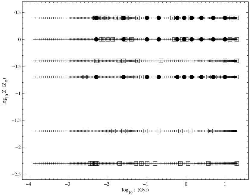
Figure 1: Distribution of the blindly-selected SSP spectra (denoted as “$\Box$”) employed for Ensemble Learning Component Independent Analysis in the age vs. metallicity space. The entire SSP spectra in the BC03 library (denoted as “+”) and the spectra used as templates by Tremonti et al. (2004, denoted as “$\bullet$”) are also shown for comparison.

Using evolutionary stellar population synthesis model, BC03 generated a high resolution library of synthetic galaxy spectra, GALAXEV , based on a new observed spectral library of stars, STELIB (Le Borgne et al. 2003). This library spans wide range of ages between $1\times 10^{5}$ and $2\times 10^{10}$ yr. The model spectra were calculated for 6 different metallicities (0.005, 0.02, 0.2, 0.4, 1.0 and 2.5 times of $Z\odot$) at a resolution of 3 Å FWHM across the wavelength range of $3200~{}-~{}9500$ Å (corresponding to a median resolving power $\lambda/\Delta\lambda\approx 2000$). The total number of the model spectra is 1326, 221 for each of the 6 metallicities (see Fig. 1 for the spectra distribution in the age/metallicity plane). Synthetic spectra with a larger wavelength range of $91~{}\AA~{}-160~{}\mu m$, at lower resolution are also computed.

3.1 EL-ICA of the SSP Spectra

In this subsection we apply the EL-ICA method to the high resolution SSP spectra in the GALAXEV. The 1326 SSP spectra are first truncated to wavelength range of $3322-9200$ Å  (the short wavelength limit is set by the high resolution wavelength range of the GALAXEV and the long wavelength limit is chosen to match that of the SDSS spectrograph) before further analyses. As a high-order statistical algorithm, EL-ICA converges very slow. In this paper, we only apply EL-ICA on a small subsample of the SSP spectra. 74 out of the 1326 SSP spectra are picked up as a subsample following the procedures below. First we select the eldest SSP spectrum (age = $2\times 10^{10}$ yr) with the highest metallicity ($5~{}Z\odot$, the upper right one in Figure 1) as a start point. In step 2 we move to the second highest metallicity ( $Z=Z\odot$): the 221 spectra are examined in the order of decreasing age, and the first one which is significantly different from the spectrum/spectra in the subsample is added to the subsample. The definition of “significantly different” is

$$\sqrt{\frac{1}{C}\sum_{k=1}^{C}\{\frac{[SSP^{i}(\lambda_{k})-SSP^{j}(\lambda_{k})]}{[SSP^{i}(\lambda_{k})+SSP^{j}(\lambda_{k})]/2}\}^{2}}~{}>~{}\frac{3}{50},$$ (2)

where C is the number of wavelength channels, and $\frac{3}{50}$ stands for 3 $\sigma$ significance level for the SSP spectra with standard S/N of $\sim 50$. Then we move to the next lower metallicity, and repeat the above selection. Once we reach the lowest metallicity, we turn over to the highest metallicity one, repeat the above steps, and so on. The subsample is selected to statistically represent the whole sample on the standard S/N level of $\sim 50$. The distribution of the derived subsample is displayed in Figure 1, where we can see that the 74 SSP spectra cover a wide range of age and metallicity. Note that there is no SSP younger than $\sim 2.5\times 10^{6}$ yr in our subsample. This is actually expected since that at $age\lesssim 10^{6}$ yr, the SSP are dominated by the hottest massive stars and the spectra are quite similar across the wavelength range of $3322-9200$ Å. We also plot in Figure 1 the age/metallicity coverage of a sample of stellar populations used by Tremonti et al. (2004). The main difference between the two is that our sample includes 6 metallicities while Tremonti et al.’s includes 3, and our sample is selected unsupervised.

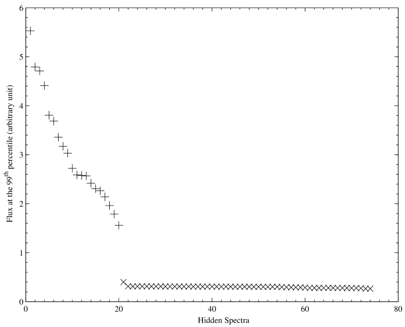
Figure 2: Distribution of the flux at the $99^{th}$ percentile of the 74 recovered Hidden Spectra. It is remarkable that flux of the first 20 Hidden Spectra (denoted as “+”) is much larger than that of the last 54 (denoted as “$\times$”s). The Hidden Spectra are sorted as descending of flux for visualization.

The EL-ICA method is applied to the 74 SSP spectra selected above, and 74 Hidden Spectra (HS) are derived. In Figure 2 we plot the flux at the $99^{th}$ percentile level for each of the 74 hidden spectrum. It is obvious that 54 of the hidden spectra have almost zero flux, comparing with the other 20. Then the first 20 HS are normalized at 5500 Å  and utilized to fit the 1,326 BC03 SSP spectra through linear least-squares fitting with non-negativity constraints,

$$SSP^{j}(\lambda)=\sum_{i=1}^{20}c^{j}_{~{}i}~{}HS^{i}(\lambda),~{}~{}c^{j}_{~{}i}\geq 0,~{}j=1,2,...,1326.$$ (3)

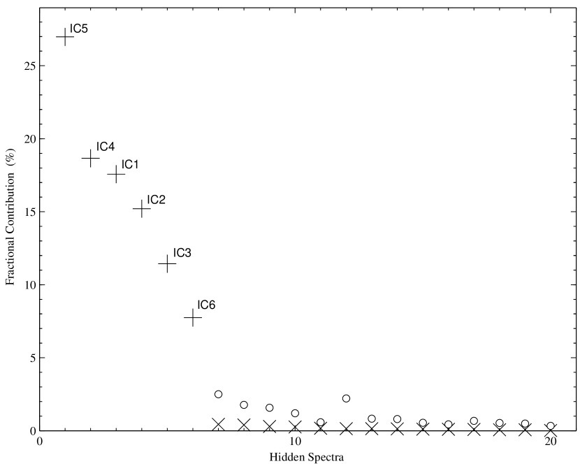
Figure 3: Distribution of the average fractional contribution of the 20 Hidden Spectra selected in Figure 2 to the 1,326 SSP spectra in the BC03 library. The Hidden Spectra are sorted as descending fractional contribution for clarity. It can be seen that the contribution of the first 6 Hidden Spectra (denoted as “+”) is significantly larger than that of the last 14 (denoted as “$\times$”). Even the largest fractional contribution of the last 14 Hidden Spectra to the individual SSP spectrum (denoted as “$\circ$”) is $<2.5\%$, and their cumulative contribution is $\simeq 2.4\%$. The 6 ICs are named in the order of their “spectral types” (see the text and Figure 4).

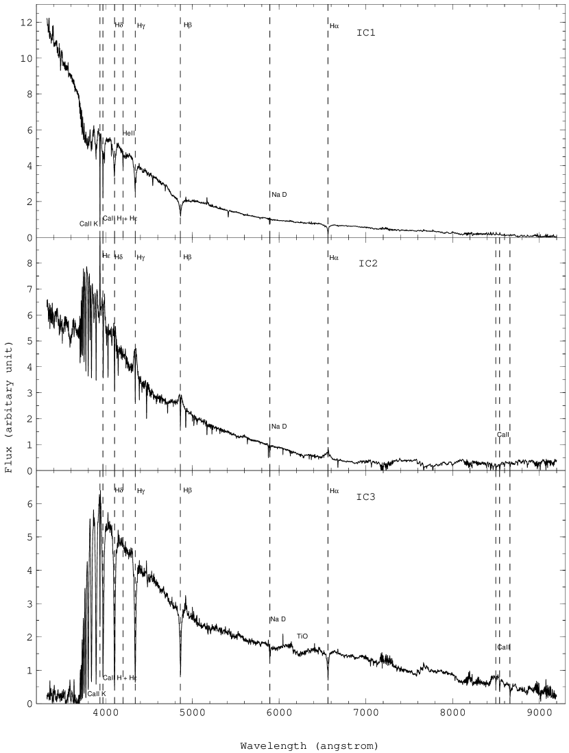
Figure 4: The spectra of the 6 ICs ordered by their “spectral types” (from “early” to “late”, see detailed description in the text). The prominent spectral features are labelled.

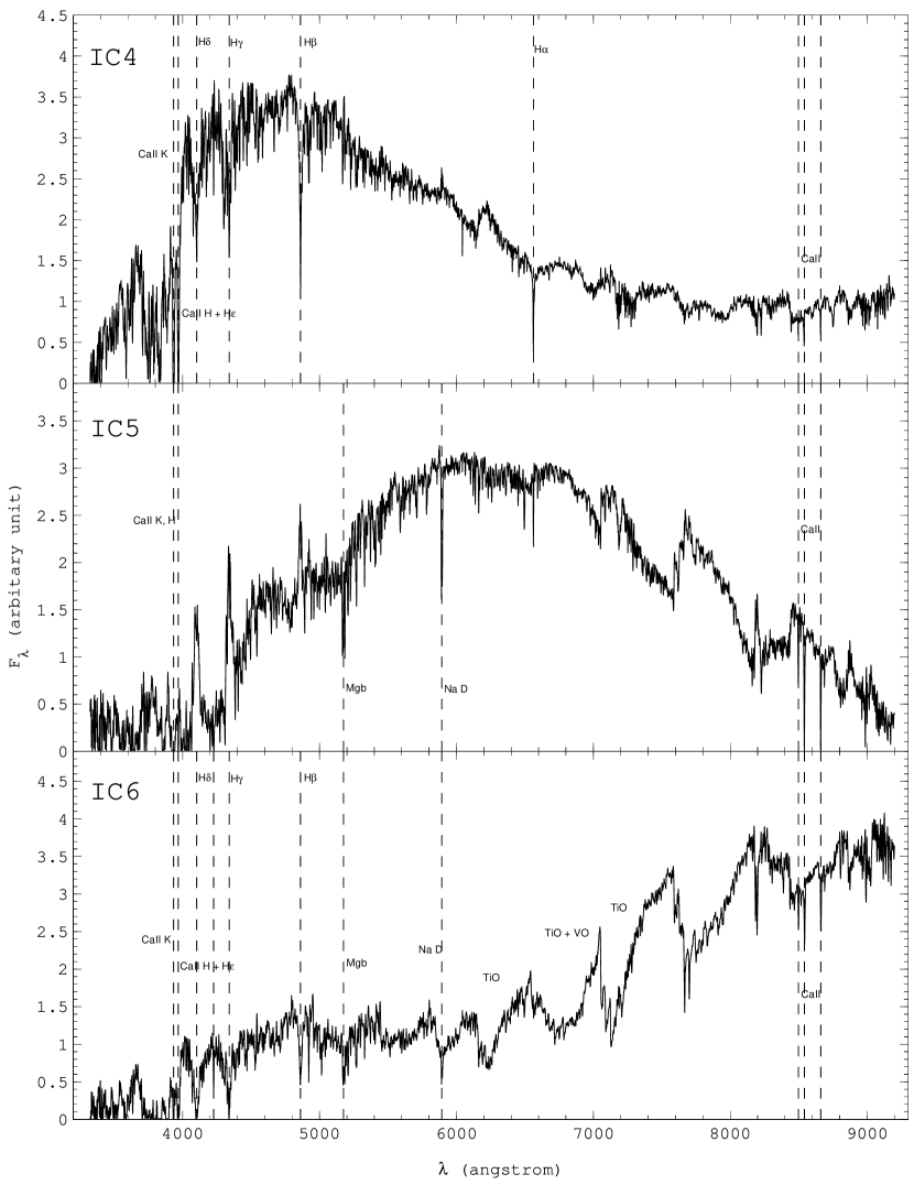
Figure 4: Continued…

We define the fractional contribution of the $i^{th}$ HS to the $j^{th}$ SSP as the normalized best fitting coefficient, $c^{j}_{~{}i,norm}=\frac{c^{j}_{~{}i}}{\sum_{i=1}^{20}c^{j}_{~{}i}}\times 100\%$, and the average fractional contribution of the $i^{th}$ HS to the BC03 SSP, $c_{i}=\frac{\sum_{j=1}^{1326}c^{j}_{~{}i,norm}}{1326}$. The distribution of the average fractional contribution of the 20 HS is shown in Figure 3. It can be seen that the contribution of the first 6 HS is significantly larger than that of the rest ones. The accumulative contribution of the first 6 HS amounts to $\sim 97.6\%$, and that of the last 14 HS is only $\sim 2.4\%$. We obtain similar results while fitting the spectra of the SDSS galaxies with the 20 HS (see §4). The 6 hidden spectra are therefor chosen as the final Independent Components (ICs), the spectra of which are presented in Figure 4. Actually none of the contribution of the last 14 HS to the individual SSP spectrum is larger than $2.5\%$.

3.2 Interpretation of the IC Spectra

Though EL-ICA, we compressed the 1326 BC03 SSP spectra into 6 non-negative ICs. The physical meaning of the 6 ICs is interesting and could be easily understood through examining the spectra visually. The 6 ICs are named in the order of the spectral type (“early—late”).

IC1

represents the blue continuum of O star. However, the CaII H and K lines at 3933 and 3968 Å, which are stronger in late-type stars than in early-type stars, also exist;

IC2

is similar to the spectrum of B star. Nevertheless, the absorption lines of neutral metals and molecules such as TiO and titanium Oxide, which are normal in spectra of later than K stars, are also identified;

IC3

shows extremely strong Balmer absorption lines and Balmer jump in the blue part of the spectra, even more prominent than A stars. But the Ca II triplet at 8498, 8542, and 8662 Å, and more lines of neutral metals and molecules appear in the red;

IC4  and IC5

are somewhat like hybrids of F to K stars, with stronger neutral metal and molecule lines.

IC6

is similar to the spectrum of M star in the long wavelength range but shows high order Balmer absorption lines in the short wavelength.

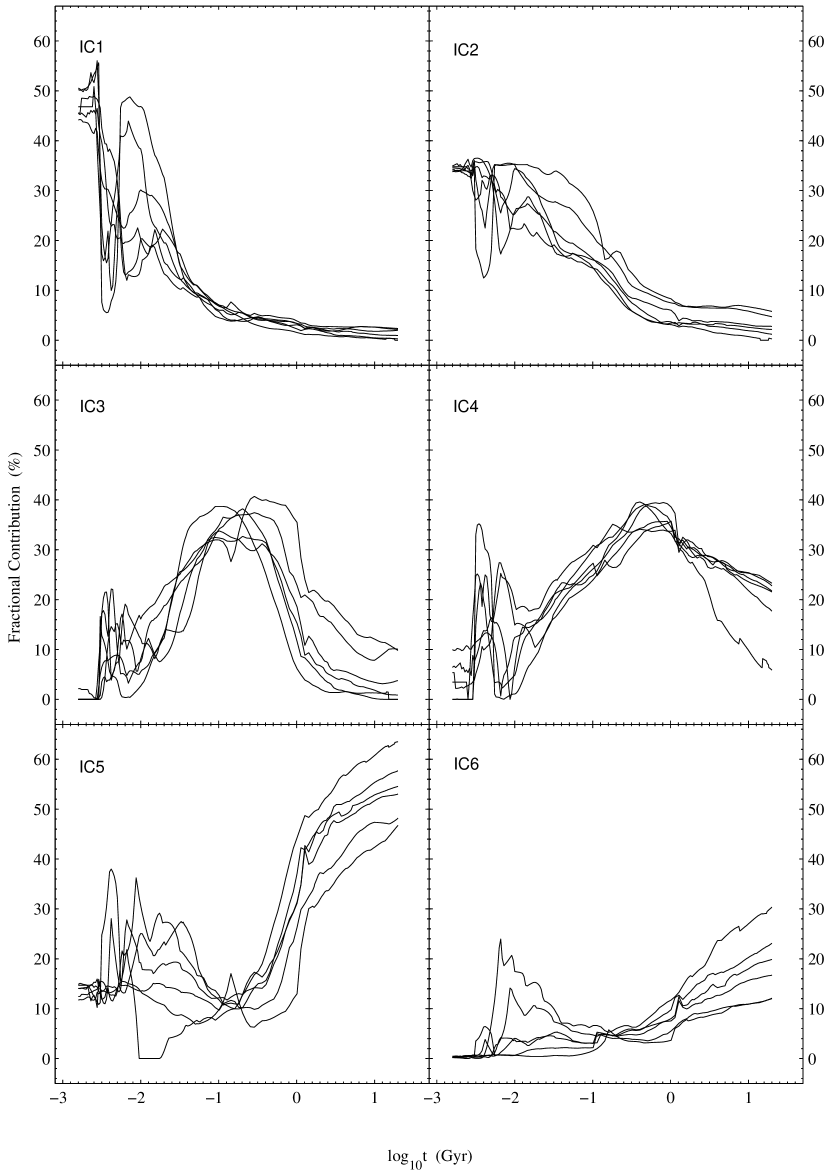
Figure 5: The projection of the SSP spectra on the $ICi^{th}$ versus age. Each line denotes one metallicity.

The spectral properties of the ICs imply that a tight correlation between the stellar population age and the ICs. In Figure 5 we plot the contribution of 6 ICs to individual SSP spectrum as a function of age for 6 metallicities, where clear correlations between the contributions of ICs and the age can be seen. For instance, the fractional contribution of $IC1\gtrsim 8\%$ indicates an age of $t\lesssim 10^{8}$ yr, and $IC3\gtrsim 30\%$ indicates $10^{8}\lesssim t\lesssim 10^{9}$, corresponding the age of the so-called “E+A” galaxies (e.g., Dressler & Gunn 1983).

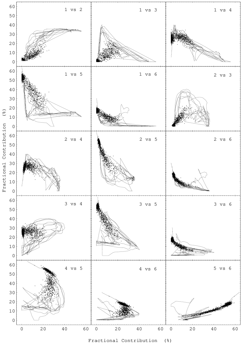
Figure 6: The projection of the SSP (lines) and the SDSS galaxy spectra (dots) on the IC (x-axis) vs IC (y-axis) plane. The $\sim 1,000$ high spectral quality galaxies are randomly selected from the SDSS DR2.

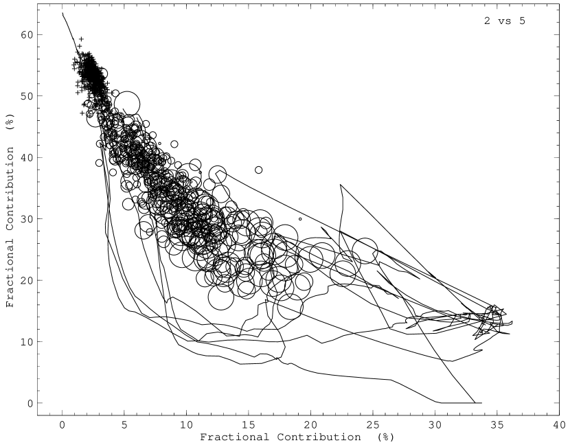
Figure 7: A close look at the center penal of Figure 6 (IC2 (x-axis) vs IC5 (y-axis)), but with the SDSS absorption line galaxies denoted as cross and emission line galaxies denoted as circle of size increasing with the equivalent width of $H\alpha$, $EW(H\alpha)$. It is obvious that the emission line galaxies are well separated from absorption line galaxies in this diagram. Also note that galaxies with larger contribution of IC2, corresponding to young populations, tend to have stronger emission lines.

According the EL-ICA model, a spectrum of a stellar system corresponds to a vector in the 6-D IC space. In Figure 6 we plot the projection of the SSP spectra on the IC versus IC planes to give a visual impression of the distribution of stellar systems in the 6-D IC space. One of these diagrams, IC2 versus IC5, is zoomed to highlight the detailed features in Figure 7. The evolutionary track of an SSP in the IC space, though very complex, is treatable, because the spectra of a specific Simple Stellar Population, $SSP^{j}$, is determined by its age, t, and metallicity, Z, in the frame work of the BC03’s model; and in the same time it can be expressed as a non-negative linear combination of the 6 ICs,

$$SSP^{j}(\lambda)=SSP^{j}(t,Z)=\sum_{i=1}^{6}c^{j}_{~{}i}~{}IC^{i}(\lambda).$$ (4)

In principle, the correspondence of age and metallicity, (t,Z), and a 6-dimension array of the 6-IC expanded coefficients, ($c^{j}_{~{}i},~{}i=1,2,...6$), can be found.

The spectrum of any stellar system, e.g., a star cluster or a galaxy (with no extinction and stellar velocity dispersion), can also be expressed as a non-negative linear combination of the 6 ICs,

$$g(\lambda)=\sum_{i=1}^{6}g_{i}~{}IC^{i}(\lambda).$$ (5)

Thus any stellar system can be decomposed into $N_{*}$ SSPs of different ages and metallicities,

$$g(\lambda)=\sum_{j=1}^{N_{*}}s_{j}~{}SSP^{j}(\lambda)$$ (6)

where the minimum number of SSP required is $N_{*}\leq 6$. The coefficients, $s_{j}$ can be determined by solving the following 6 simultaneous linear equations,

$$g_{i}=\sum_{j=1}^{N_{*}}s_{j}c^{j}_{~{}i},~{}~{}(N_{*}\leq 6,~{}i=1,2,...,6).$$ (7)

Note in most cases, the solutions are not unique. We adopt the following strategy to choose the closest solutions: The $1^{st}$ SSP is chosen from the 74 SSPs described in §3.2 by minimizing the Euclidean distance in the 6-D IC space between the SSP and the galaxy under study. Then the $2^{nd}$ SSP is picked to further reduce the distance. This procedure is repeated until the improvement is no longer significant. For a majority of the galaxies, $N_{*}=2-6$ SSPs are needed to reconstruct the original spectra. The reliability of this solution is tested in §5.

4 Modelling the SDSS Galaxies

In this section we use the 6 ICs to model the SDSS spectra, which have comparable spectra resolution with that of GALAXEV. The spectra of $\sim 2.6\times 10^{5}$ galaxies in the SDSS DR2 (Abazajian et al. 2004) are fitted to exploit their spectral features, and in the meantime to test our new technique.

4.1 Fitting the Galaxy Spectra

The $\sim 2.6\times 10^{5}$ galaxies are corrected for the foreground galactic extinction in the first place using the extinction curve of Schlegel et al. (1998) and transformed to their rest frame using the redshift provided by the SDSS spectroscopic pipeline (Schneider et al. 2002). The derived galaxy spectra can be fitted by the 6 ICs as:

$$g^{obs}(\lambda)=A(E_{B-V},\lambda)\sum_{i=1}^{6}g_{i}~{}IC^{i}(\lambda,\sigma_{*}),$$ (8)

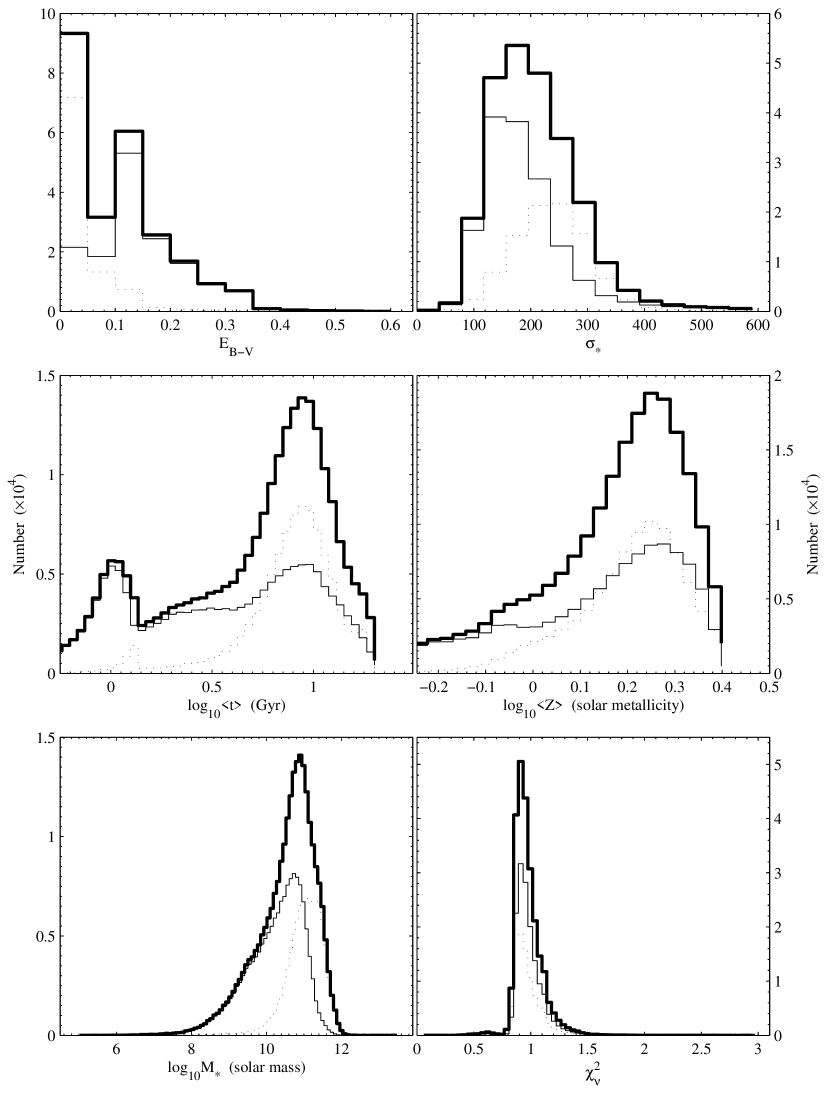
Figure 8: The distribution of starlight reddening ($E_{B-V}$, upper left panel), stellar velocity dispersion ($\sigma_{*}$, upper right panel), light-weighted average age ($<t>$, middle left panel), light-weighted average metallicity ($<Z>$, middle right panel), stellar mass ($M_{*}$, lower left panel), and reduced $\chi^{2}$ ($\chi^{2}_{\nu}=\chi^{2}/d.o.f$, lower right panel) for model fits of all the $\sim 2.6\times 10^{5}$ galaxies in the SDSS DR2. Total objects are denoted as thick solid lines, absorption line galaxies as dot lines, and emission-line galaxies, including HII galaxies, AGN and composite objects as thin solid lines. Aperture effect is not corrected.

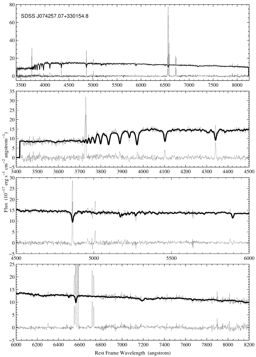
Figure 9: Examples of nonnegative linear least-square fits of the galaxy spectra in the SDSS DR2. The fits are yielded using the 6 ICs derived through the EL-ICA method. Emission lines, when present, are filtered to perform the fit. The upper panel displays the model fit as a whole and detailed features are highlighted in the lower three panels. In each panel, the upper two lines denote the observed spectrum (thin curves) and the modelled spectrum (thick curves). The lower thin line denotes the residual (or pure emission line) spectrum. The apparent mismatch around 6900 Å  is due to the residual telluric absorption in the spectra of the BC03 SSPs, which we use to derive the templates.

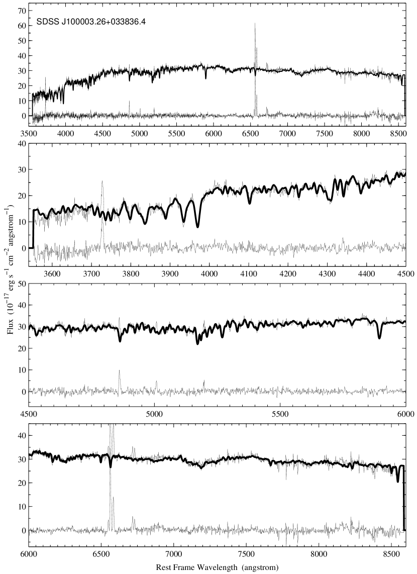
Figure 9: Continue…

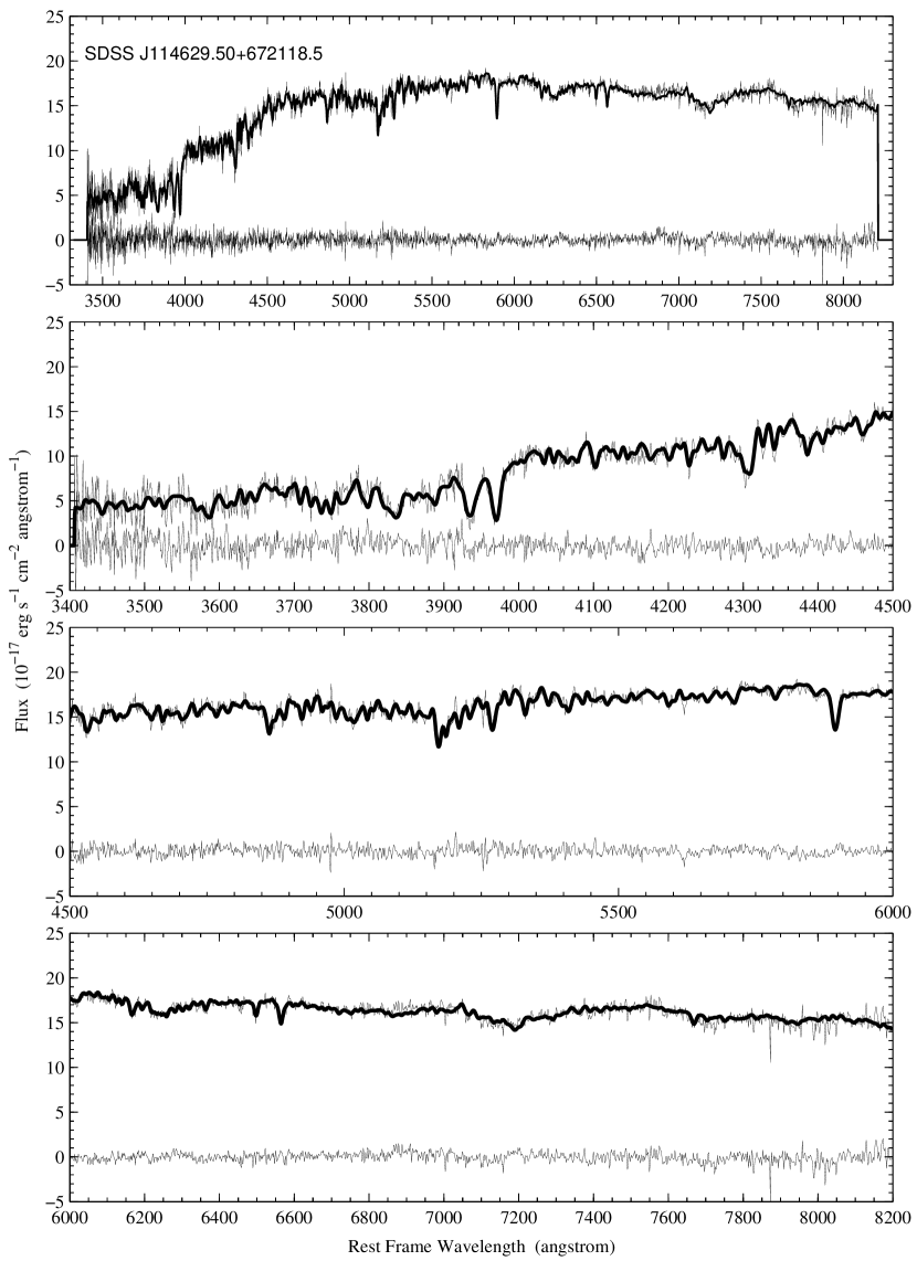
Figure 9: Continue…

where $g^{obs}(\lambda)$ is the observed spectrum of the galaxy under study, $IC^{i}(\lambda,\sigma_{*})$ is the $i^{th}$ IC broadened by convolving with a Gaussian of $\sigma_{*}$ width to match the stellar velocity dispersion of the galaxy, and $A(E_{B-V},\lambda)$ is the intrinsic starlight reddening (an SMC-like extinction curve is assumed, Pei 1992). The final fit is done through minimizing reduced $\chi^{2}$, and $E_{B-V}$, $\sigma_{*}$, and $g_{i}$ (i=1, 2, …, 6) are non-negative free parameters. During the fit, the prominent emission lines (Balmer systems, $H_{n<6}$ and strong forbidden lines such as $[OII]\lambda 3727$, $[OIII]\lambda\lambda 4959,5007$, $[OI]\lambda 6300$, $[NII]\lambda\lambda 6548,6583$ and $[SII]\lambda\lambda 6716,6731$) are masked out through excluding the wavelength region (5 Å  in width) for each line. Note if there exists nuclei emission ($\sim 1,200$ objects in the “galaxy” catalog of the SDSS DR2), an additional power law and broader emission line components are added to the fit. Bad pixels in the spectra flagged by the SDSS pipeline are also excluded. We then subtract the modelled stellar spectrum and fit emission line with various Gaussians (Dong et al. 2005). Replacing the masked emission line ranges with the line fitting results, we reiterate the above procedures until both the fitting of stellar spectrum and emission lines are acceptable. For most of the spectra ($\gtrsim 95\%$), two iterations are enough. In Figure 8 (lower right panel) we present the reduced $\chi^{2}/d.o.f$. The fits are incredibly good for most of the spectra, with only $\sim 2\%$ having $\chi^{2}/d.o.f$ $>$ 1.5. Representative example of the fit are displayed in Figure 9.

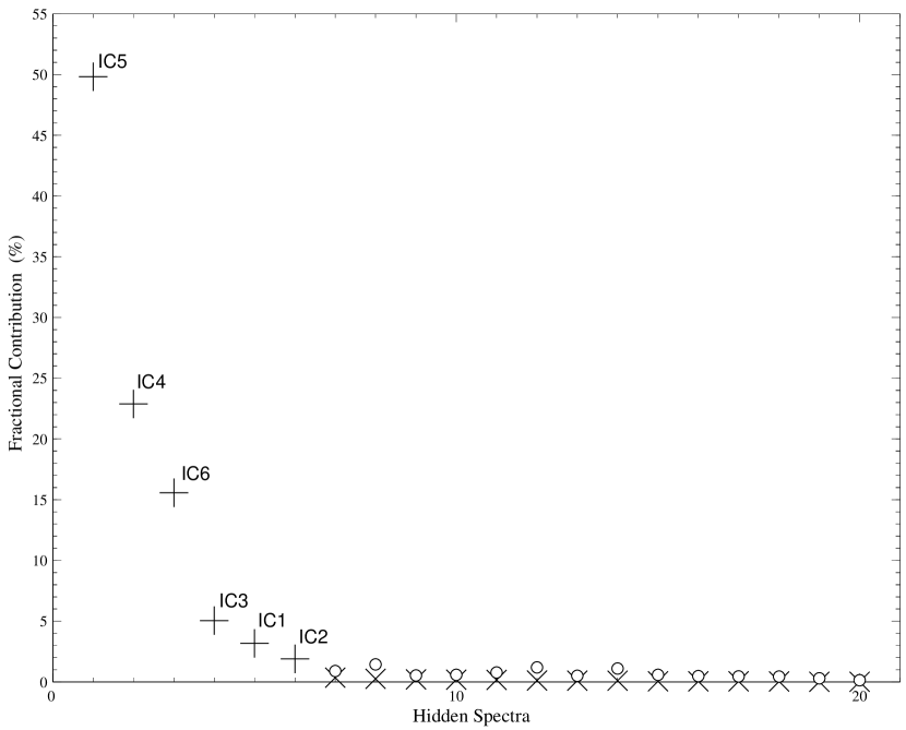
Figure 10: Same as Figure 3 but for $\sim 10^{4}$ high quality spectra of the SDSS galaxies. The total contribution of the 6 ICs (the first 6 Hidden Spectra) is $98.36\%$, which is even higher than their total contribution to the BC03 SSP spectra. The ICs are ordered by their spectral types, as in Figure 3 and 4.

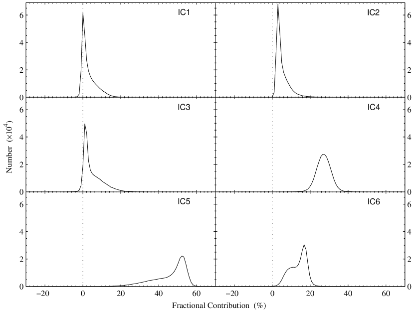
Figure 11: Distribution of fractional contribution of the 6 ICs to the $\sim 2.6\times 10^{5}$ galaxies in the SDSS DR2, if releasing the non-negative requirement. It is remarkable that only a majority of the contribution is non-negative and the amplitude of negative contribution is negligible.

For about ten thousand high quality SDSS spectra, we repeat our fit using the 20 HS described in §3. The average contribution of each HS is plotted in Figure 10, which is similar to that of Figure 3. This further confirms that the 6 ICs we identified are representative enough to embody almost all of the information in the spectra of any stellar system. Finally we try a linear least-square fit to all of the $\sim 2.6\times 10^{5}$ SDSS galaxies using the 6 ICs with non-negative constraint released. The contributions of the 6 ICs to each spectrum is shown in Figure 11. It is remarkable that, even without the non-negative restriction, $\sim 96.2\%$ of the coefficients are non-negative and $\gtrsim 99.9\%$ of the negative contribution is $\lesssim 2.5\%~{}$.

4.2 Results

The following spectral parameters of galaxies are derived:

Starlight Reddening

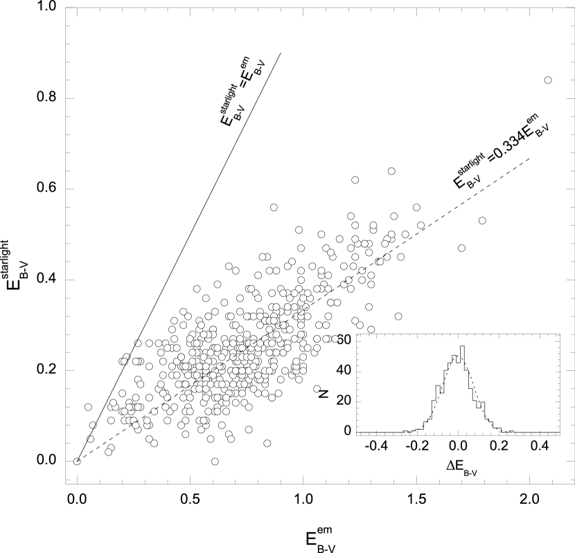
Figure 12: Mean color excess of starlight, $E_{B-V}^{starlight}$, obtained by our continuum model fitting versus that of emission lines, $E_{B-V}^{em}$, estimated by Balmer decrement, $H\alpha/H\beta$, for $\sim 500$ HII galaxies with high quality spectra (median S/N ratio $\gtrsim 30$ and $H\beta$ flux $>10~{}\sigma$) arbitrarily selected from the SDSS DR2. $E_{B-V}^{em}$ is estimated assuming an intrinsic Balmer decrement, $H\alpha/H\beta=2.87$ and the SMC extinction curve. The dash line is best linear fitting. The inset plot shows the deviation of the measured values and the best fit line, $\Delta E_{B-V}=E_{B-V}^{predicted}-E_{B-V}^{measured}$. The dashed line is Gaussian with $\sigma=0.076~{}mag$.

Light from Galaxies suffers from various intrinsic reddening due to different amount of dust. By fitting the optical spectra, we found that in more than half of the SDSS galaxies, the color excess of starlight is $\gtrsim 0.1~{}mag$ (Figure 8, upper left panel). This indicates that reddening must be properly taken into account while trying to extract the stellar mass and Star Formation Rate (SFR) from galaxy spectra. In Figure 12 we plot starlight extinction obtained using the method presented in this paper and that estimated according to Balmer decrement, $H\alpha/H\beta$. It can be seen that starlight extinction is well correlated with the extinction of nebular emission lines, suggesting the starlight reddening obtained using EL-ICA method is reasonable. A best linear fitting reveals $E^{starlight}_{B-V}=(0.334\pm 0.01)E^{em}_{B-V}$. This slope is much flatter than that of Calzetti et al. (1994), who obtained a value of 0.5.

Stellar Velocity Dispersion

Similar to Li et al. (2004), stellar velocity dispersion, $\sigma_{*}$, can be given directly by the fit (Figure 8, upper right panel). The results from two methods are consistent.

Stellar Population and Metallicity

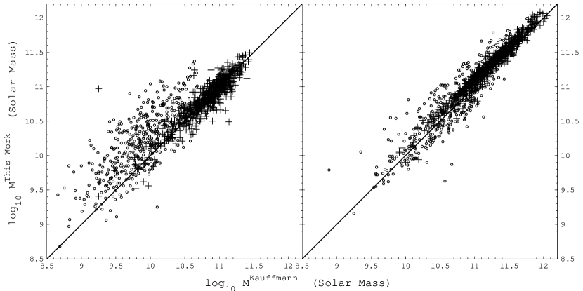
Figure 13: Our measurement of stellar mass compared with that of Kauffmann et al. (2003). Only $\sim 1,000$ typical SDSS galaxies are shown for clarity. Emission line galaxies are denoted as circle and absorption line galaxies as cross. In the left panel, stellar mass of our measurement is corrected for intrinsic extinction but not for aperture effect, and value of Kauffmann et al. was not corrected for both of dust reddening and aperture effect. Stellar mass is corrected for both of aperture effect and dust reddening in the right panel. Our measurement agrees well with Kauffmann et al. The agreement is better for absorption line galaxies than for emission line galaxies, in which dust reddening is often more serious.

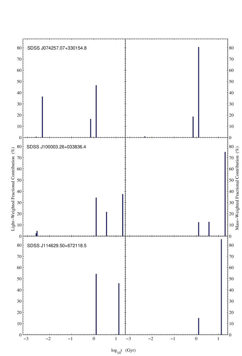
Figure 14: The modelled star formation histories of the 3 SDSS galaxies as in Figure 9, expressed as light (left panels) and mass (right panels) fractions versus ages.

Another advantage of the EL-ICA method over PCA-based approach is that light/mass-weighted ages, metallicities, and stellar mass can be derived from integrated galaxy spectra, since the galaxy spectrum is non-negative combination of the spectra of 6 ICs or $N_{*}\leq 6$ SSPs. The results are also displayed in Figure 8. Our measurement of stellar mass is compared with that of Kauffmann et al. (2003) in Figure 13. In fact, stellar population can be revealed with higher resolution than mere average age. Figure 14 shows the modelled star formation histories of the same 3 SDSS galaxies displayed in Figure 9, expressed as light and mass fractions versus age. Furthermore, as the recovered number of ICs, in turn the number of the SSPs needed to model the spectrum of a galaxy, is no more than six, the probability of over-fit can be greatly reduced.

It is interesting to inspect the distribution of the observed galaxy spectra in the IC space. We randomly select $\sim 1,000$ galaxies with median $S/N\gtrsim 30$ from the SDSS DR2 and plot them in Figure 6 and 7. Most of the galaxies are enveloped by the SSPs. This is consistent with the assumption that the star formation histories of any galaxy can be expressed as a sum of discrete bursts. Absorption-line galaxies tend to distribute in the surface of the envelop formed by the SSPs, and they are well separated from emission-line galaxies. This is because absorption-line galaxies are passively evolving ones, which only contain old and/or middle-aged SSP(s), while emission-line (star-forming) galaxies in the local universe often comprise both young and old stellar populations. We note that galaxies with larger contribution of “early-type” ICs, corresponding to young populations, tend to have stronger emission lines. This indicates that, 1) spectral classification of galaxies can be made using the EL-ICA method; and 2) the optical stellar spectrum of a galaxy can serve as a star formation rate indicator. Using the $N_{*}\leq 6$ recovered SSP spectra, the near-IR SED can also be estimated by extrapolating from the optical data. We leave this issue for future studies.

5 Reliability of the Derived Parameters

We perform extensive tests to estimate the reliability of the parameters yielded by our galaxy spectra modelling. For this purpose, 59400 synthetic galaxy spectra are created from the library of the BC03 SSP following the steps below:

• We first pick up 60 SSP spectra, with 10 different ages (0.005, 0.01, 0.02, 0.06, 0.2, 0.6, 1.4, 5, 10, 15 Gyr) for each of the 6 metallicities.

• 6 out of the 60 SSP spectra are randomly selected, one for each metallicity. The 6 spectra are then normalized at 5500 Å and combined with random weights to create one synthetic spectrum. The total weight of the 6 SSPs is normalized to 1. Repeating this step we get a total of 60 synthetic spectra.

• The 60 spectra are then broadened by convolving with Gaussian function with stellar velocity dispersion of $\sigma_{*}=30m~{}km~{}s^{-1}$, m=1, 3, …, 15.

• Different reddening are applied to enlarge the sample to 9,900 spectra, with $E_{B-V}=0.1n~{}mag$ , n=0, 1, …, 11.

• Gaussian noise is finally added to yield spectra sets with S/N=10, 15, 20, 30, 40, 50 respectively.

In this way 59,400 synthetic galaxy spectra are created, with wide coverage of ages and metallicities, 15 stellar velocity dispersions, 11 color excess, and 6 S/N levels. The synthetic galaxy spectra in the wavelength range of $3322-9200$ Å are fitted using Equation 8 as we model the galaxies in the SDSS DR2 and the input parameters are recovered simultaneously. During the fit, we mask the same potential emission line regions used to fit the real galaxies, although it is not required because the synthetic spectra do not contain emission lines. This makes our test results directly comparable to the results from the real spectra:

Starlight Reddening

There is no systematic discrepancy between the recovered and the input starlight reddening. In Figure 15, we plot the rms of the measured color excess. The uncertainty is not sensitive to the S/N ratio of synthetic galaxy spectra, provided $S/N\gtrsim 15$ per pixel. This is understandable because S/N ratio does not significantly affect the SED.

Stellar Velocity Dispersion

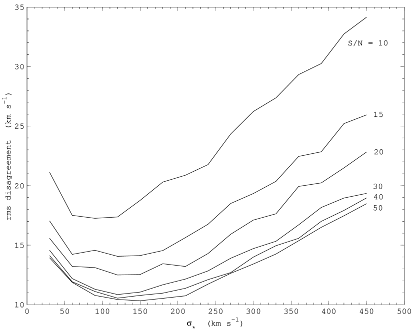
Figure 16: The uncertainty (rms) of the measured stellar velocity dispersion for the artificial spectra with different signal-to-noise ratios.

The recovered and the input stellar velocity dispersion, $\sigma_{*}$, are plotted in Figure 16. The disagreement between the two is $\lesssim 30~{}km~{}s^{-1}$ for $S/N>10$ and the measurement uncertainty decreases rapidly with increasing S/N ratio. For typical spectral quality of the SDSS galaxies ($S/N\sim 20$), $1~{}\sigma$ error is $\lesssim 20~{}km~{}s^{-1}$.

Stellar Populations, Metallicities and stellar mass

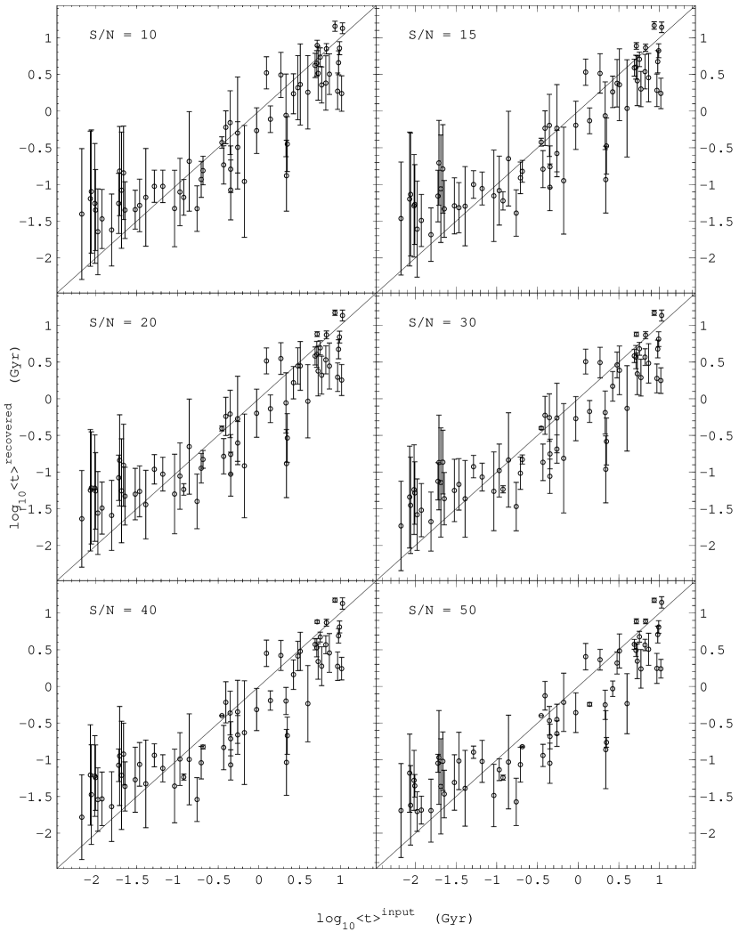
Figure 17: Comparison of the recovered and input light-weighted average age. The error bar denotes $1~{}\sigma$ rms of the recovered light-weighted average age.

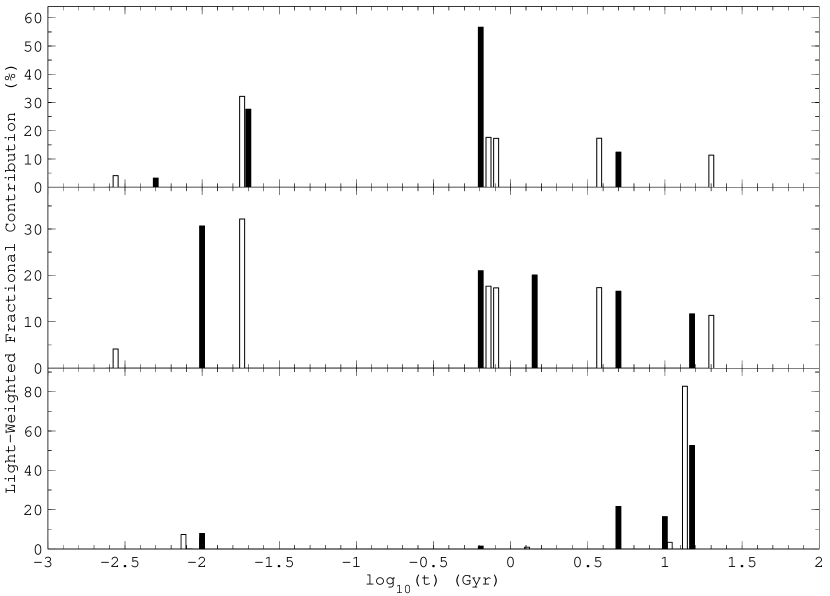
Figure 20: Comparison of the recovered (hollow) and input (filled) star formation histories of 3 randomly selected synthesized galaxies.

Using the EL-ICA method, one can decompose a galaxy spectrum into $N_{*}\leq 6$ SSPs of different ages and metallicities. In turn, stellar mass, light (or mass)-weighted average age and metallicity can be derived. The comparisons between the recovered and input values are displayed in Figure 17-19. The results indicate that the age-metallicity degeneracy can at least be partly broken and star formation histories be estimated. Figure 20 shows that the star formation history can be resolved with higher resolution than average age. It can be seen that, though the star formation histories of a galaxy cannot be exactly recovered due to the age-metallicity degeneracy, they can be estimated with meaningful accuracy.

6 Comparison with PCA

PCA is a classic technique in statistical data analysis, feature extraction, and data compression. It has been successfully used in studies of the multivariate distribution of astronomical data (e.g., Efstathiou & Fall 1984; Connolly et al. 1995; Folkes et al. 1996; Glazebrook et al. 1998; Bromley et al. 1998; Folkes et al. 1999; Madgwick et al. 2002; Li et al. 2005). Given a set of multivariate observations, the basic PCA problem is to find a small set of variables with less redundancy that can give as good representation as possible. Though the goal of PCA is similar to that of ICA, the method used to get rid of redundancy is different: In PCA the redundancy is measured by correlations between observed data, while the much richer concept of independence is used in ICA. The advantage of ICA has been mentioned in §2.1. However, using only the correlations in PCA has likewise its advantage that the analysis can be based on 2nd-order statistics only. It would be interesting to make comparison between the two techniques. In this section, we apply PCA to analyze the same data set as we have done in the previous sections using ICA.

We first apply PCA to the truncated SSP spectra in GALAXEV mentioned in §3.1, which are also normalized at 5500 Å. All of the 1326 spectra in the library, instead of a subsample, are analyzed this time since PCA converges much faster than EL-ICA. We subtract the mean from the spectra before PCA as Madgwick et al. (2002) and adopted the mathematical formulation of PCA given in Folkes et al. (1999). The PCA analysis generates a set of eigenspectra, which are denote as $PC^{i}(\lambda)$ (i=1,2,3,…, ordered by their relative importance measured as variance), with the main spectral features of the whole library concentrated in the first few. Indeed, we find that the cumulative contribution of the first three PCs to the total variance amounts to 99.7%, and the significance of each successive PC drops off sharply. We determined the number of PCs required to represent GALAXEV as follows. Initially, the SSP spectra in GALAXEV were fitted by the first three PCs as Equation 4 substituting PCs to ICs and releasing the non-negative restriction on $c^{j}_{~{}i}$. By adding successively the next PC to the model, we calculate the significance of the improvement to the fit using the F-test,

$$\alpha_{F} = \int_{F}^{\infty}dFp(F|\Delta P,N-P_{1})=I_{\frac{N-P_{1}}{N-P_{1}+\Delta P\cdot F}}\big{(}\frac{N-P_{1}}{2},\frac{\Delta P}{2}\big{)},$$ (9)

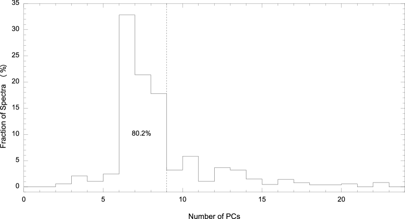
Figure 21: Histogram of the F-test to determine the number of PCs enough to represent GALXEV.

where, the $F$-statistics $F=\frac{\Delta\chi^{2}/\Delta P}{\chi_{1}^{2}/(N-P_{1})}$, $P_{1}$ and $\Delta P=1$ are the numbers of thawed parameters of the previous model and of the additional freely varying parameters in the current model, $I$ the incomplete beta function. Adopting a critical significance of $\alpha_{F}=0.05$, we find that more than 80% SSP spectra can be well-fitted using the first 9 PCs (see Figure. 21), which are then chosen as our final spectral templates (also denoted as PCs).

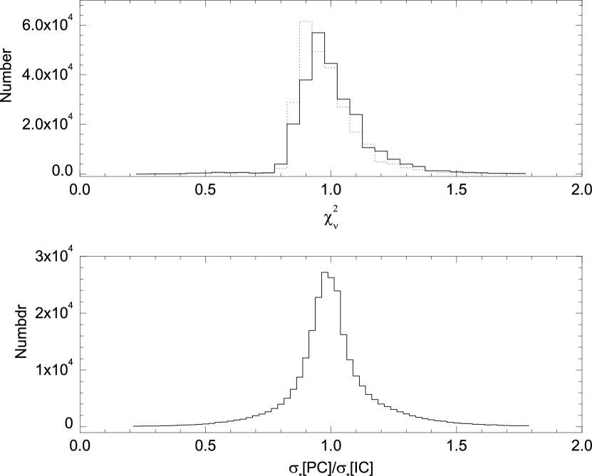
Figure 22: The upper panel shows the distribution of reduced $\chi^{2}$ for PCA model fits of all the $\sim 2.6\times 10^{5}$ galaxies in the SDSS DR2 (solid line) compared with EL-ICA model (dotted line). Stellar velocity dispersion obtained using the PCA model $\sigma_{*}[PC]$ and EL-ICA model $\sigma_{*}[IC]$ is compared in the lower panel.

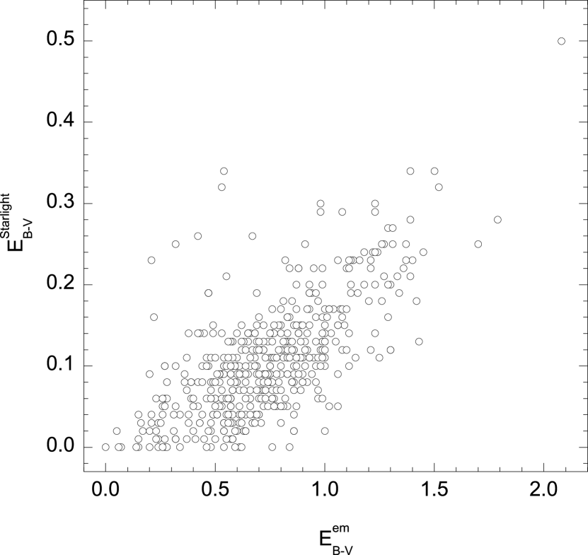
Figure 23: Same as Figure 12 but the starlight reddening is derived using PCA method.

Then we fit all the galaxies in the SDSS DR2 using Equation 8 in the same way as described in §4.1, substituting the nine PCs to the six ICs and releasing the non-negative restriction on $g_{i}$. It can be seen from Figure 22 (upper panel) that the distribution of reduced $\chi^{2}$ is similar to that of EL-ICA models, indicating that starlight in observed galaxy spectra can also be well reproduced using the nine PCs. Like EL-ICA method, we can also obtain stellar velocity dispersion as a by-product. We compare the measured values of $\sigma_{*}$ using the two methods and find that they agree with one another with in the measurement uncertainty (Figure 22, lower panel). We plot in Figure 23 the starlight extinction as determined by PCA method against the extinction of nebular emission lines for the same $\sim 500$ HII galaxies as in §4.2. The two values are also correlated but the scatter is a little larger than Figure 12. This result is consistent with that of Li et al. (2005). These authors also tried to determine starlight reddening using PCA based approach and found the typical uncertainty is $\sim 0.2~{}mag$, much larger than that yielded by the EL-ICA method ($\sim 0.06~{}mag$, see §5.1). Due to the fact that we cannot force PC spectra non-negative (they must be perpendicular with one another) and the combination coefficients, we are unable to obtain the stellar contents of galaxies.

7 Summary

We employ EL-ICA to analyze stellar system spectra and compress the BC03 stellar spectral library into 6 non-negative ICs. In consequence, the spectrum of a stellar system can be compressed to a vector in the 6-dimension space spanned by the 6 ICs, which redescribes the original data in a very condense form. These 6 ICs are used as templates to model the spectra of normal galaxies in the SDSS DR2. Important spectral parameters, such as starlight reddening, stellar velocity dispersion, stellar contents and star formation histories, can be obtained simultaneously. Extensive tests show that satisfactory accuracy can be achieved to these parameters for the typical spectral quality of the SDSS. The ICA model does not depend on previous knowledge. Using the EL algorithm to ICA model, we can also force the ICs and the combination coefficients non-negative and find the simplest interpretation of the observed galaxy spectra. The physical meaning of the ICs and the separation of the observed galaxy spectra can be easily understood. All the features of stellar spectrum are taken into account in the fit, hence the conundrum of over-fit is greatly mitigated. The method presented in this paper open a new way to model galaxy spectra. Its robustness and high efficiency make it applicable to extract the spectral characteristics of galaxies observed by modern large sky area surveys.

Figure 15: The uncertainty (rms) of the measured starlight extinction for the artificial spectra with different signal-to-noise ratios.

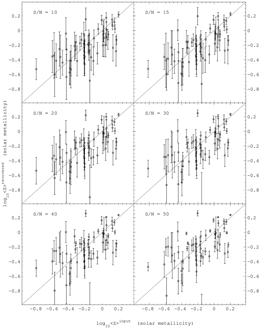
Figure 18: Comparison of the recovered and input light-weighted metallicity.

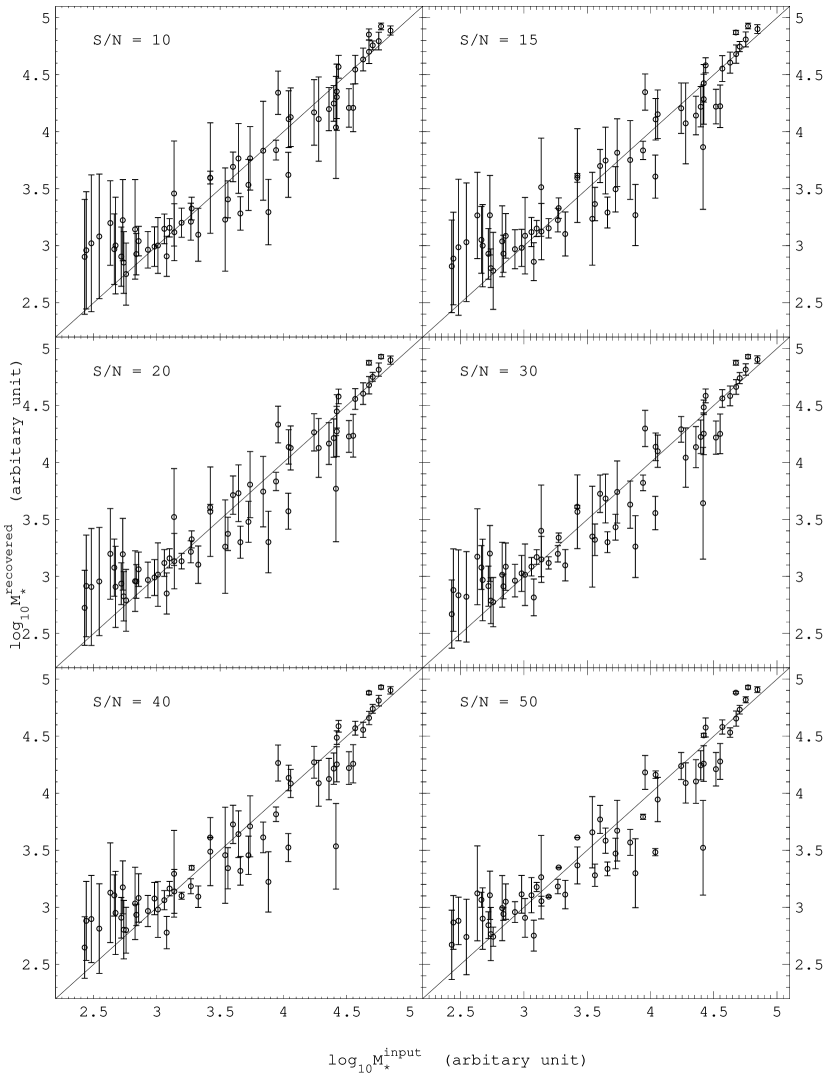
Figure 19: Comparison of the recovered and input stellar mass.

References

- Abazajian et al. (2004) Abazajian, K., et al. 2004, AJ, 128, 502
- Baccigalupi et al. (2000) Baccigalupi, C., et al. 2000, MNRAS, 318, 769
- Bromley et al. (1998) Bromley, B. C., Press, W. H., Lin, H., & Kirshner, R. P. 1998, ApJ, 505, 25
- Bruzual & Charlot (2003) Bruzual, G. & Charlot, S. 2003, MNRAS, 344, 1000, BC03
- Calzetti, Kinney, & Storchi-Bergmann (1994) Calzetti, D., Kinney, A. L., & Storchi-Bergmann, T. 1994, ApJ, 429, 582
- Charbonnel et al. (1999) Charbonnel, C., Däppen, W., Schaerer, D., Bernasconi, P. A., Maeder, A., Meynet, G., & Mowlavi, N. 1999, A&AS, 135, 405
- Chu & Zhao (1998) Chu, Y. & Zhao, Y.-H. 1998, IAU Symp. 179: New Horizons from Multi-Wavelength Sky Surveys, 179, 131
- Cid Fernandes, Sodré, Schmitt, & Leão (2001) Cid Fernandes, R., Sodré, L., Schmitt, H. R., & Leão, J. R. S. 2001, MNRAS, 325, 60
- Connolly et al. (1995) Connolly, A. J., Szalay, A. S., Bershady, M. A., Kinney, A. L., & Calzetti, D. 1995, AJ, 110, 1071
- Dong et al. (2004) Dong, X., Zhou, H., Wang, T., Li, C., & Zhou, Y. 2005, ApJ, in press
- Dressler & Gunn (1983) Dressler, A. & Gunn, J. E. 1983, ApJ, 270, 7
- Efstathiou & Fall (1984) Efstathiou, G., & Fall, S. M. 1984, MNRAS, 206, 453
- Filippenko & Sargent (1988) Filippenko, A. V. & Sargent, W. L. W. 1988, ApJ, 324, 134
- Folkes et al. (1996) Folkes, S. R., Lahav, O., & Maddox, S. J. 1996, MNRAS, 283, 651
- Folkes et al. (1999) Folkes, S., et al. 1999, MNRAS, 308, 459
- Glazebrook et al. (1998) Glazebrook, K., Offer, A. R., & Deeley, K. 1998, ApJ, 492, 98
- Girardi, Bressan, Bertelli, & Chiosi (2000) Girardi, L., Bressan, A., Bertelli, G., & Chiosi, C. 2000, A&AS, 141, 371
- Hao et al. (2005) Hao, L., et al. 2005, AJ, 129, 1783
- Ho, Filippenko, & Sargent (1997) Ho, L. C., Filippenko, A. V., & Sargent, W. L. W. 1997, ApJS, 112, 315
- Hyvärinen et al. (2001) Hyvärinen, A., Karhunen, J., & Oja, E. 2001, Independent Component Analysis
- Lappalainen (1998) Lappalainen, H. 1998, in Proceedings of the First International Workshop on Independent Component Analysis and Blind Signal Separation
- Le Borgne et al. (2003) Le Borgne, J.-F., et al. 2003, A&A, 402, 433
- Li et al. (2005) Li, C., Wang, T., Zhou, H., Dong, X., & Cheng, F. 2005, AJ, 129, 669
- Madgwick et al. (2002) Madgwick, D. S., et al. 2002, MNRAS, 333, 133
- Maino et al. (2002) Maino, D., et al. 2002, MNRAS, 334, 53
- Miskin & MacKay (2001) Miskin, J. W. & MacKay, D. J. C. 2001, in Independent Component Analysis: Principles and Practice, Edited by Roberts, S & Everson R.
- Moudden et al. (2004) Moudden Y., Cardoso J.-F., Starck J.-L., Delabrouille J. 2004, astro-ph/0407053
- Pei (1992) Pei, Y. C. 1992, ApJ, 395, 130
- Pelat (1997) Pelat, D. 1997, MNRAS, 284, 365
- Schlegel, Finkbeiner, & Davis (1998) Schlegel, D. J., Finkbeiner, D. P., & Davis, M. 1998, ApJ, 500, 525
- Schneider et al. (2002) Schneider, D. P., et al. 2002, AJ, 123, 567
- Tinsley (1967) Tinsley, B. M. H. 1967, Ph.D. Thesis,
- Tremonti et al. (2004) Tremonti, C. A., et al. 2004, ApJ, 613, 898
- York et al. (2000) York, D. G. et al. 2000, AJ, 120, 1579