PSF Anisotropy and Systematic Errors in Weak Lensing Surveys

Abstract

Given the basic parameters of a cosmic shear weak lensing survey, how well can systematic errors due to anisotropy in the point spread function (PSF) be corrected? The largest source of error in this correction to date has been the interpolation of the PSF to the locations of the galaxies. To address this error, we separate the PSF patterns into components that recur in multiple exposures/pointings and those that vary randomly between different exposures (such as those due to the atmosphere). In an earlier study we developed a principal component approach to correct the recurring PSF patterns (Jarvis & Jain, 2004). In this paper we show how randomly varying PSF patterns can also be circumvented in the measurement of shear correlations. For the two-point correlation function this is done by simply using pairs of galaxy shapes measured in different exposures. Combining the two techniques allows us to tackle generic combinations of PSF anisotropy patterns. The second goal of this paper is to give a formalism for quantifying residual systematic errors due to PSF patterns. We show how the main PSF corrections improve with increasing survey area (and thus can stay below the reduced statistical errors), and we identify the residual errors which do not scale with survey area. Our formalism can be applied both to planned lensing surveys to optimize survey strategy and to actual lensing data to quantify residual errors.

1 Introduction

Weak gravitational lensing refers to the coherent distortions of background galaxy images by mass structures along the line of sight. Lensing measurements from imaging surveys have emerged as a powerful probe of cosmology. With planned surveys that will cover thousands of square degrees, the statistical errors on measured shear correlations will be extremely small (e.g. the Dark Energy Survey (Abbott et al., 2005), PanSTARRS (Kaiser, 2004), LSST (Starr et al., 2002), and SNAP (Lampton et al., 2002)). However systematic errors may exceed the statistical errors and dominate the error budget on cosmological parameters.

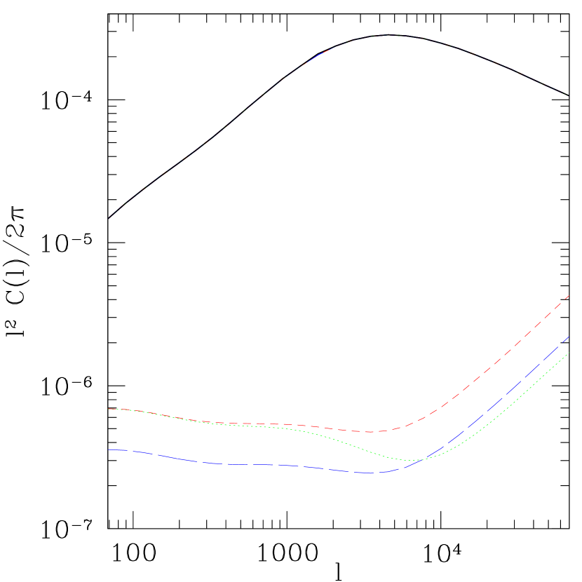
Figure 1: Statistical errors in the lensing power spectrum for three survey parameters. The upper black curve shows the shear power spectrum for source galaxies at $z=1$. The three lower curves show the statistical errors (the sum of sample variance and intrinsic ellipticity contribution) for three survey parameters described in the text. Since the PSF anisotropy can be of order 1%, its contribution ($\sim 10^{-4}$) would greatly exceed the statistical errors. It must be corrected by several orders of magnitude to fall below the statistical errors for these survey parameters.

To analyze the effect of errors on lensing statistics, we will consider the two-point correlation functions of the shear $\xi_{\gamma+}(\theta),\xi_{\gamma-}(\theta)$ and the shear power spectrum $C_{\gamma}(\ell)$. Other statistics often used in lensing measurements, such as the aperture mass variance and the top-hat shear variance, can be obtained by integrating the two-point correlation functions (Schneider et al., 2002), so there is no need to consider them in addition.

The contribution to the shear correlations per log interval in $\ell$ is $\ell^{2}C_{\gamma}(\ell)/2\pi$, which makes it an intuitive way to plot the shear power spectrum. Figure 1 shows this power spectrum for the (nonlinearly evolved) concordance $\Lambda-$CDM model, and the statistical errors on it for three choices of survey parameters. The statistical errors include sample variance, which dominates on large scales ($\ell$ below a few thousand) and the shot noise contribution of the intrinsic ellipticites of galaxies. The systematic errors should be smaller than the sum of these so as not to dominate the error budget.

The upper black curve shows the shear power spectrum for source galaxies at redshift $z=1$. The lowest statistical errors (long-dashed blue curve) are for a survey similar to that planned for the LSST, which covers half the sky: $f_{\rm sky}=0.5$, $n_{g}=40$ with rms intrinsic contribution to the shear $\sigma_{\gamma}=0.25$. The dashed red curve is for a ground based survey with smaller sky coverage: $f_{\rm sky}=0.1$, $n_{g}=40$. The dotted green curve shows the statistical error for a space based survey with $f_{\rm sky}=0.1$, $n_{g}=100$. The higher number density reduces the error at high $\ell$ compared to the ground based survey with the same sky coverage. For $\ell>10^{4}$, on sub-arcminute scales, the statistical error rises due to the intrinsic ellipticity contribution which has a white noise power spectrum (assuming the intrinsic ellipticities are uncorrelated and randomly oriented). However the statistical errors are roughly constant over the range of scales that provide the cosmological information ($100<\ell<10^{4}$). This is useful for setting the permissible level of residual systematics.

One of the main sources of error in the shear estimates comes from the convolution of the image by the point spread function (PSF). This function is known (albeit noisily) at the positions of the stars in the image. As the PSF varies across the image, one must interpolate this function to the positions of the galaxies. An incorrect model of the PSF leads to an error in the estimated (pre-seeing) galaxy shape and hence in the shear correlation. Coherent PSF patterns have non-zero two-point functions, which add to the lensing induced correlations in galaxy ellipticities. This systematic error can exceed statistical errors in lensing measurements if the PSF is not modeled sufficiently accurately (Hoekstra, 2004). We will not consider here errors due to removal of the PSF from the galaxy shapes if the PSF at the location of the galaxy is known correctly (e.g. Kaiser, Squires, & Broadhurst, 1995; Kaiser, 2000; Bernstein & Jarvis, 2002; Refregier & Bacon, 2003). We are only concerned here with the estimation of the PSF at each galaxy’s location.

PSF interpolation error has been one of the primary sources of systematic error in most of the lensing measurements published to date (errors in the shear calibration and redshift distribution are the other main sources). Given a model for PSF anisotropy we can calculate how well the power spectrum would need to be corrected to be well below the statistical errors. The statistical error curves in Figure 1 give a good indication of the upper limit on coherent residual systematic errors if they are not to dominate the error budget. Thus at $l\sim 1000$, or 10 arcminute scales, the coherent residual should be well below $0.001$ (so that its square is smaller than the statistical error curves). Generic models of PSF patterns do not exist; the amplitudes measured in current data (before any corrections) are in the range 1-10% with varying coherence scales. Telescopes that will be built with lensing as a primary science goal are expected to do better than these, and may have PSF modeling software like TinyTim for HST, but even for the best-designed telescope, the galaxy shapes will require correction using data on stars.

In this paper we describe two methods which in combination can remove the systematic effects of asymmetric PSFs in large imaging surveys. A method based on a principal component analysis (PCA) of the PSF was the subject of a recent paper (Jarvis & Jain, 2004). Essentially, it detects and models components of the PSF pattern which appear in many different images. For example, guiding errors have the same effect on every star in an exposure, so its pattern is a constant in $(x,y)$, with a coefficient which varies from exposure to exposure. The principal component corresponding to this is therefore a constant. Focus errors are similarly recurring; astigmatism produces a characteristic pattern when the telescope is slightly above focus, and the opposite pattern when below. That is, there is a fixed $(x,y)$ pattern which is modulated by a coefficient for each exposure. (There may be more than one principal component corresponding to focus if the variation is not quite linear as the telescope gets more out of focus.) In general, the principal components should model any pattern due to a recurrent physical cause. The second method discussed in this paper tackles PSF patters that no not recur in different exposures.

In §2, we outline the pipeline for lensing measurements to show where different sources of error enter. We quantify the residual systematic errors due to the PSF pattern after performing the PCA interpolation and show how they scale with survey area. We find that some components of the error scale as ${\rm Area}^{-1}$. However, other components of the error remain roughly constant even with this interpolation scheme. We discuss how these components are ones that do not recur across different exposures.

In §3, we show how to completely eliminate these non-recurring systematic errors by correlating only galaxy shapes measured on distinct exposures. Since the two- and three-point correlation functions encompass most of the lensing information that will be desired from current and future surveys, the combination of these two techniques will lead to the near elimination of systematic errors stemming from PSF interpolation.

In §4 we discuss the key requirements for a survey to keep residual systematics sufficiently small. We list the ingredients that determine these residuals and describe how to estimate them for planned surveys as well as from actual survey data. Future work needed to test and refine this approach is discussed.

2 Systematic Errors Due to PSF Interpolation

2.1 The Lensing Pipeline

We begin by outlining the pipeline used to estimate lensing statistics from images of the sky. This will help us identify the steps at which different errors enter and how new techniques can reduce certain errors. We will introduce the PCA technique below in step 3 on PSF interpolation and use it in subsequent sections to quantify residuals.

The lensing pipeline can be summarized in 5 main steps:

1. Detection of Stars and Galaxies

   Weak lensing surveys generally observe the same portion of the sky on several separate exposures. Each of these exposures are usually made up of multiple images, from the multiple CCD chips in the camera. These factors can make object detection and measurement somewhat complicated. Generally, one wants to stack all of the images for a given part of the sky to get the best signal-to-noise for detecting objects. However, if the shapes are measured from the stacked image, there are issues due to correlated noise from the image-combining algorithm, and even slight registration errors can lead to very significant errors in the shape measurements. Also, the PSF on the stacked image will be near the middle of the range of seeing values, so the signal-to-noise for the smallest galaxies may actually be worse on the stacked image than on the best-seeing images. Worse, the PSF pattern on the stacked image will change abruptly at the edge of every input exposure, so if there are large offsets in the original pointings, the PSF pattern will be impossible to model precisely.

   Therefore, we generally recommend detecting objects on a stacked image, but measuring the PSF and galaxy shapes on the images from the individual exposures. This will allow for good PSF interpolation, and the keep the pixel noise uncorrelated. If the image registration is good enough, one can centroid on the stacked image and use it for the individual measurements, which may improve the signal-to-noise of the shape estimates.

   In §3 we point out that using shapes from different exposures eliminates systematic errors due to certain PSF patterns; this also argues against stacking images to measure shapes. It will impact the optimal number of images to observe per location, which we discuss §3.1.

   For surveys with very many (more than about 10 or 20) exposures at each location, it may make sense to stack together several exposures which have roughly the same seeing and which are not (very) offset from each other. Each location would then have a smaller number of images for measuring shapes. For the purposes of this paper, the term exposure would then refer to these stacked images, rather than the original exposures.

   Finally, we remind the reader that the PSF can act as a matched filter for galaxies that are aligned in the same direction as it. This selection bias can introduce a systematic error. The error is eliminated by detecting galaxies which are as faint as possible, and then selecting according to an shape-independent signal-to-noise estimate. A similar error, which is more difficult to remove, is that galaxies are more likely to be blended along the direction of the PSF, which will bias galaxy shapes in the same direction.

2. Measurements of the PSF

   After identifying stars and galaxies in an image, the stars are used to measure various aspects of the PSF. Different analysis methods use different components of the PSF, but all methods measure the ellipticity and size at least. More sophisticated analyses require some higher order shape information as well. Since the PSF generally varies between different exposures as well as across the field, these values are measured as a function of the positions $\vec{\phi}^{(i)}$ of stars in exposure $i$.

   There are three systematic errors which may be introduced at this stage. First, small galaxies may be falsely identified as stars, which will lead to errors in the PSF estimates. Second, if the PSF is color dependent, the PSF measured by the stars may not be (exactly) the same as the PSF which has acted on the galaxies. This color error may be redshift dependent which would complicate tomography analyses. Similarly, if the detector response is slightly non-linear, the PSF of the bright stars may be different from the PSF of the faint galaxies.

3. Interpolation of the PSF

   We need to know the PSF at the location of the galaxies, which are the tracers of the lensing shear. Since the PSF is not measured at these locations, we need to interpolate the measurements from the locations of the stars. Here, we briefly describe how to do this using the principal component analysis (PCA) method (described in greater detail in Jarvis & Jain, 2004):

   For each exposure, $i$, we find a polynomial fit to the PSF measurements, $Q_{i}^{(m)}(\vec{\phi}^{(i)})$, where the order $m$ is given by the number of stars available for fitting: $(m+1)(m+2)/2\leq N_{*}$, and $\vec{\phi}^{(i)}$ is the position measured in the coordinate system of exposure $i$. In practice, one may want to use a separate polynomial for each chip to avoid smoothing over discontinuities at the chip boundaries.

   Next we take the patterns for all of the exposures and pointings, as quantified by the coefficients in the polynomials $Q_{i}$, and find the principal components of the variation. This will find the patterns that repeat over a significant number of the exposures. We sort the principal components according to how much they contribute to the total variation of the PSF patterns (i.e. the singular values). At some point the components will not be important for describing the patterns, so we choose some cutoff and only use the first $N_{\rm PC}$ components. (We will discuss how to determine this number below.) Thus, the PSF pattern for each exposure is described as a weighted sum of the various principal components:

   $$e_{\rm PSF}(\vec{\phi}^{(i)})=\sum_{k=1}^{N_{\rm PC}}a_{ik}P_{k}(\vec{\phi}^{(i)})$$ (1)

   where $i$ is the index number of the exposure, $e$ can represent the PSF ellipticity, or any other feature of the PSF, such as size or any higher order shape information, and $P_{k}$ is the $k$th principal component for the same quantity.

   We can then refine these principal components, $P_{k}$, using a higher order polynomial, by keeping the $a_{ik}$ coefficients fixed and using the stars in all of the exposures for the fit. For very large surveys, this allows us to use significantly higher order polynomials which more accurately describe the components.

4. Measurements of the galaxy shapes

   Given the relevant description of the PSF at the location of a galaxy, one can make an estimate of the galaxy’s shape before convolution by the PSF. Our methods for doing this are described in Bernstein & Jarvis (2002), but there are other methods for this step as well. For the purposes of this paper, we will assume that the only errors introduced here are the measurement noise and the intrinsic shape noise of the galaxy. That is, if the knowledge of the PSF were perfect, we assume that this step would then produce perfectly unbiased estimates of the shear at each galaxy’s location.

   In reality, there may be systematic errors due to the dilution correction (the effect of the size of the PSF on galaxy shapes; c.f. Hirata & Seljak, 2003) or the shear calibration (the response of the distribution of galaxy ellipticities to the shear). These errors lead to multiplicative errors in the shear two-point correlations. We discuss in §4 how the improved PSF interpolation we describe would reduce the dilution errors as well. Recent studies (Huterer et al., 2005; Guzik & Bernstein, 2005) show that the impact of these errors on cosmological parameter estimation is less severe than the additive errors due to PSF anisotropy, as they can be self-calibrated from the data..

5. Correlation of the shear estimates and comparison to theory

   The lensing shear information is contained primarily in the two- and three-point shear correlation functions. In fact, most other shear statistics, such as the shear variance and the aperture mass variance and skewness, can be expressed as integrals over these functions. Exceptions include the convergence probability distribution function (Zhang & Pen, 2005), peak statistics (Jain & van Waerbeke, 2000; Miyazaki et al., 2002) and topology measures (Matsubara & Jain, 2001; Sato et al., 2001, 2003), which contain more information about the shear than is contained in its low-order correlations.

   There are two two-point shear correlation functions:

   $$\xi_{+}(\theta) =\left\langle\gamma(\vec{\phi})\gamma^{*}(\vec{\phi}+\vec{\theta})\right\rangle$$ (2)

   $$\xi_{-}(\theta) =\left\langle\gamma(\vec{\phi})\gamma(\vec{\phi}+\vec{\theta})\right\rangle$$ (3)

   where ^∗ indicates complex conjugate of the complex-valued shear estimate, and the shears are measured relative to the line joining the two galaxies. Likewise, there are four three-point shear correlation functions which are a function of the size and shape of the triangle connecting the three galaxies.

   Since other statistics may be derived from these, we take the correlation functions to be the final product of the lensing pipeline which is then used to constrain cosmology. For tomography applications, the correlation functions are measured as functions of redshift bins as well as the angular separation. The following discussion of the errors would then refer to the errors in the correlation functions for each pair (or triplet) of redshift bins.

   The estimation of cosmological parameters from the measured shear correlations relies on the use of redshift information. Errors in the estimated redshift bins (or the overall distribution of redshifts for non-tomographic applications) are an important systematic error which may be introduced at this point. Accurately calibrating the redshifts is a big concern for upcoming large cosmic shear surveys (Ma, Hu & Huterer, 2005; Huterer et al., 2005). Spectroscopic sub-samples that extend to high redshifts may be necessary to calibrate the redshift distribution, though Mandelbaum et al. (2005) show how to some extent it can be calibrated from the data.

   There may also be systematic errors introduced by the theoretical predictions. In particular, current estimates of the non-linear power spectrum may have errors of order 5% at scales of several arcminutes (Smith et al., 2003), or even larger for quintessence models (Klypin, 2003). (See Linder & White, 2005 for an improved prescription for generic dark energy cosmologies.) On small scales it is also necessary to consider baryonic physics (White, 2004; Zhan & Knox, 2004) and higher order effects, e.g. to account for the fact that galaxy shape measurements estimate the reduced shear $g=\gamma/(1-\kappa)$, not the shear $\gamma$ directly (White, 2005; Dodelson et al., 2005). Theoretical predictions which do not correctly take this into account would introduce an error on small scales.

We have seen that there are systematic errors which may be introduced in every step of the lensing pipeline. The errors from the PSF interpolation step have often been considered the most difficult to remove due to the limited number of stars per exposure. The most problematic of the other errors are the shear calibration and the redshift calibration. There is ongoing work aimed at limiting the impact of these errors on cosmological parameter estimation from future lensing data. However, they are not the focus of this paper; henceforth we restrict our discussion to the PSF interpolation errors.

2.2 Residual Systematic Errors after PCA Interpolation

We now want to determine what the residual systematic errors in the estimates of the correlation functions are, due to imperfect PSF interpolation. Let the estimated shear in exposure $i$ at position $\vec{\phi}^{(i)}$ be

$$\hat{\gamma}(\vec{\phi}^{(i)})=\gamma_{\rm grav}(\vec{\phi}^{(i)})+\epsilon_{\rm intrinsic}(\vec{\phi}^{(i)})+\epsilon_{\rm meas}(\vec{\phi}^{(i)})+\epsilon_{\rm PSF}(\vec{\phi}^{(i)})$$ (4)

where $\gamma_{\rm grav}$ is the lensing signal, $\epsilon_{\rm intrinsic}$ is the noise due to the intrinsic shape of the galaxies, $\epsilon_{\rm meas}$ is the statistical error in the measurement from the photon shot noise, and $\epsilon_{\rm PSF}$ is the error in the shear estimate due to uncorrected PSF contamination.

The systematic errors from the PSF interpolation enter through the term $\epsilon_{\rm PSF}$, which arises from errors in the PSF ellipticity. Using equation 1, which expands it in principal components, we can write $\epsilon_{\rm PSF}$ as:

$$\epsilon_{\rm PSF}(\vec{\phi}^{(i)})=\frac{1}{\cal R}\sum_{k\leq N_{\rm PC}}\left[\delta a_{ik}P_{k}(\vec{\phi}^{(i)})+a_{ik}\delta P_{k}(\vec{\phi}^{(i)})\right]+\frac{1}{\cal R}\sum_{k>N_{\rm PC}}a_{ik}P_{k}(\vec{\phi}^{(i)})$$ (5)

where $\delta$ refers to the error in the estimate of a quantity, and the last sum includes all of the patterns which are not modeled by the PCA, including any completely random effects which do not recur in multiple exposures. ${\cal R}$ represents the conversion from ellipticity to shear, which Bernstein & Jarvis (2002) refer to as responsivity. When using this technique for other properties of the PSF besides ellipticity (size for example), ${\cal R}$ would be the corresponding mean effect that errors in the measurement have on the net shear estimates from the galaxy shapes.

We will refer to the estimates of the two-point correlation function from observations of galaxies on two exposures, $i$ and $j$ as:

$$\hat{\xi}^{(i,j)}(\theta)=\left\langle\hat{\gamma}(\vec{\phi}^{(i)})\hat{\gamma}(\vec{\phi}^{(j)}+\vec{\theta})\right\rangle$$ (6)

where we omit the $+$ and $-$ subscripts, both here and in much of the further discussion, leaving the appropriate conjugation or not in the two cases implied.

The statistical errors from the measurement noise and intrinsic ellipticities are well understood. We now look at what can contribute to the systematic PSF contamination, $\epsilon_{\rm PSF}$, and how that propagates to $\hat{\xi}^{(i,j)}$. The errors in the three-point function are completely analogous, so it is sufficient to only refer to the two-point function here.

1. Errors in the principal components, $P_{k}$

   There will be errors in the estimates of the $P_{k}$ functions due to the simple fact that we constrain them with a finite number of stars. These lead to systematic errors in the correlation functions, since we use the same principal components for all of the exposures, so the errors in the $P_{k}$ repeat for every pair of galaxies that is used to calculate the correlation function.

   If the error in each estimated $P_{k}$ is $\delta P_{k}$, then the propagated error in the correlation function due to this is (from Equations 5 and 6):

   $$\delta\hat{\xi}_{(\ref{error_p})}^{(i,j)}=\frac{1}{{\cal R}^{2}}\sum_{k,\ell\leq N_{\rm PC}}a_{ik}a_{j\ell}\left\langle\delta P_{k}(\vec{\phi}^{(i)})\delta P_{\ell}(\vec{\phi}^{(j)}+\vec{\theta})\right\rangle$$ (7)

2. Unmeasured principal components

   The above analysis only included a finite number of principal components, $N_{\rm PC}$. Any PSF variation that is described by components of lower significance than these has been completely unmodeled. Therefore, all of this PSF power will still be uncorrected in the galaxy shapes, which will lead to a systematic error in the shear estimates:

   $$\delta\hat{\xi}_{(\ref{error_unmeasured})}^{(i,j)} =\frac{1}{{\cal R}^{2}}\sum_{k>N_{\rm PC}}\Bigg{(}2\ \sum_{\ell\leq N_{\rm PC}}a_{ik}a_{j\ell}\left\langle P_{k}(\vec{\phi}^{(i)})\delta P_{\ell}(\vec{\phi}^{(j)}+\vec{\theta})\right\rangle$$

   $$\qquad\qquad\quad\quad+\sum_{\ell>N_{\rm PC}}a_{ik}a_{j\ell}\left\langle P_{k}(\vec{\phi}^{(i)})P_{\ell}(\vec{\phi}^{(j)}+\vec{\theta})\right\rangle\Bigg{)}$$ (8)

   $$\approx\frac{1}{{\cal R}^{2}}\sum_{k>N_{\rm PC}}a_{ik}a_{jk}\left\langle P_{k}(\vec{\phi}^{(i)})P_{k}(\vec{\phi}^{(j)}+\vec{\theta})\right\rangle$$ (9)

   where $a_{ik}$ refers to the values that the coefficients for the unmeasured components would have if they were included in the analysis. The dominant terms in this expression will typically be the autocorrelation terms as written in Equation 9; however, it is possible that there could be significant correlations with either other unmeasured components or the errors in the measured components as shown in Equation 8.

3. Non-recurring contributions to the PSF pattern

   Some portion of the PSF pattern is completely random and uncorrelated between different exposures, e.g. atmospheric effects. These non-recurring contributions will remain as a systematic error in the shear correlations since they can have spatial structure. Wittman (2005) has recently measured the atmospheric contribution to PSF errors from the Subaru telescope, while Kaiser, Tonry, & Luppino (2000) modeled its spatial and temporal coherence. The actual level of atmospheric contribution will depend on details of the instrument and observing strategy. Here we will consider the atmosphere as well as non-recurring contributions from the instrument in one category of PSF errors.

   These could be viewed as a subset of the unmeasured principal components described above, since the information here must be contained in a complete principal component analysis with $N_{\rm PC}$ equal to the total number of exposures. These uncorrelated contributions would be described by the myriad very low significance components which constitute most of those neglected by using a (much) lower $N_{\rm PC}$. However, we choose to make them a separate item to point out that these contributions are completely uncorrelated from one exposure to another, which make them a qualitatively different type of error. In particular, this means that $\langle a_{ik}a_{jk}\rangle=0$ for $i\neq j$, so the systematic error only occurs for estimates of $\xi$ with $i=j$:

   $$\delta\hat{\xi}_{(\ref{error_atm})}^{(i,i)}=\frac{1}{{\cal R}^{2}}a_{{\rm atm},i}^{2}\left\langle P_{\rm atm}^{(i)}(\vec{\phi}^{(i)})P_{\rm atm}^{(i)}(\vec{\phi}^{(i)}+\vec{\theta})\right\rangle$$ (10)

   where $P_{\rm atm}^{(i)}$ is the portion of the PSF pattern which is uncorrelated with that from any other exposure.

4. Errors in the coefficients $a_{ik}$

   There will be errors in the estimates of the $a_{ik}$ coefficients as well, since they will be constrained by the finite number of stars in each exposure. These errors lead to systematic errors in the correlation function, since the amount of correction on the galaxies for each principal component will be slightly wrong. This will then add a little bit of the correlation functions of the components to the shear correlation function:

   $$\delta\hat{\xi}_{(\ref{error_a})}^{(i,i)}=\frac{1}{{\cal R}^{2}}\sum_{k,\ell\leq N_{\rm PC}}{\rm Cov}\left(a_{ik},a_{i\ell}\right)\left\langle P_{k}(\vec{\phi}^{(i)})P_{\ell}(\vec{\phi}^{(i)}+\vec{\theta})\right\rangle$$ (11)

   Note that, like the previous systematic, this systematic is nonzero only for estimates of $\xi$ with $i=j$, since the errors on the coefficients are uncorrelated between exposures.

2.3 Scaling of Systematics with Survey Parameters

Surveys with degree sized fields of view (FOV), covering total area of 1000 square degrees or larger, are likely to have enough exposures and stars to make accurate corrections to PSF anisotropy. Here we quantify the residual PSF systematics described above and discuss their possible impact on survey strategy.

The following parameters constitute our description of a lensing survey.

• Field of view, in steradians: $\Omega_{\rm FOV}$

• Number of pointings: $N_{\rm point}$

• Number of exposures per pointing: $N_{\rm exp}$

• Mean number of stars per exposure: $\langle N_{*}\rangle\equiv N_{*}=n_{*}\ \Omega_{\rm FOV}$

• Number of significant principal components: $N_{\rm PC}$

The survey size is given by the number of pointings as: $\Omega_{\rm S}=N_{\rm point}\Omega_{\rm FOV}$. For PSF measurement $N_{*}$ includes only those stars that have well measured shapes, and which are robustly identified as stars. Interloping small galaxies are an additional concern if one tries to push the stellar locus too close to the galaxy locus of the size-magnitude diagram. The number of significant principal components used to describe the recurring PSF pattern, $N_{\rm PC}$, will not likely be known in advance of the data. In fact, it is still variable after obtaining data; we describe how to determine a good value for it in §2.3.1.

We will make the simplifying and conservative assumption that all exposures in a given part of the sky are centered on the same point, so they do not sample the PSF on different parts of the camera. Hence the total number of PSF measurements is $N_{*}N_{\rm point}$. These are used to measure the $N_{\rm PC}$ principal components. The maximum order of the polynomial that can be used for each principal component is then of roughly $(N_{*}N_{\rm point}/N_{\rm PC})^{1/2}$, which can be much larger than the order possible by using just the stars in a single exposure.

2.3.1 Scaling of Errors 1 and 2

The magnitude of the errors in the principal components scales according to the total number of stars used to constrain each component. Since all of the stars in the survey need to jointly constrain $N_{\rm PC}$ components, we have

$$|\delta P_{k}(\vec{\phi})|\propto\left(\frac{N_{\rm PC}}{N_{*}N_{\rm point}}\right)^{1/2}$$ (12)

The systematic error $\delta\hat{\xi}_{(\ref{error_p})}^{(i,j)}$ will then scale as

$$\delta\hat{\xi}_{(\ref{error_p})}^{(i,j)}\propto N_{\rm PC}\ |\delta P(\vec{\phi})|^{2}\propto\frac{N_{\rm PC}^{2}}{N_{*}N_{\rm point}}$$ (13)

since each element in the sum for $\delta\hat{\xi}_{(\ref{error_p})}^{(i,j)}$ in Equation 7 is quadratic in the $\delta P_{k}$ functions (assuming that the cross-terms involving different principal components are negligible). As survey size increases (increasing $N_{\rm point}$), this systematic error will decrease even faster than the statistical errors in the shear, which decrease as $N_{\rm point}^{-1/2}$, presuming that the PC patterns do not evolve as the survey progresses.

The error due to the neglected principal components, $\delta\hat{\xi}_{(\ref{error_unmeasured})}^{(i,j)}$, will only decrease if we increase $N_{\rm PC}$, since the largest neglected components will then have smaller rms amplitude. However, increasing $N_{\rm PC}$ will increase the previous error, since each principal component will be less well measured. In an ideal analysis, the number of principal components would be set so that the systematic errors for each of these two factors is stationary in the number of components. That is, the improvement due to adding an additional component should exactly offset the loss due to the other components being slightly less well measured. In general, it is not easy to determine at what $N_{\rm PC}$ this will happen. One needs to look at some measure of the contamination as a function of $N_{\rm PC}$ to find the minimum total contamination. We discuss a few such measures in §4.

If such a procedure is done, then the amplitude of the first neglected component will scale approximately as

$$|P_{N_{\rm PC}+1}(\vec{\phi})|\propto\left(\frac{N_{\rm PC}}{N_{*}N_{\rm point}}\right)^{1/2}.$$ (14)

Furthermore, in our CTIO survey data, we have found that the large-$k$ asymptotic behavior of $|P_{k}|$ is

$$|P_{k}(\vec{\phi})|\propto e^{-\alpha k}$$ (15)

with $\alpha$ of order $0.02$. Therefore, we can estimate $\delta\hat{\xi}_{(\ref{error_unmeasured})}^{(i,j)}$ as

$$\delta\hat{\xi}_{(\ref{error_unmeasured})}^{(i,j)} \propto\sum_{k>N_{\rm PC}}|P_{k}(\vec{\phi})|^{2}\approx\frac{1}{2\alpha}|P_{N_{\rm PC}+1}(\vec{\phi})|^{2}$$ (16)

$$\propto\frac{N_{\rm PC}}{\alpha N_{*}N_{\rm point}}$$ (17)

Assuming the asymptotic behavior is relatively generic and that the necessary increase in $N_{\rm PC}$ occurs significantly more slowly than the increase in $N_{\rm point}$, both systematics would scale as $N_{\rm point}^{-1}$.

However, we should point out that one is also limited by the constraint that $N_{\rm PC}<N_{*}$, otherwise the coefficients $a_{ik}$ cannot be measured: so if too many principal components become important, it will eventually become impossible to include all of them, and $\delta\hat{\xi}_{(\ref{error_unmeasured})}^{(i,j)}$ will not scale as $N_{\rm point}^{-1}$ any further. Thus, it is important in designing a survey to try to minimize the number of sources of PSF variation to keep the number of principal components reasonably low.

2.3.2 Scaling of Errors 3 and 4

The error from the atmosphere’s PSF, $\delta\hat{\xi}_{(\ref{error_atm})}^{(i,i)}$, is essentially constant with survey size. Some of the atmosphere’s PSF pattern will be modeled by the various principal components, but most of the PSF power will remain as a systematic error, especially the high order power, which will almost always be completely different from the high order power of the PC’s. In particular, the atmosphere’s pattern on scales smaller than the stellar separation cannot be modeled by the PCA or any other method. The magnitude of this contribution seems to be relatively small for current surveys. But for upcoming larger surveys, its contribution may become dominant over the residuals from the coherent patterns due to the telescope. Space-based surveys will not have this contribution, although it is possible that they will have other sources of PSF patterns which are uncorrelated between exposures.

The errors in the coefficients $a_{i,k}$ do not scale with the number of pointings, since they are constrained only by the stars in a single exposure. For each exposure, $i$, there are $N_{*}$ stars which are used to constrain $N_{\rm PC}$ coefficients. Take the stars in an exposure to be numbered $m=1..N_{*}$ with positions $\vec{\phi}_{m}$, shapes $e_{m}$, and shape uncertainties $\sigma_{m}$. Also, define $A$ to be the vector of coefficients for that exposure ($A_{k}=a_{i,k}$), define a vector $E$ with $E_{m}=e_{m}/\sigma_{m}$, and define a matrix $Q$ with $Q_{m,k}=P_{k}(\vec{\phi}_{m})/\sigma_{k}$. Then the least-squares solution for $A$ is:

$$A =(Q^{T}Q)^{-1}(Q^{T}E)$$ (18)

$${\rm Cov}(A) =(Q^{T}Q)^{-1}$$ (19)

If $N_{*}<N_{\rm PC}$, then $Q^{T}Q$ is singular and the errors on A are infinite. If $N_{*}=N_{\rm PC}$ then there is some combination of coefficients whose error is proportional to the largest $\sigma_{m}$. If we sort the stars by $\sigma_{m}$, so that the largest $\sigma_{m}$ is at $m=N_{*}$, then

$$\sigma(\tilde{a})=K\sigma_{N_{*}}$$ (20)

where $\tilde{a}$ is the least well measured linear combination of coefficients and $K$ is a constant which depends on the values of $P_{k}(\vec{\phi}_{m})$. $K$ is generally of order the rms value of $P_{k}(\vec{\phi}_{m})$, but it can be arbitrarily larger for unfortunate sampling of the principal components. Finally, if $N_{*}>N_{\rm PC}$ (the usual case), then it can be shown that

$$\sigma(\tilde{a})\geq K^{\prime}\left(\sum_{k\geq N_{\rm PC}}\frac{1}{\sigma_{k}^{2}}\right)^{-1/2}$$ (21)

where the sum is over the $(N_{*}-N_{\rm PC}+1)$ least well-measured stars. Since $\sigma_{k}\propto 1/\nu$, where $\nu$ is the signal-to-noise of the star, the sum in the above formula is dominated by the highest signal-to-noise stars. Thus the overall error scales roughly as the shape error of the $N_{\rm PC}$-th brightest star. The fainter stars do not help very much. Since $\delta\hat{\xi}_{(\ref{error_a})}^{(i,i)}$ contains a sum over the elements of ${\rm Cov}(A)$, it scales similarly.

3 Multi-exposure Correlation Functions

In the preceding section, we found two contributions to the systematic error in the correlation functions which do not scale with the survey size. However, notice that both of these, $\delta\hat{\xi}_{(\ref{error_atm})}^{(i,i)}$ and $\delta\hat{\xi}_{(\ref{error_a})}^{(i,i)}$ only exist for estimates of the correlation function which use shear estimates from the same exposure ($i=j$).

There is a simple way to eliminate such systematic errors in the correlation function: for each pair of galaxies used in estimating the two-point function, use galaxy shapes measured from different exposures. In other words, only use pairs with $i\neq j$. Since the atmospheric component of $\epsilon_{\rm PSF}$ and that from the errors in the coefficients are uncorrelated between exposures $i$ and $j$, there is no systematic bias in the estimates of the correlation function. We have thus used the fact that the atmosphere has spatial coherence in any given exposure, but gets uncorrelated rapidly between distinct exposures (as long as they are not taken in immediate succession). The same holds for some types of instrumental systematics which are not correlated between exposures taken on different nights. The systematic errors eliminated by this technique are what we have been calling $\delta\hat{\xi}_{(\ref{error_atm})}^{(i,i)}$ and $\delta\hat{\xi}_{(\ref{error_a})}^{(i,i)}$. So for these two components of the error, $\delta\hat{\xi}=0$.

For the three-point (or $n-$point) correlation function, the same argument holds as long we have at least three (or $n$) exposures. With the shapes all taken from different exposures, the systematic errors from the atmosphere and the coefficient estimates are eliminated, leaving only the errors from the PC measurements and the neglected PCs to contribute to the systematic error.

By $\delta\hat{\xi}$, we have been referring to a systematic error, or bias; that is, a change in the expectation value relative to the correct value. So correlating across multiple exposures results in no systematic error from the effects we have numbered 3 and 4. However, these errors (all four, actually) also contribute to the statistical error in $\xi$, since the variance of $\xi$ due to these two errors does not vanish. This contribution to the statistical error has yet to be accurately estimated, but we expect it to be small compared to the sample variance plus intrinsic ellipticity errors ($\epsilon_{\rm intrinsic}$ from Equation 4).

Wittman (2005) used a set of exposures of a single field imaged with the Subaru telescope to estimate the atmospheric contribution. This is a concern on arcminute scales or smaller, for which the PSF correction may not be accurate even with PCA interpolation if the PSF pattern is non-recurrent. Wittman (2005) finds a contribution to the shear correlation of order $10^{-5}$ on arcminute scales. This may be compared to the contribution from intrinsic ellipticities, which is of order $10^{-3}$, but scales inversely with the total number of galaxy pairs. The atmospheric contribution scales inversely with the number of independent coherent patches, which depends on the coherence scale of the atmosphere. Unless this scale is much larger than an arcminute, the atmospheric contribution will be comparatively small. The contribution of the other three errors to the statistical error budget is also likely to be small, but it needs to be estimated for planned surveys.

3.1 Optimal Number of Exposures per Pointing

How many exposures should one take per pointing? We have advocated multiple exposures in the discussion above to be able to use galaxies in different exposures to measure shear correlations. While this eliminates certain systematic errors, by omitting the $i=j$ terms in the correlation function estimates, we are losing some information.

Assume each pair of galaxies which are being used for the two-point correlation function are each observed on $N_{\rm exp}$ exposures and have a measurement error, $\epsilon_{\rm meas}$, on each exposure equal to $\sigma\sqrt{N_{\rm exp}}$ (so the measurement error on a stacked image would be $\sigma$). The variance of $\xi$ when the $i=j$ pairs are neglected is found to be:

$$Var(\xi)=\frac{1}{N_{\rm pair}}\left(\sigma_{\gamma}^{4}+2\sigma^{2}\sigma_{\gamma}^{2}+\frac{N_{\rm exp}\sigma^{4}}{(N_{\rm exp}-1)^{2}}\right)$$ (22)

For well measured galaxies, the last term is negligible (assuming $N_{\rm exp}\geq 2$); however, for faint galaxies, it becomes important. One generally limits one’s measurements to galaxies with $\sigma\lesssim\sigma_{\gamma}\approx 0.25$, since the measurments of fainter galaxies will often be unstable. For $\sigma\approx\sigma_{\gamma}$, we see that the fractional increase in the noise from omitting the $i=j$ pairs is $N_{\rm exp}/3(N_{\rm exp}-1)^{2}$, which is somewhat significant for only 2 exposures, but is small for 5 exposures.

If the shape uncertainties vary significantly between exposures, then our approximation that each shear error is $\sigma\sqrt{N_{\rm exp}}$ would be incorrect. A more careful analysis in this case suggests using enough exposures so that there are at least 2 or 3 with “good” measurements of the shapes. For typical variations in the seeing quality, 5 exposures is probably still sufficient.

On the other hand, with large $N_{\rm exp}$, the measurements of the shapes on each exposure becomes harder relative to the measurement on a stacked image. If the signal-to-noise on an individual image drops to near unity, the measurements may fail to provide any kind of useful value. Even signal-to-noise values of 5 or 10 often create problems. So to avoid having to discard many galaxies which would be measurable on a stacked image, we definitely want to limit $N_{\rm exp}$ to at most 10 or so.

Therefore, we suggest a minimum of 5 and a maximum of about 10 exposures per pointing for mesurements of shear correlations. For surveys planning to take very many exposures per pointing, one would want to stack subsets of the exposures into 5-10 stacked images and treat these sub-stacks as the exposures to which we have been referring. Sorting the original images by seeing radius before stacking would probably be the best strategy in order to not wash out the best-seeing images for at least 2 or 3 of the sub-stacks.

3.2 Effect on Recurring Principal Components

The multi-exposure technique may also help the first two systematic errors somewhat. The equations for these errors have terms with $\left\langle a_{ik}a_{j\ell}\right\rangle$ in them. With $i\neq j$, the two coefficients will often be uncorrelated, so this reduces to $\left\langle a_{ik}\right\rangle\left\langle a_{j\ell}\right\rangle$. Then, if the coefficients for either component $k$ or $\ell$ have zero expectation value, then these terms will vanish as well. Even if the expectation values are not exactly zero, they may often be much smaller than the rms, so the $i\neq j$ terms may still be much smaller than the autocorrelation $i=j$ terms.

Not all coefficients will be uncorrelated between different exposures. For example, for ground-based telescopes, some components may correspond to telescope flexure when the telescope points in a particular direction. If a given location is always observed at similar hour angle, the coefficients for these components will be correlated.

4 Discussion

This paper has been concerned with the effect of PSF anisotropy patterns on systematic errors in weak lensing surveys. We have suggested the use of galaxy shapes measured in distinct exposures to estimate shear correlations as a way of eliminating the systematic error due to non-recurrent PSF patterns. Jarvis & Jain (2004) showed that recurrent PSF patterns can be accurately measured using a Principal Component Approach. By using these two techniques in lensing pipelines, systematic errors due to generic PSF patterns can be interpolated (and therefore corrected) to high accuracy.

In planning a large-area cosmic shear survey, we have shown that the key factors that enable accurate PSF corrections are: sufficiently many well-measured stars in all parts of the sky; 5-10 exposures per pointing; sufficiently few important principal components, which cannot exceed the number of stars per exposure. In addition, the principal components can be estimated better if dense stellar fields are imaged on regular intervals, and if there are few changes in the instrument over the course of the survey (as these can introduce new principal components).

Another consideration for minimizing the number of important principal components is to keep the observing conditions as stable as possible. For each underlying physical cause of PSF variation, one can essentially do a Taylor expansion of the PSF pattern with respect to that variable. The PCA will need a separate component for each term in the Taylor expansion which has a significant amplitude. Thus, one should try to keep such variations (eg. focus error, component misalignments, mirror flexure, etc.) small enough that one or two terms in the expansion are sufficient to adequately describe the effect on the PSF pattern. One can estimate what limits are sufficient through spot-diagram ray-tracing programs.

The second goal of this paper was to provide a formalism to estimate residual systematics due to PSF errors. The ingredients needed to apply our formalism are an estimate of typical PSF power spectra and of the number of significant principal components of PSF patterns. For planned surveys, this is best accomplished by generating PSF patterns in a given exposure by ray tracing through the telescope optics. Mock surveys can then be generated by modeling the atmosphere and the variation of instrumental parameters over the course of the survey. The resulting models of PSF patterns can be used with the formalism of §2 to find telescope parameters and survey strategy that minimize residual systematics. The difficulty in getting reliable estimates of residual systematics will be in including all relevant factors which may affect the PSF, many of which may be subtle and hard to anticipate. But the benefit of such an exercise is the ability to optimize instrument and survey parameters for lensing measurements.

Further, once data is taken, comparison of the measured principal components with the models will help validate the error analysis. Our formalism can be applied to survey data to estimate residual systematic errors. If systematics turn out to be significant, empirical estimation allows one to incorporate them in the error budget for cosmological parameters. In addition, the following tests provide independent checks of the estimate of systematic errors from survey data (note that at least the latter two tests can be applied to model PSF patterns for planned surveys as well):

• Stellar ellipticity correlations

  For analysis methods where the corrected stars are not degenerately round, the two- and three-point correlation functions of the corrected stars can be a measure of how well the interpolation is removing the systematic contributions to the correlation. For a better check, one can perform the PSF corrections with only half the stars, and look at the resulting correlations of the other half.

• Cross-correlation of galaxies with foreground stars

  This will provide a somewhat more direct measure of the contamination from the interpolation, since the galaxies use the interpolated PSF. Again, one can split the stars in half for a better check.

• E/B mode analysis

  The shear field can be decomposed into curl-free (E) and divergence-free (B) modes (Schneider et al., 1998; Crittenden et al., 2001). Most PSF effects have roughly equal power in the E and B-modes, while the lensing signal is (almost) only in the E-mode. So any residual PSF contamination should show up in the B-mode. However, there are some cosmological sources of B-mode power (Crittenden et al., 2001; Schneider et al., 2002), so when these become important, this check will only provide an upper limit to the contamination due to the PSF and other systematic effects (e.g. Vale et al 2004).

• Higher order correlations

  Higher order correlation functions, in particular the three-point function, provide some independent checks on systematic errors. The three-point function of the gravitational shear vanishes at lowest order in the density in the quasilinear regime, so it is non-zero only at fourth-order in the density, but it would likely have a third order contribution from systematic errors. That is, the relative contribution of systematics could be higher than it is in the two-point function. Further, there are multiple three-point functions that contain B-mode contributions, which would in general behave differently from the two-point functions. The three-point function also has a shape dependence that should reveal its gravitational origin and depends somewhat differently on cosmological parameters than the two-point function (Bernardeau et al. 1997; Takada & Jain 2004).

Finally we note that the methods described here would reduce systematic errors due to the correction for the size of the PSF in addition to those due to the anisotropic PSF described above. A round PSF smoothes the images of the galaxies, making them appear less elliptical. A multiplicative “dilution correction” (part of the shear polarizability in the KSB formalism) is therefore needed to obtain the pre-seeing shape of the galaxies. PCA interpolation provides better estimates of the size of the PSF, which is needed for this correction. And the muti-exposure trick would eliminate the contribution of dilution errors due to non-recurrent patterns in the shear correlation functions. A detailed study of the resulting improvements is left for further work.

References

- Bernstein & Jarvis (2002) Bernstein, G. & Jarvis, M. 2002, AJ, 123, 583
- Bernardeau et al. (1997) Bernardeau, F., van Waerbeke, L., & Mellier, Y. 1997, A&A, 322, 1
- Crittenden et al. (2001) Crittenden, R., Natarajan, P, Pen, U., & Theuns, T., 2001, ApJ, 559, 552
- Abbott et al. (2005) Abbott, T. et al. 2005, arXiv:astro-ph/0510346
- Dodelson et al. (2005) Dodelson, S., Shapiro, C., & White, M. 2005, arXiv:astro-ph/0508296
- Golub & van Loan (1996) Golub, G. & van Loan, C., 1996, Matrix Computations, Johns Hopkins University Press
- Guzik & Bernstein (2005) Guzik, J., & Bernstein, G. 2005, Phys. Rev. D, 72, 043503
- Hirata & Seljak (2003) Hirata, C. & Seljak, U. 2003, MNRAS, 343, 459
- Huterer et al. (2005) Huterer, D., Takada, M., Bernstein, G., & Jain, B. 2005, arXiv:astro-ph/0506030
- Hoekstra (2004) Hoekstra, H. 2004, MNRAS, 347, 1337
- Jain & van Waerbeke (2000) Jain, B. & van Waerbeke, L., 2000, ApJ, 530, 1
- Jarvis & Jain (2004) Jarvis, M. & Jain, B. 2004, astro-ph/0412234
- Kaiser (2000) Kaiser, N. 2000, ApJ, 537, 555
- Kaiser (2004) Kaiser, N. 2004, Proceedings of the SPIE, 5489, 11
- Kaiser, Squires, & Broadhurst (1995) Kaiser, N., Squires, G., & Broadhurst, T. 1995, ApJ, 449, 460
- Kaiser, Tonry, & Luppino (2000) Kaiser, N., Tonry, J., & Luppino, G. 2000, PASP, 112, 768
- Klypin (2003) Klypin, A., Macciò, A., Mainini, R., Bonometto, S., 2003, ApJ, 599, 31
- Lampton et al. (2002) Lampton, M., et al. 2002, Proceedings of the SPIE, 4849, 215
- Linder & White (2005) Linder, E. V., & White, M. 2005, arXiv:astro-ph/0508401
- Ma, Hu & Huterer (2005) Ma, Z., Hu, W., & Huterer, D. 2005, arXiv:astro-ph/0506614
- Mandelbaum et al. (2005) Mandelbaum, R. et al., 2005, MNRAS, 361, 1287
- Matsubara & Jain (2001) Matsubara, T., & Jain, B. 2001, ApJ, 552, L89
- Miyazaki et al. (2002) Miyazaki, S., et al. 2002, ApJ, 580, L97
- Refregier & Bacon (2003) Refregier, A. & Bacon, D. 2003, MNRAS, 338, 48
- Sato et al. (2001) Sato, J., Takada, M., Jing, Y. P., & Futamase, T. 2001, ApJ, 551, L5
- Sato et al. (2003) Sato, J., Umetsu, K., Futamase, T., & Yamada, T. 2003, ApJ, 582, L67
- Schneider et al. (1998) Schneider, P., van Waerbeke, L., Jain, B., & Kruse, G. 1998, MNRAS, 296, 873
- Schneider et al. (2002) Schneider, P., van Waerbeke, L., & Mellier, Y., 2002, A&A, 389, 729
- Smith et al. (2003) Smith, R., Peacock, J, Jenkins, A., White, S., Frenk, C., Pearce, F., Thomas, P., Efstathiou, G., & Couchman, H., 2002, MNRAS, 341, 1311
- Starr et al. (2002) Starr, B.; Claver, C.; Wolff, S.; Tyson, J. A.; Lesser, M.; Daggert, L.; Dominguez, R.; Gomez, R. R. Jr.; Muller, G. 2002, Proceedings of the SPIE, 4836, 228
- Takada & Jain (2004) Takada, M., & Jain, B. 2004, MNRAS, 348, 897
- Vale et al. (2004) Vale, C., Hoekstra, H., van Waerbeke, L., & White, M. 2004, ApJ, 613, L1
- White (2004) White, M. 2004, Astroparticle Physics 22, 211
- White (2005) White, M. 2005, Astroparticle Physics, 23, 349
- Wittman (2005) Wittman, D. 2005, arXiv:astro-ph/0509003
- Zhan & Knox (2004) Zhan, H. & Knox, L. 2004, ApJ, 616, L75
- Zhang & Pen (2005) Zhang, T. & Pen, U., 2005, arXiv:astroph/0503064