ESO Imaging Survey: Optical follow-up of 12 selected XMM-Newton fields^,

This paper presents the data recently released for the XMM-Newton/WFI survey carried out as part of the ESO Imaging Survey (EIS) project. The aim of this survey is to provide optical imaging follow-up data in $BVRI$ for identification of serendipitously detected X-ray sources in selected XMM-Newton fields. In this paper, fully calibrated individual and stacked images of 12 fields as well as science-grade catalogs for the 8 fields located at high-galactic latitude are presented. These products were created, calibrated and released using the infrastructure provided by the EIS Data Reduction system and its associated EIS/MVM image processing engine, both of which are briefly described here. The data covers an area of $\sim 3$ square degrees for each of the four passbands. The median seeing as measured in the final stacked images is $0\aas@@fstack{\prime\prime}94$, ranging from $0\aas@@fstack{\prime\prime}60$ and $1\aas@@fstack{\prime\prime}51$. The median limiting magnitudes (AB system, 2″ aperture, $5\sigma$ detection limit) are 25.20, 24.92, 24.66, and 24.39 mag for $B$-, $V$-, $R$-, and $I$-band, respectively. When only the 8 high-galactic latitude fields are included these become 25.33, 25.05, 25.36, and 24.58 mag, in good agreement with the planned depth of the survey. Visual inspection of images and catalogs, comparison of statistics derived from the present data with those obtained by other authors and model predictions, as well as direct comparison of the results obtained from independent reductions of the same data, demonstrate the science-grade quality of the automatically produced final images and catalogs. These survey products, together with their logs, are available to the community for science exploitation in conjunction with their X-ray counterparts. Preliminary results from the X-ray/optical cross-correlation analysis show that about 61% of the detected X-ray point sources in deep XMM-Newton exposures have at least one optical counterpart within 2″ radius down to $R\simeq$ 25 mag, 50% of which are so faint as to require VLT observations thereby meeting one of the top requirements of the survey, namely to produce large samples for spectroscopic follow-up with the VLT, whereas only 15% of the objects have counterparts down to the DSS limiting magnitude.

1 Introduction

The new generation of highly sensitive X-ray observatories such as Chandra and XMM-Newton is generating large volumes of X-ray data, which through public archives are made available for all researchers. Even though all observations are targeting a particular object, the large field of view (FOV) of XMM-Newton allows many other sources to be detected in deep exposures. These sources are the main product of the XMM-Newton Serendipitous Sky Survey (Watson et al. 2001), which annually identifies about 50 000 new X-ray sources. To fully understand the nature of these serendipitously detected sources follow-up observations at other wavelengths are needed.

Table 1: Central positions in right ascension, declination and galactic longitude and latitude of the 12 XMM-Newton fields observed as part of the XMM-Newton follow-up survey.

Field	Target	$\alpha$ (J2000.0)	$\delta$ (J2000.0)	$l$	$b$
XMM-01	RX J0925.7$-$4758	09:25:46.0	$-$47:58:17	271:21:18	+01:53:03
XMM-02	RX J0720.4$-$3125	07:20:25.1	$-$31:25:49	244:09:28	$-$08:09:50
XMM-03	HE 1104$-$1805	11:06:33.0	$-$18:21:24	270:49:55	+37:53:29
XMM-04	MS 1054.4$-$0321	10:56:60.0	$-$03:37:27	256:34:30	+48:40:18
XMM-05	BPM 16274	00:50:03.2	$-$52:08:17	303:26:03	$-$64:59:19
XMM-06	RX J0505.3$-$2849	05:05:20.0	$-$28:49:05	230:39:29	$-$34:36:50
XMM-07	LBQS 2212$-$1759	22:15:31.7	$-$17:44:05	39:16:07	$-$ 52:55:44
XMM-08	NGC 4666	12:45:08.9	$-$00:27:38	299:25:55	+63:17:22
XMM-09	QSO B1246$-$057	12:49:13.9	$-$05:59:19	301:55:40	+56:52:43
XMM-10	PB 5062	22:05:09.8	$-$01:55:18	58:03:55	$-$42:54:13
XMM-11	Sgr A	17:45:40.0	$-$29:00:28	359:56:39	$-$00:02:45
XMM-12	WR 46	12:05:19.0	$-$62:03:07	297:33:23	+00:20:14

Based on a Call for Ideas for public surveys to the ESO community, the XMM-Newton Survey Science Center (SSC) proposed optical follow-up observations of XMM-Newton fields for its X-ray Identification (XID) program (Watson et al. 2001; Barcons et al. 2002; Della Ceca et al. 2004). This proposal was evaluated and accepted by ESO’s Survey Working Group (SWG) and turned into a proposal for an ESO large program submitted to the ESO OPC.

The XMM-Newton optical follow-up survey aims at obtaining optical observations of XMM-Newton Serendipitous Sky Survey fields, publicly available in the XMM-Newton archive, using the wide-field imager (WFI) at the ESO/MPG 2.2m telescope at the La Silla Observatory. WFI has a FOV which is an excellent match to that of the X-ray detectors on-board the XMM-Newton satellite, making this instrument an obvious choice for this survey in the South. A complementary multiband optical imaging program (to median $5\sigma$ limiting magnitudes reaching $i^{\prime}=23.1$) for over 150 XMM-Newton fields is nearing completion in the North using the similarly well matched Wide Field Camera on the 2.5 m Isaac Newton Telescope (Yuan et al. 2003; Watson et al. 2003). In order to provide data for minimum spectral discrimination and photometric redshift estimates of the optical counterparts of previously detected X-ray sources, the survey has been carried out in the $B$-, $V$-, $R$-, and $I$-passbands. The survey has been administered and carried out by the ESO Imaging Survey (EIS) team.

This paper describes observations, reduction, and science verification of data publicly released as part of this follow-up survey. Section 2 briefly describes the X-ray observations while Sect. 3 focus on the optical imaging. In Sect. 4 the reduction and calibration of optical data are presented and the results discussed. Final survey products such as stacked images and science-grade catalogs extracted from them are presented in Sect. 5. The quality of these products is evaluated in Sect. 6 by comparing statistical measures obtained from these data to those of other authors as well as from a direct comparison with the results of an independent reduction of the same dataset. In this section the results of a preliminary assessment of X-ray/optical cross-correlation are also discussed. Finally, in Sect. 7 a brief summary of the paper is presented.

2 X-ray observations

The original proposal by the SWG to the ESO OPC was to cover a total area of approximately 10 square degrees (40 fields) to a limiting magnitude of 25 (AB, $5\sigma$, 2″ aperture). The OPC approved enough time to observe 12 fields, later extending the time allocation to include 3 more fields. This paper presents results for the original 12 fields for which the optical data were originally publicly released in the fall of 2004, with corrections to the weight maps released in July 2005. Table 1 gives the location of the 12 fields listing: in Col. 1 the field name; in Col. 2 the original XMM-Newton target name; in Cols. 3 and 4 the right ascension and declination in J2000; and in Cols. 5 and 6 the galactic coordinates, $l$ and $b$.

The 12 fields listed in Table 1 were selected and prioritized by a collaboration of interested parties from the SSC, a group at the Institut für Astrophysik und Extraterrestrische Forschung (IAEF) of the University of Bonn, and an appointed committee of the SWG. These fields were selected following, as much as possible, the criteria given in the proposal, namely that: (1) the fields had to have a large effective exposure time in X-ray (ideally $t_{\mathrm{exp}}>30$ ks) with no enhanced background; (2) the X-ray data of the selected fields had to be public by the time the raw WFI frames were to become public; (3) the original targets should not be too bright and/or extended, thus allowing a number of other X-ray sources to be detected away from the primary target; and (4) $\sim 70$% of the fields had to be located at high-galactic latitude. Comments on the individual fields can be found in Appendix A.

Combined EPIC X-ray images for the fields listed in Table 1 were created from exposures taken with the three cameras (PN, MOS1, MOS2) on-board XMM-Newton. The sensitive area of these cameras is a circle with a diameter of approximately 30′. The contributing X-ray observations are summarized in Table 2 which gives for each field: in Col. 1 the field identification; in Col. 2 the XMM-Newton observation id; in Col. 3 the nominal exposure time; in Cols. 4–6 the settings for each of the cameras. Here (E)FF indicates (extended) full frame readout, LW large window mode and SW2 small window mode. These cameras and their settings are described in detail in Ehle et al. (2004). For some fields additional observations were available but these were discarded mainly due to unsuitable camera settings.

Table 2: Information about X-ray imaging used to create composite X-ray images.

Field	Obs. ID	$T_{\mathrm{exp}}$ (s)	Camera settings
XMM-01	0111150201	62 067	EPN LW	MOS1 FF	MOS2 SW2
	0111150101	61 467	EPN LW	MOS1 FF	MOS2 SW2
XMM-02	0164560501	50 059	EPN FF	MOS1 FF	MOS2 FF
	0156960201	30 243	EPN FF	MOS1 FF	MOS2 FF
	0156960401	32 039	EPN FF	MOS1 FF	MOS2 FF
XMM-03	0112630101	36 428	EPN FF	MOS1 FF	MOS2 FF
XMM-04	0094800101	41 021	EPN FF	MOS1 FF	MOS2 FF
XMM-05	0125320701	45 951	EPN FF	MOS1 FF	MOS2 FF
	0125320401	33 728	EPN FF	MOS1 FF	MOS2 FF
	0125320501	7845	EPN FF	MOS1 FF	MOS2 FF
	0153950101	5156	EPN FF	MOS1 FF	MOS2 FF
	0133120301	12 022	EPN FF	MOS1 FF	MOS2 FF
	0133120401	13 707	EPN FF	MOS1 FF	MOS2 FF
XMM-06	0111160201	49 616	EPN EFF	MOS1 FF	MOS2 FF
XMM-07	0106660501	11 568	EPN FF	MOS1 FF	MOS2 FF
	0106660401	35 114	—	MOS1 FF	MOS2 FF
	0106660101	60 508	EPN FF	MOS1 FF	MOS2 FF
	0106660201	53 769	EPN FF	MOS1 FF	MOS2 FF
	0106660601	110 168	EPN FF	MOS1 FF	MOS2 FF
XMM-08	0110980201	58 237	EPN EFF	MOS1 FF	MOS2 FF
XMM-09	0060370201	41 273	EPN FF	MOS1 FF	MOS2 FF
XMM-10	0012440301	35 366	EPN FF	MOS1 FF	MOS2 FF
XMM-11	0112970601	27 871	EPN FF	—	—
	0112971601	28 292	—	MOS1 FF	MOS2 FF
	0112972101	26 870	EPN FF	MOS1 FF	MOS2 FF
	0111350301	17 252	EPN FF	MOS1 FF	MOS2 FF
	0111350101	52 823	EPN FF	MOS1 FF	MOS2 FF
XMM-12	0109110101	76 625	EPN EFF	MOS1 FF	MOS2 FF

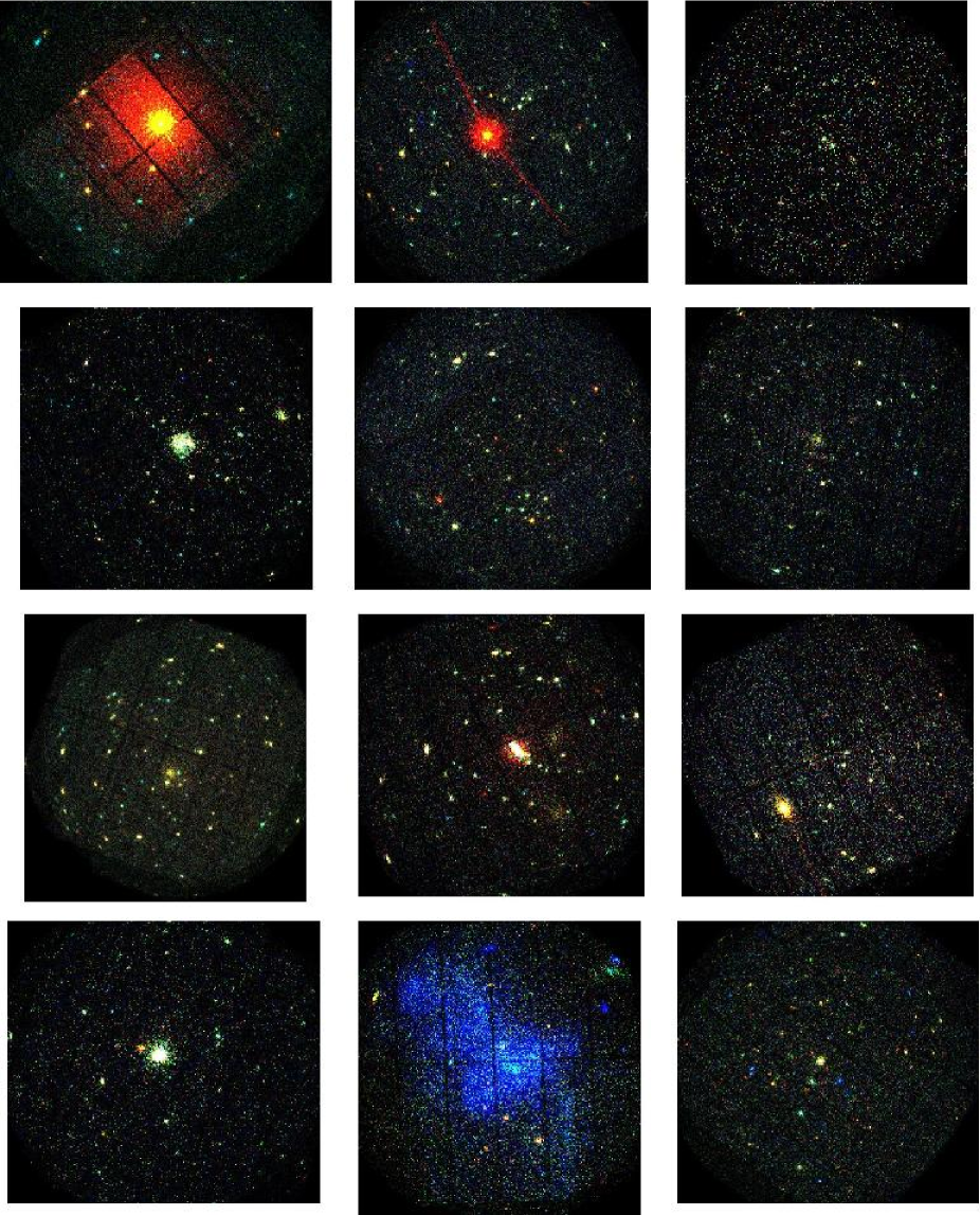
Figure 1: Color composite X-ray images for the 12 fields considered in this paper (XMM-01 to XMM-12 from top left to bottom right). The color images are composites within the so-called XID-band (0.5–4.5 keV). Red, green and blue channels comprise the energy ranges 0.5–1.0 keV, 1.0–2.0 keV, and 2.0–4.5 keV, respectively. Weighting of the sub-images was done in a manner that a typical extragalactic source with a power law spectrum with photon index 1.5 and absorption column density $N_{\mathrm{H}}=1\times 10^{20}$ cm^-2 would have equal photon numbers in all three bands. North is up and East to the left. The size of the images is typically $30\arcmin\times 30\arcmin$ but varies slightly with camera orientation.

The XMM-Newton data, both in raw and pipeline reduced form, are available through the XMM-Newton Science Archive. These data were used to create a wide range of products which include:

• Combined EPIC images in the XID-band 0.5–4.5 keV (FITS);

• Combined EPIC images in the total band 0.1–12 keV (FITS);

• Color images using three sub-bands, 0.5–1.0 keV (red), 1.0–2.0 keV (green), 2.0–4.5 keV (blue), in the XID-band (JPG).

As an illustration, Fig. 1 shows color composites of the final combined X-ray images for the 12 fields considered. Note that the X-ray images have a non-uniform exposure time over the field of view due to (1) the arrangements of the CCDs in the focal plane, which is different for the three cameras, and (2) the vignetting of the camera optics.

3 Optical observations

As mentioned earlier, the optical observations were carried out using WFI at the ESO/MPG-2.2m telescope in service mode. WFI is a focal reducer-type mosaic camera mounted at the Cassegrain focus of the telescope. The mosaic consists of $4\times 2$ CCD chips with $2048\times 4096$ pixels with a projected pixel size of $0\aas@@fstack{\prime\prime}{238}$, giving a FOV of $8\aas@@fstack{\prime}{12}\times 16\aas@@fstack{\prime}{25}$ for each individual chip. The chips are separated by gaps of $23\aas@@fstack{\prime\prime}{8}$ and $14\aas@@fstack{\prime\prime}{3}$ along the right ascension and declination direction, respectively. The full FOV of WFI is thus $34\arcmin\times 33\arcmin$ with a filling factor of $95.9$%.

The WFI data described in this paper are from the following two sources:

1. the ESO Large Programme 170.A-0789(A) (Principal Investigator: J. Krautter, as chair of the SWG) which has accumulated data from January 27, 2003 to March 24, 2004 at the time of writing.

2. the contributing programs 70.A-0529(A); 71.A-0110(A); 71.A-0110(B) with P. Schneider as the Principal Investigator, which have contributed data from October 14, 2002 to September 29, 2003

Observations were performed in the $B$-, $V$-, $R$-, and $I$-passbands. These were split into OBs consisting of a sequence of five (ten in the $I$-band) dithered sub-exposures with the typical exposure time given in Table 3. The table gives: in Col.1  the passband; in Col. 2 the filter id adopting the unique naming convention of the La Silla Science Operations Team; in Col. 3 the total exposure time in seconds; in Col. 4 the number of observing blocks (OBs) per field; and in Col. 5 the integration time of the individual sub-exposures in the OB. The dither pattern with a radius of 80″ was optimized for the best filling of the gaps. Filter curves can be found in Arnouts et al. (2001) and on the web page of the La Silla Science Operations Team.

Even though the nominal total survey exposure time for the $R$-band is 3500 s, the data contributed by the Bonn group provided additional exposures totaling 11 500 s each, spread over 4 OBs. For the same reason the $B$-band data for the field XMM-07 has a significantly larger exposure time than that given in Table 3 (see Table 9).

Table 3: Planned observing strategy for the XMM-Newton follow-up survey.

Passband	Filter	$T_{\mathrm{tot}}$ (s)	$N_{\mathrm{OB}}$	$T_{\mathrm{exp}}$ (s)
$B$	B/123_ESO879	1800	1	360
$V$	V/89_ESO843	4400	2	440
$R$	Rc/162_ESO844	3500	1	700
$I$	I/203_ESO879	9000	3	300

Service mode observing provides the option for constraints on e.g., seeing, transparency, and airmass to be specified in order to meet the requirements of the survey. The adopted constraints were: (1) dark sky with a fractional lunar illumination of less than $0.4$; (2) clear sky with no cirrus though not necessarily photometric; and (3) seeing $\leq 1\aas@@fstack{\prime\prime}2$. The $R$-band images of the contributing program were taken with a seeing constraint of $\lesssim 1\aas@@fstack{\prime\prime}0$ so that the data can be used for weak lensing studies.

The total integration time in some fields may be higher than the nominal one listed in Table 3 because unexpected variations in ambient conditions during the execution of an OB can cause, for instance, the seeing and transparency to exceed the originally imposed constraints. If this happens, the OB is normally executed again at a later time. In these cases the decision of using or not all the available data must be taken during the data reduction process. In the case of the present survey all available data were included in the reduction, which explains why in some cases the total integration time exceeds that originally planned.

This paper describes data accumulated prior to October 16, 2003, amounting to about 80 h on-target integration. The science data comprises 720 exposures split into 130 OBs. About 15% of the $B$-band and 85% of the $R$-band data are from the contributing programs.

4 Data reduction

The accumulated optical exposures were reduced and calibrated using the EIS Data Reduction System (da Costa et al., in preparation) and its associated image processing engine based on the C++ EIS/MVM library routines (Vandame 2004, Vandame et al., in preparation). This library incorporates routines from the multi-resolution visual model package (MVM) described in Bijaoui & Rué (1995) and Rué & Bijaoui (1997). It was developed by the EIS project to enable handling and reducing, using a single environment, the different observing strategies and the variety of single/multi-chip, optical/infrared cameras used by the different surveys carried out by the EIS team. The platform independent EIS/MVM image processing engine is publicly available and can be retrieved from the EIS web-pages.

The system automatically recognizes calibration and science exposures and treats them accordingly. For the reduction, frames are associated and grouped into Reduction Blocks (RBs) based on the frame type, spatial separation and time interval between consecutive frames. The end point of the reduction of an RB is a reduced image and an associated weight map describing the local variations of noise and exposure time in the reduced image. The data reduction algorithms are fully described in Vandame (2004).

In order to produce a reduced image, the individual exposures within an RB are: (1) normalized to 1 s integration; (2) astrometrically calibrated with the Guide Star Catalog version 2.2 (GSC-2.2) as reference catalog, using a second-order polynomial distortion model; (3) warped into a user-defined reference grid (pixel, projection and orientation), using a third-order Lanczos kernel; and (4) co-added only using the weight for discarding the flux contribution from masked pixels (e.g. satellite tracks automatically detected and masked using a Hough transformation), for which the pixel value is zero. Note that individual exposures in the RB are not scaled to the same flux level. This assumes that the time interval corresponding to an RB is small enough to neglect significant changes in airmass.

The 720 raw exposures were converted into 160 fully calibrated reduced images, of which 146 were released in the $B$- (36), $V$- (32), $R$- (43) and $I$- (35) passbands. Of the remaining 14, 10 were observed with wrong coordinates, three (XMM-05 ($R$), XMM-06 ($I$), XMM-12 ($V$)) were rejected after visual inspection and one (XMM-12) was discarded due to a very short integration time (73 s), associated to a failed OB. The number of reduced images (150) exceeds that of OBs (130) because the RBs were built by splitting the OBs in order to improve the cosmetic quality of the final stacked images, as discussed below.

The photometric calibration of the reduced images was obtained using the photometric pipeline integrated to the EIS data reduction system as described in more detail in Appendix B. In particular, the XMM-Newton survey data presented here were obtained in 41 different nights of which 37 included observations of standard star fields. For these 37 nights it was attempted to obtain photometric solutions. The four nights without standard star observations are: February 2, 3 and 4, 2003 (Public Survey); and November 8, 2002 (contributing program). For the nights with standard star observations, the number of measurements ranges from a few to over 300, covering from 1 to 3 Landolt fields.

Table 4: Summary of the number of nights with standard star observations and type of solution.

Passband	default	1-par	2-par	3-par	total
$B$	0	3	4	3	10
$V$	0	8	3	5	16
$R$	0	8	3	3	14
$I$	4	8	2	5	19

Table 4 summarizes the available photometric observations. The table lists: in Col. 1 the passband; in Col. 2–5 the number of nights assigned a default solution or a 1–3-parameter solution; and in Col. 6 the total number of nights with standard star observations. For three nights (March 26, 2003; April 2, 2003; August 6, 2003) the solutions obtained in the passbands $V$, $I$, $R$, respectively (either 2- or 3-parameter fits) deviate from the median by $-0.26$, $-0.5$, $-0.25$ mag. Of those, only the $I$-band zeropoint obtained for April 2, 2003 deviates by more than $3\sigma$ from the solutions obtained for other nights. Note that the type of solution obtained depends on the available airmass and color coverage, which in the case of the XMM-Newton survey depends on the calibration plan adopted by the La Silla Science Operations Team.

Because the EIS Survey System automatically carries out the photometric calibrations it is interesting to compare the solutions to those obtained by other means. Therefore, the automatically computed 3-parameter solutions of the EIS Survey System are compared with the best solution recently obtained by the La Silla Science Operations Team. The results of this comparison are presented in Table 5 which lists: in Col. 1 the passband; in Cols. 2–4 the mean offsets in zeropoint ($ZP$), extinction ($k$) and color term (color), respectively. The agreement of the solutions is excellent for all passbands. However, it is worth emphasizing that the periods of observations of standard stars available to the two teams do not coincide.

Table 5: Comparison between the EIS 3-parameter fit solutions and the Telescope Team’s best solution.

Passband	$\Delta ZP$	$\Delta k$	$\Delta$ color
$B$	$0.00$	$-0.03$	$-0.06$
$V$	$-0.05$	$0.00$	$-0.01$
$R$	$0.00$	$0.10$	$0.00$
$I$	$-0.04$	$0.05$	$-0.02$

Not surprisingly, larger offsets are found when 2- and 1-parameter fits are included, depending on the passband and estimator used to derive the estimates for extinction and color term. Finally, taking into consideration only 3-parameter fit solutions and after rejecting $3\sigma$ outliers one finds that the scatter of the zeropoints is $\lesssim 0.08$ mag. This number is still uncertain given the small number of 3-parameter fits currently available, especially in the $R$-band. The obtained scatter is a reasonable estimate for the current accuracy of the absolute photometric calibration of the XMM-Newton survey data.

There are two more points that should be considered in evaluating the accuracy of the photometric calibration of the present data. First, for detectors consisting of a mosaic of individual CCDs it is important to estimate and correct for possible chip-to-chip variations of the gain. For the present data these variations were estimated by comparing the median background values of sub-regions bordering adjacent CCDs. The determined variations were used to bring the gain to a common value for all CCDs in the mosaic. This was applied to both science and standard exposures. Second, it is also known that large-scale variations due to non-uniform illumination over the field of view of a wide-field camera exist. The significance of this effect is passband-dependent and becomes more pronounced with increasing distance from the optical axis (Manfroid & Selman 2001; Koch et al. 2004; Vandame et al. in preparation). Automated software to correct for this effect has been developed but due to time constraints it has not yet been applied to these data.

The final step of the data reduction process involves the assessment of the quality of the reduced images. Following visual inspection, each reduced image is graded, with the grades ranging from A (best) to D (worst). This grade refers only to the visual aspect of the data (e.g. background, cosmetics). Out of 150 reduced images covering (see Sect. 3) the selected XMM-Newton fields, 104 were graded A, 35 B, 7 C and 4 D. The images with grades C and D are listed in Table 6. The table, ordered by field and date, lists: in Col. 1 the field name; in Col. 2 the passband; in Col. 3 the civil date when the night started (YYYY-MM-DD); in Col. 4 the grade given by the visual inspection; and in Col. 5 the primary motive for the grade. It is important to emphasize that the reduced images must be graded, as grades are used in the preparation of the final image stacks. In particular, reduced images with grade D have no scientific value and were not released and were discarded in the stacking process discussed in the next section.

Table 6: Grades representing the visual assessment of the reduced images.

Field	Passband	Date	Grade	Comment
XMM-05	$R$	2002-10-14	D	strong stray light contamination
XMM-06	$I$	2003-01-29	D	inadequate fringing correction
XMM-12	$I$	2003-03-29	D	very short integration time
XMM-12	$V$	2003-09-27	D	out-of-focus
XMM-01	$V$	2003-02-01	C	strong shape distortions
XMM-07	$R$	2003-08-06	C	stray light contamination
XMM-10	$R$	2003-08-06	C	fringing
XMM-10	$R$	2003-09-23	C	fringing
XMM-10	$R$	2003-09-29	C	fringing
XMM-10	$R$	2003-09-29	C	fringing
XMM-10	$R$	2003-09-29	C	fringing

The success rate of the automatic reduction process is better than 95% and most of the lower grades are associated with observational problems rather than inadequate performance of the software operating in an un-supervised mode. An interesting point is that occasionally $R$-band images are also affected by fringing (see Table 6) – for instance, in the nights of August 6 and September 23 and 29, 2003, all from the contributing program. The night of August 6 is one of the nights for which the computed $R$-band zeropoint deviates from the median. This points out the need to consider applying fringing correction also in the $R$-band, at least in some cases. The $R$-band fringing problem accounts for five out of seven grade C images. The remaining cases are due to stray-light and strong shape distortions.

It should also be pointed out that the reduced images show a number of cosmic ray hits. This is because the construction of RBs was optimized for removing cosmic ray features in the final stacks using a thresholding technique. To this end the number of images in an RB was minimized for some field and filter combinations to have at least three reduced images entering the SB.

5 Final products

5.1 Images

The 146 reduced images with grades better than D were converted into 44 stacked (co-added) images using the EIS Data Reduction System. The system creates both a final stack, by co-adding different reduced images taken of the same field with the same filter (see Appendix C), and an associated product log with additional information about the stacking process and the final image. Note that all stacks (and catalogs) and their associated product logs are publicly available from the EIS survey release and ESO Science Archive Facility pages.

The final stacks are illustrated in Fig. 2 which shows cutouts from color composite images of the 12 fields. From this figure, one can easily see the broad variety of fields observed by this survey – dense stellar fields (XMM-01, XMM-02, XMM-12), sometimes with diffuse emission (XMM-11), extended objects (e.g. XMM-08), and empty fields at high galactic latitude (e.g. XMM-07). While the constraints imposed by the system normally lead to good results, visual inspection of the images after stacking revealed that at least in one case the final stacked image was significantly degraded by the inclusion of a reduced image (graded B) with high-amplitude noise. Therefore, this image was not included in the production of the corresponding stack. The reason for this problem is being investigated and may lead to the definition of additional constraints for the automatic rejection algorithm being currently used.

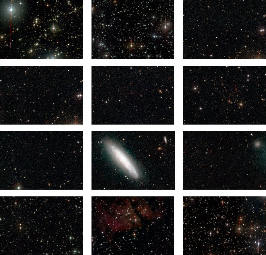
Figure 2: Above are cut-outs from color images of XMM-01 to XMM-12 (from top left to bottom right) to illustrate the wide variety of fields the pipeline can successfully handle. The color images are $BVR$ composite were $R$-band data is available, $BVI$ otherwise. The side length of the images displayed here is $7\aas@@fstack{\prime}{9}\times 5\aas@@fstack{\prime}{6}$. In these images North is up and East is to the left. These composite color images also demonstrate the accuracy of the astrometric calibration independently achieved in each passband.

Before being released the stacks were again examined by eye and graded. Out of 44 stacks, 33 were graded A, 10 B, and 1 C, with no grade D being assigned. In addition to the grade a comment may be associated and a list of all images with some comment can be found in the README file associated to this release in the EIS web-pages. The comments refer mostly to images with poor background subtraction either due to very bright stars (XMM-12) or extended, bright galaxies (XMM-08, XMM-09) in the field. It is important to emphasize that the reduction mode for these data was optimized for extragalactic, non-crowded fields, which is not optimal for some of these fields. Residual fringing is also observed in some stacks such as that of XMM-10 in the $R$-band and XMM-04, XMM-06 in the $I$-band.

As mentioned in the previous section, to improve the rejection of cosmic rays, the RBs were constructed so that in most cases the stack blocks (SB) consist of at least 3 reduced images as input. This allows for the use of a thresholding procedure, with the threshold set to $2.5\sigma$, to remove cosmic ray hits from the final stacked image. Even with this thresholding the stacks consisting of only three RBs (totaling 5 exposures), mostly $B$-band images, still show some cosmic ray hits. This happens primarily in the regions of the inter-chip gaps, where fewer images contribute to the final stack. Also, the automatic satellite track masking algorithm has proven to be efficient in removing both bright and faint tracks. The most extreme case is 3 satellite tracks of varying intensity in a single exposure. The regions affected by satellite tracks in the original images were flagged in the weight-map images and thus are properly removed from the stacked image. Naturally, in the regions where a satellite track was found in one of the contributing images the noise is slightly higher in the stacked image. This is also reflected in the final weight-map image.

The accuracy of the final photometric calibration of course depends on the accuracy of the photometric calibration of the reduced images which are used to produce the final co-added stacks and the number of independent photometric nights in which these were observed (see Table 7). The former depends not only on the quality of the night but also on the adopted calibration plan. To preview the quality of the photometric calibration, Table 7 provides information on the number of reduced images and number of independent nights for each passband and filter. The table gives for each field in: Col. 1 the field identification; Cols. 2–4 for each passband the number of reduced images with the number in parenthesis being the number of independent nights in which they were observed. Complementing this information Table 8 shows the best type of solution available for each field/filter combination. The table gives: in Col.1 the field name; in Cols. 2–5 the number of free parameters in the type of the best solution available for the passbands indicated. Solutions with more free parameters in general indicate better airmass and color coverage, yielding better photometric calibration. Examination of these two tables provide some insight into the quality of the photometric calibration of each final stack, as reported below.

Table 7: Summary of available data – number of reduced images and in parentheses number of independent nights – for each field and passband.

Field	$B$	$V$	$R$	$I$
XMM-01	3 (1)	3 (2)	3 (1)	3 (3)
XMM-02	3 (1)	3 (1)	3 (1)	3 (1)
XMM-03	3 (1)	3 (2)	5 (3)	3 (1)
XMM-04	3 (1)	3 (2)	4 (2)	3 (2)
XMM-05	3 (1)	3 (2)	5 (1)	3 (2)
XMM-06	3 (1)	3 (2)	6 (4)	3 (2)
XMM-07	3 (2)	3 (2)	6 (4)	3 (2)
XMM-08	3 (1)	3 (1)	—	3 (2)
XMM-09	3 (1)	3 (2)	—	3 (2)
XMM-10	3 (1)	—	5 (3)	—
XMM-11	3 (1)	3 (2)	3 (1)	5 (4)
XMM-12	3 (1)	2 (1)	3 (1)	3 (2)

Table 8: Type of best photometric solution available for each field.

Field	Default	1-par	2-par	3-par
XMM-01	$R$	$BV$	—	$I$
XMM-02	$RI$	$BV$	—	—
XMM-03	—	$I$	$R$	$BV$
XMM-04	—	$V$	—	$BRI$
XMM-05	—	$R$	$I$	$BV$
XMM-06	—	$V$	$BR$	$I$
XMM-07	—	$I$	$B$	$VR$
XMM-08	—	$V$	—	$BI$
XMM-09	—	—	$B$	$VI$
XMM-10	—	—	$B$	$R$
XMM-11	—	—	—	$BVRI$
XMM-12	—	$BR$	$V$	$I$

The main properties of the stacks produced for each field and filter are summarized in Table 9. The table gives: in Col. 1 the field identifier; in Col. 2 the passband; in Col. 3 the total integration time $T_{\mathrm{int}}$ in seconds, of the final stack; in Col. 4 the number of contributing reduced images or RBs; in Col. 5 the total number of science frames contributing to the final stack; in Cols. 6 and 7 the seeing in arcseconds and the point-spread function (PSF) anisotropy measured in the final stack; in Col. 8 the limiting magnitude, $m_{\mathrm{lim}}$, estimated for the final image stack for a 2″ aperture, $5\sigma$ detection limit in the AB system; in Col. 9 the grade assigned to the final image during visual inspection (ranging from A to D); in Col. 10 the fraction (in percentage) of observing time relative to that originally planned.

Table 9: Overview of the properties of the produced image stacks.

Field	Passband	$T_{\mathrm{int}}$	#RBs	#Exp.	Seeing	PSF rms	$m_{\mathrm{lim}}$	Grade	Completeness
		(s)			(arcsec)		(mag)		(%)
XMM-01	$B$	1800	3	5	1.19	0.056	24.94	A	100
XMM-01	$V$	6599	3	15	0.97	0.056	25.32	A	150
XMM-01	$R$	3500	3	5	0.82	0.074	23.97	B	100
XMM-01	$I$	8998	3	30	0.69	0.063	23.53	A	100
XMM-02	$B$	1800	3	5	1.17	0.051	24.51	A	100
XMM-02	$V$	4399	3	10	0.96	0.076	24.63	A	100
XMM-02	$R$	3500	3	5	0.64	0.087	24.69	A	100
XMM-02	$I$	5998	3	20	0.94	0.079	23.84	A	67
XMM-03	$B$	1800	3	5	1.01	0.031	25.44	A	100
XMM-03	$V$	4399	3	10	0.86	0.068	25.35	A	100
XMM-03	$R$	11 748	5	20	0.83	0.152	25.15	A	336
XMM-03	$I$	9297	3	31	0.96	0.061	24.39	A	103
XMM-04	$B$	1800	3	5	1.17	0.041	25.22	A	100
XMM-04	$V$	4399	3	10	1.07	0.050	25.05	A	100
XMM-04	$R$	11 748	4	20	0.76	0.069	25.57	A	336
XMM-04	$I$	8998	3	30	0.87	0.066	24.83	A	100
XMM-05	$B$	1800	3	5	1.24	0.076	25.18	A	100
XMM-05	$V$	4399	3	10	1.51	0.063	24.80	A	100
XMM-05	$R$	12 348	5	21	0.94	0.072	25.58	A	353
XMM-05	$I$	8998	3	30	1.09	0.056	24.58	A	100
XMM-06	$B$	1800	3	5	0.87	0.052	25.57	A	100
XMM-06	$V$	4399	3	10	0.73	0.039	25.43	A	100
XMM-06	$R$	14 998	6	25	0.85	0.060	24.54	A	429
XMM-06	$I$	8998	3	30	0.74	0.044	24.40	A	100
XMM-07	$B$	2699	2	8	1.24	0.035	25.55	A	150
XMM-07	$V$	4399	3	10	1.10	0.050	25.37	A	100
XMM-07	$R$	15 698	6	27	1.03	0.058	25.66	A	449
XMM-07	$I$	8998	3	30	0.95	0.048	24.96	A	100
XMM-08	$B$	1800	3	5	1.28	0.062	25.62	A	100
XMM-08	$V$	4399	3	10	1.03	0.082	24.93	A	100
XMM-08	$I$	8998	3	30	0.79	0.052	24.76	B	100
XMM-09	$B$	1800	3	5	0.94	0.045	24.59	B	100
XMM-09	$V$	4839	3	11	0.83	0.031	24.20	B	110
XMM-09	$I$	8998	3	30	0.72	0.038	23.81	B	100
XMM-10	$B$	1500	3	5	1.12	0.042	24.26	B	83
XMM-10	$R$	11 748	5	20	0.88	0.049	24.62	C	336
XMM-11	$B$	1800	3	5	1.09	0.058	25.25	A	100
XMM-11	$V$	4399	3	10	0.77	0.075	24.03	A	100
XMM-11	$R$	3500	3	5	0.60	0.090	23.10	A	100
XMM-11	$I$	12 297	5	41	0.77	0.087	22.64	A	137
XMM-12	$B$	1800	3	5	1.09	0.087	23.41	B	100
XMM-12	$V$	3519	2	8	0.79	0.085	23.48	B	80
XMM-12	$R$	4899	3	7	0.64	0.111	23.16	B	140
XMM-12	$I$	3599	3	12	1.21	0.093	22.01	B	40

This table shows that for most stacks the desired limiting magnitude was met in $V$ (24.92 mag) or even slightly exceeded in $B$ (25.20 mag). The $R$- and $I$-band images are slightly shallower than originally proposed with median limiting magnitudes of $24.66$ mag and $24.39$ mag. Still, when only the high-galactic latitude fields are included the median limiting magnitudes are fainter – 25.33 ($B$), 25.05 ($V$), 25.36 ($R$) and 24.58 ($I$) mag. All magnitudes are given in the AB system. The median seeing of all stacked images is $0\aas@@fstack{\prime\prime}94$ with the best and worst values being $0\aas@@fstack{\prime\prime}60$ and $1\aas@@fstack{\prime\prime}51$, respectively. This is significantly better than the seeing requirement of $1\aas@@fstack{\prime\prime}2$ specified for this survey.

Finally, the following remarks can be made concerning the image stacks and their calibration:

• XMM-01 ($R$) – The background subtraction near bright stars is poor. This field was observed as a single OB on February 3, 2003 for which no standard stars were observed. Since this is a galactic field there are no complementary observations from the contributing program, and therefore these observations cannot be calibrated.

• XMM-01 ($I$) – This field at low galactic latitude is very crowded and no acceptable fringing map could be produced from the science exposures in the field. The de-fringing was done with an external fringing map generated from science images taken on empty fields close in time to the XMM-01 $I$-band observations.

• XMM-02 ($R$) – The observations for this pointing and filter were done with one OB (5 exposures) on February 2, 2003 for which no standard stars observations were carried out.

• XMM-02 ($I$) – The observations for this pointing and filter were done with two OBs (10 exposures each) on February 2, 2003 for which no standard stars observations were carried out. Like for XMM-01 ($I$) an external fringing map was used.

• XMM-03 ($V$) – The $V$-band calibration on the night of March 26, 2003 yields a 3-parameter fit that deviates from the median of the solutions by roughly 0.26 mag (less than $3\sigma$).

• XMM-04 ($I$) – Low level fringing is still visible in the final stacked image.

• XMM-06 ($I$) – As in XMM-04, low level fringing is still visible in the final stack.

• XMM-07 ($B$) – From the three reduced images available only two were used for stacking because of the high amplitude of noise in one of them which greatly affected the final product.

• XMM-07 ($R$) – This field was observed in four nights (August 6, and September 23, 27, and 28, 2003) as part of the contributing program. For the night of August 6 a 3-parameter fit solution was obtained. However, this solution deviates by roughly 0.25 mag relative to the median of all $R$-band solutions.

• XMM-07 ($I$) – There is a visible stray light reflection at the lower right corner of the image.

• XMM-08 ($V$) – The bright central galaxy is larger than the dithering pattern, thus making it difficult to estimate the background in its neighborhood. As a consequence the background subtraction procedure does not work properly.

• XMM-08 ($I$) – The comments about the background subtraction for the $V$-band image also apply to the $I$-band. This field was observed using 3 OBs (which in this case also correspond to 3 RBs) on two nights (March 30, 2003, one OB and April 2, 2003, two OBs). On the night of April 2 a 3-parameter solution was obtained for which the ZP determined deviates significantly (more than $3\sigma$) from the median of all solutions, even though the conditions of the night seem to have been adequate. The reason for this poor solution is at present unknown. Poor fringing correction is a possibility but needs to be confirmed. The zeropoint for the two reduced images taken in this night has been replaced by a default value.

• XMM-09 ($BVI$) – The preceding comment about background subtraction (see XMM-08) can be repeated here for the large galaxy in the North-West corner of the image. The background subtraction procedure fails, creating a strong variation around the galaxy.

• XMM-10 ($B$): This stack has a shorter exposure time than the others released, leading to higher background noise.

• XMM-10 ($R$) – This field was observed in the nights of August 6, and September 23 and 29, 2003 as part of contributing program. As in case of XMM-07 the solution for August 6 deviates somewhat from the median.

• XMM-11 ($V$) – The same comments as for the photometric calibration of XMM-03 ($V$) apply to this image.

• XMM-11 ($I$) – Like for XMM-01 ($I$) an external fringing map was used.

• XMM-12 ($BR$) – The background subtraction near bright stars is poor.

• XMM-12 ($V$) – The preceding comment about background subtraction also applies to this image. In addition the comment about the photometric calibration of XMM-03 ($V$-band) also applies to this image.

• XMM-12 ($I$) – The comment about background subtraction also applies to the $I$-band image. Like for XMM-01 ($I$) an external fringing map was used.

Some improvements in the image quality may be possible in the future by adopting a different observing strategy such as larger dithering patterns to deal with more extended objects or shorter exposure times to minimize the impact of fringing.

5.2 Catalogs

For the 8 fields located at high-galactic latitudes with $|b|>30^{\circ}$, a total of 28 catalogs were produced (not all fields were observed in all filters, see Table 7). Catalogs for the remaining low-galactic latitude fields were not produced since these are crowded stellar fields for which SExtractor alone is not well suited. As in the case of the Pre-FLAMES survey (Zaggia et al., in preparation), it is preferable to use a PSF fitting algorithm such as DAOPHOT (Stetson 1987). Details about the catalog production pipeline available in the EIS data reduction system are presented in Appendix D.

As mentioned earlier, the fields considered here cover a range of galactic latitudes of varying density of objects, in some cases with bright point and extended sources in the field. In this sense this survey is a useful benchmark to evaluate the performance of the procedures adopted for the un-supervised extraction of sources and the production of science-grade catalogs. This also required carrying out tests to fine-tune the choice of input parameters to provide the best possible compromise. Still, it should be emphasized that the catalogs produced are in some sense general-purpose catalogs. Specific science goals may require other choices of software (e.g. DAOPHOT, IMCAT) and/or input parameters.

A key issue in the creation of catalogs is to minimize the number of spurious detections and in general, the adopted extraction parameters work well. However, there are unavoidable situations where this is not the case. Among these are: (1) the presence of ghost images near bright stars. Their location and size vary with position and magnitude making it difficult to deal with them in an automatic way; (2) the presence of bright galaxies because the algorithm for automatic masking does not work well in this case; (3) residual fringing in the image; (4) the presence of stray light, in particular, associated with bright objects just outside the observed field; (5) when the image is slightly rotated, the trimming procedure does not trim the corners of the image correctly, leading to the inclusion of regions with a low $S/N$. In these corners many spuriously detected objects are not flagged as such. The XMM-Newton fields are a good showcase for these various situations.

Another important issue to consider is the choice of the parameter that controls the deblending of sources. Experience shows that the effects of deblending depend on the type of field being considered (e.g. empty or crowded fields, extended object, etc.) and vary across the image. Some tests were carried out but further analysis of this topic may be required.

A number of tests have also been carried out to find an adequate compromise for the scaling factor used in the calculation of the size of the automatic masks (see Appendix D) which depends on the passband and the magnitude of the object. While the current masking procedure generally works well, the optimal scaling will require further investigation. It is also clear that for precision work, such as e.g. lensing studies, additional masking by hand is unavoidable. It should also be mentioned that occasionally the masking of saturated stars fails. This occurs in five out of the 28 catalogs released and only for $\sim$10% of the saturated stars in them. These cases are likely to be of stars just barely saturated, at the limit of the settings for automatic masking.

Bearing these points in mind, the following comments can be made regarding some of the released catalogs:

• XMM-03 ($B$) – The automatic masking misses a few saturated stars.

• XMM-06 ($B$) – Due to a small rotation of the image of a few degrees the trimming frame does not mask the borders completely.

• XMM-06 ($V$) – The deblending near bright galaxies is insufficient. Deblending near bright stars is too strong.

• XMM-06 ($R$) – As in the $V$-band image the deblending near bright galaxies is insufficient.

• XMM-06 ($I$) – As in the $V$-band image the deblending near bright galaxies is insufficient. Spurious object detections are caused by reflection features of bright stars and stray light reflections.

• XMM-07 ($B$) – Spurious objects in the corners are caused by insufficient trimming.

• XMM-08 ($B$) – Masks are missing for a number of saturated stars. XMM-08 contains an extended, bright galaxy (NGC 4666) at the center of the image, plus a companion galaxy located South-East of it. The presence of these galaxies leads to a large number of spurious object detections in their surroundings in all bands.

• XMM-08 ($VRI$) – See the comments about spurious object detections for XMM-08 $B$-band.

• XMM-09 ($B$) – Cosmic rays are misidentified as real objects. The very bright galaxy located at the North-West of the image leads to the detection of a large number of spurious objects extending over a large area ($10\arcmin\times 10\arcmin$) in all bands. Even though the galaxy has been automatically masked, the affected area is much larger than that predicted by the algorithm, which is optimized for stars. Thus, additional masking by hand would be required.

• XMM-09 ($VI$) – See the comments about spurious object detections for XMM-09 $B$-band.

• XMM-10 ($R$) – The stacked image was graded C because of fringing. The fringing pattern causes a high number of spurious object detections along the fringing pattern, leading to a catalog with no scientific value. This catalog is released exclusively as an illustration.

6 Discussion

6.1 Comparison of counts and colors

A key element in public surveys is to provide potential users with information regarding the quality of the products released. To this end a number of checks of the data are carried out and several diagnostic plots summarizing the results are automatically produced by the EIS Survey System. They are an integral part of the product logs available from the survey release page. Due to the large number of plots produced in the verification process these are not reproduced here. Instead a small set illustrating the results are presented.

A relatively simple statistics that can be used to check the catalogs and the star/galaxy separation criteria is to compare the star and galaxy number counts derived from the data to that of other authors and/or to model predictions. As an example, Fig. 3 shows the galaxy counts in different observed passbands for the field XMM-07. Here objects with CLASS_STAR$<0.95$ or fainter than the object classification limit were used to create the sample of galaxies. Note that the number counts shown in the figure take into account the effective area of the catalog, which is available in its FIELDS table (see Appendix D). As can be seen, the computed counts are consistent with those obtained by previous authors for all passbands (Arnouts et al. 2001; Metcalfe et al. 2001).

Figure 3: Galaxy number counts for the XMM-07 field for the different passbands as indicated in each panel. Full circles represent EIS data points, open triangles Metcalfe et al. (2001), open squares Arnouts et al. (2001).

A complementary test is to compare the stellar counts to those predicted by models, such as the galactic model of Girardi et al. (2005, and references therein). Generally, the agreement of model predictions is excellent for $B$- and $V$-band catalogs, becoming gradually worse for $R$- and especially in $I$-band, near the classification limit, with the counts falling below model predictions (e.g. XMM-09 $I$-band). Note, however, that plots of CLASS_STAR versus magnitude show a less well defined stellar locus for these bands. It is thus reasonable to assume that the observed differences between catalogs and model predictions are due to misclassification of stars as galaxies. Alternatively, these may also reflect short-comings in the model adopted. However, a detailed discussion of this issue is beyond the scope of the present paper.

While useful to detect gross errors, number counts are not sufficiently sensitive to identify more subtle differences. The comparison of expected colors of stars with theoretical models provides a better test of the accuracy of the photometric calibration in the different bands. Using color transformations computed in the same way as in Girardi et al. (2002), the theoretical colors of stars can be obtained. Such comparisons were made for all five fields with data in four passbands. The results for two cases, XMM-06 and XMM-07 are illustrated in Figs. 4 and 5, respectively, which show $(B-V)\times(V-I)$ and $(V-R)\times(R-I)$ diagrams. For XMM-06 the data are in excellent agreement with the colors of stars predicted by the theoretical model, with only a small ($\lesssim 0.05$ mag) offset in $R-I$, indicating a good calibration. On the other hand, for XMM-07, one observes a significant offset ($\sim 0.2$ mag) in $B-V$. This field was chosen because it exemplifies the worst offset observed relative to the theoretical models. Since this offset is only visible in the $(B-V)\times(V-I)$ diagram, it suggests a problem in the $B$-band data. Data for this field/filter combination comes from two nights 2003-06-30 and 2003-08-06. Closer inspection of the observations in the night of 2003-06-30 show that: (1) the standard stars observations span only 2 hours in the middle of the night; (2) the photometric zeropoint derived using the available measurements (24.59 mag) is reasonably close ($\sim 1\sigma$) to the median value of the long-term trend (24.71 mag); (3) the $B$ exposures were taken close to sunrise; and (4) there was a significant increase in the amplitude of the DIMM seeing at the time the XMM-07 exposures under consideration were taken. For the night of 2003-08-06 standards cover a much larger time interval, yielding a zeropoint of 24.82 mag with comparable difference relative to the long-term median value for this filter as given above. The results suggest that the observed problem is not related to the calibration of the night, as will be seen below.

6.2 Comparison with other reductions

Table 10: Summary of the astrometric and photometric comparison. All differences were computed EIS$-$GaBoDS.

Field	Target	Passband	$\Delta\alpha\cos(\delta)$	$\Delta\delta$	$\Delta m$
			(arcsec)	(arcsec)	(mag)
XMM-03	HE 1104$-$1805	$B$	$0.02\pm 0.04$	$-0.01\pm 0.03$	$0.13\pm 0.02$
XMM-03	HE 1104$-$1805	$R$	$0.02\pm 0.05$	$-0.01\pm 0.05$	$0.01\pm 0.04$
XMM-04	MS 1054.4$-$0321	$B$	$0.00\pm 0.05$	$0.00\pm 0.05$	$0.12\pm 0.04$
XMM-04	MS 1054.4$-$0321	$V$	$0.02\pm 0.05$	$-0.00\pm 0.05$	$0.00\pm 0.04$
XMM-04	MS 1054.4$-$0321	$R$	$0.03\pm 0.06$	$0.00\pm 0.06$	$0.00\pm 0.03$
XMM-05	BPM 16274	$B$	$0.00\pm 0.06$	$-0.01\pm 0.06$	$0.05\pm 0.04$
XMM-05	BPM 16274	$R$	$0.03\pm 0.09$	$-0.01\pm 0.09$	$0.18\pm 0.04$
XMM-06	RX J0505.3$-$2849	$B$	$0.02\pm 0.04$	$0.00\pm 0.04$	$0.00\pm 0.02$
XMM-06	RX J0505.3$-$2849	$V$	$0.02\pm 0.04$	$-0.01\pm 0.04$	$-0.04\pm 0.04$
XMM-06	RX J0505.3$-$2849	$R$	$0.01\pm 0.03$	$0.01\pm 0.04$	$0.05\pm 0.03$
XMM-07	LBQS 2212$-$1759	$B$	$0.02\pm 0.06$	$-0.02\pm 0.06$	$0.34\pm 0.04$
XMM-08	NGC 4666	$B$	$0.00\pm 0.06$	$-0.01\pm 0.05$	$0.00\pm 0.03$
XMM-08	NGC 4666	$V$	$0.00\pm 0.06$	$-0.01\pm 0.05$	$-0.01\pm 0.03$
XMM-09	QSO B1246$-$057	$B$	$0.02\pm 0.06$	$-0.01\pm 0.05$	$0.02\pm 0.02$
XMM-10	PB 5062	$B$	$-0.03\pm 0.05$	$-0.01\pm 0.07$	$0.05\pm 0.02$

As shown above, comparison of different statistics, based on the sources extracted from the final image stacks, to those of other authors and to model predictions provide an internal means to assess the quality of the data products. However, in the particular case of this survey one can also benefit from the fact that about one third of the accumulated data has been independently reduced by the Bonn group in charge of the contributing program (Sect. 3). The images in common are used in this section to make a direct comparison of the astrometric and photometric calibrations. In their reduction, the Bonn group used their “Garching-Bonn Deep Survey” (GaBoDS) pipeline (Erben et al. 2005).

A total of 15 stacked images in the $B$-, $V$-, and $R$-bands were produced and compared to those produced by the EIS/MVM pipeline. The astrometric calibration was done using the GSC-2.2 catalog, the same as that of the EIS reduction. In contrast to the reductions carried out by the EIS system, images were photometrically calibrated using the measurements of standard stars compiled by Stetson (2000). The type of solution (number of free parameters of a linear fit) for a night was decided on a case by case basis after visual inspection of the linear fits.

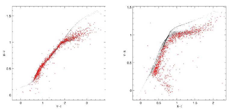
Figure 4: $BVI$ (left panel) and $VRI$ (right panel) color-color plot for stars objects in the XMM-06 field (large dots) and that obtained using theoretical models (small dots).

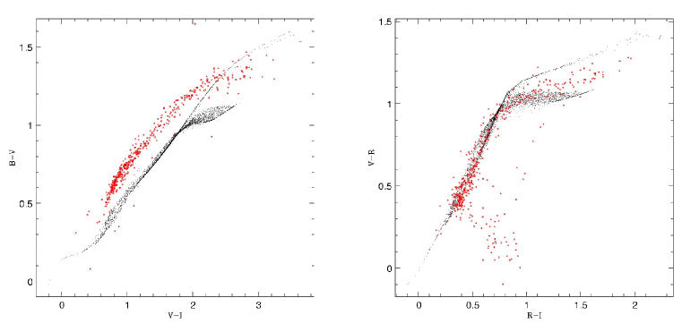
Figure 5: Same as Fig. 4 for XMM-07.

To carry out the comparison of the data products, catalogs were produced from the EIS and GaBoDS images using the same extraction parameters. These catalogs were associated with each other to produce a merged catalog for each field and passband. The results of this comparison for all the available images in common are presented in Table 10. The table gives: in Col. 1 the field name; in Col. 2 the original target name; in Cols. 3 and 4 the mean offset and standard deviation in right ascension and declination in arcseconds; in Col. 5 the mean and standard deviation of the magnitude differences as measured within an aperture of 3″. The mean and standard deviation of the magnitude differences were determined in the interval $17<m<21$. This range was chosen to avoid saturated objects at the bright end and to limit the comparison to objects whose estimated error in magnitude is smaller than about $0.01$ mag at the faint end. An iterative $5\sigma$ rejection, which allowed rejected points to re-enter if they are compatible with later determinations of the mean and variance, was employed to ignore obvious outliers in the computation of the mean and the standard deviation.

Fig. 6 illustrates the results obtained from the comparison of the position of sources extracted from images produced by the two pipelines for the particular case of XMM-06 in $R$-band. From the figure one can see that the positions of the sources agree remarkably well. In fact, as summarized in Table 10, the typical mean deviation is $\sim 20$ mas with a standard deviation of $\sim 50$ mas, confirming the excellent agreement in the external (absolute) astrometric calibration to be distinguished from the internal calibration discussed later.

Fig. 7 shows a plot of the magnitude differences measured on the GaBoDS $R$-band image of the field MS 1054.4$-$0321 (XMM-04) versus the magnitudes measured on the corresponding EIS image. This field shows that the photometry of both reductions agree remarkably well. The measured scatter of the magnitude differences is small ($\sim 0.03$ mag) for this as well as for most other fields. This result indicates that the internal procedures used by the two pipelines to estimate chip-to-chip variations are consistent. Moreover, inspection of the last column of Table 10 shows that for 11 out of 15 cases the mean offsets are $\lesssim$0.05 mag. This is reassuring for both pipelines considering all the differences involved in the process, which include differences in the routines, procedures and the standard stars used. It is important to emphasize that differences in the computed zeropoint of the photometric solutions are $\lesssim$ 0.08 mag, even for the cases with the largest differences such as XMM-05 ($R$) and XMM-07 ($B$). The value of 0.08 mag is consistent with the scatter measured from the long-term trend shown by the zeropoints computed over a large time interval, as presented in the EIS release of WFI photometric solutions, thus representing the uncertainty in the photometric calibration. Therefore, the offsets reported in the table cannot be explained by differences in the photometric calibration alone. This point is investigated in more detail for XMM-05 $R$-band and XMM-07 $B$-band.

Figure 6: Comparison of astrometry for the $R$-band image of XMM-06 (RX J0505.3$-$2849), selected to represent a typical case. The offsets are computed EIS$-$GaBoDS. The dashed lines are centered on $(0,0)$, while the solid lines denote the actual barycenter of the points.

All $R$-band images for XMM-05 were taken in one night and the photometric solutions determined by both teams agree very well. While the source of the discrepancy has not yet been identified, the stellar locus in the $(B-V)\times(V-I)$ and $(V-R)\times(R-I)$ diagrams based on the source catalog extracted from the EIS images yield results which are consistent with model predictions, suggesting that the problem may lie in the Bonn reductions. On the other hand, the large offset (0.34 mag) between the $B$-band observations of the field XMM-07 is most likely caused by the data taken in the night 2003-06-30. While the standard star observations in this night suggest relatively good photometric conditions, the available measurements span only about 2 hours in the middle of the night, while the science exposures were taken at the very end of the night. Inspection of the ambient condition shows a rapid increase in the amplitude of the DIMM seeing which could be related to a localized variation in the transparency. In fact, the Bonn pipeline, which monitors the relative differences in magnitude for objects extracted from different exposures in an OB, finds strong flux variations that could be caused by changes in the sky transparency or by the twilight at sunrise. The latter could also account for the fact that these observations were later repeated in August of that year. The important point is that the Bonn group discarded the calibration of the frames taken in 2003-06-30, while the automatic procedure adopted by EIS did not.

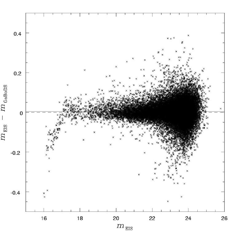
Figure 7: Comparison of aperture magnitudes (3″ aperture) measured on the $R$-band image of the field XMM-04 (MS 1054.4$-$0321). The dashed line is at a magnitude difference of 0, while the solid line denotes the actual offset between the EIS and the GaBoDS reduction. The difference at the bright end is caused by different treatments of saturated objects in both pipelines.

Figure 8: Stellar PSF pattern in the $R$-band images of the field MS 1054.4$-$0321 in the EIS reduction (left panel) and the GaBoDS reduction (right panel). The encircled stick in the left panel denotes an ellipticity of $\varepsilon=0.01$. Both plots have the same scale.

In addition to evaluating the accuracy of the image registration and photometric calibration, the independent reductions also offer the possibility to evaluate the shape of the images. To this end the PSF of bright, non-saturated stars on the $R$-band images for XMM-04 (MS 1054.4$-$0321) and XMM-06 (RX J0505.3$-$2849) were measured and compared. These are the only two cases in which the final stacked images were produced by using exactly the same reduced images. This is caused by the differences in the criteria adopted in building the SBs. In the case of XMM-06, one finds that the size and pattern of the PSF are in good agreement and both reductions yield a smooth PSF with no obvious effects of chip boundaries over the whole field. The situation is different for XMM-04 as can be seen in Fig. 8, which shows a map of the PSF distortion obtained by the EIS (left panel) and Bonn (right panel) groups. While the overall pattern of distortion is similar, the amplitude of the PSF distortion of the EIS reduction is significantly larger and exhibits jumps across chip borders. Although the effect is small in absolute terms, it should be taken into account for applications relying on accurate shape measurements. The reason for these differences is likely due to the fact that the astrometric calibration in the EIS pipeline is done for each chip relative to an absolute external reference, without using the additional constraint that the chips are rigidly mounted to form a mosaic. By neglecting this constraint, the solution for each chip in the mosaic may vary slightly depending on the dithered exposure being considered and the density and spatial distribution of the reference stars in and around the field of interest. Since the accuracy of the GSC-2.2 of $250$ mas is approximately equal to the pixel size of WFI of $0\aas@@fstack{\prime\prime}{238}$, in addition to the absolute calibration of the image centroid, finding an internal relative astrometric solution further ensures that images in different dithered exposures map more precisely onto each other during co-addition. Imperfections in the internal relative astrometry result in objects not being matched exactly onto each other, thereby degrading the PSF of the co-added image.

6.3 X-ray/optical correlation

As pointed out in the introduction, the ultimate goal of this optical survey has been to provide catalogs from which one can identify and characterize the optical properties of X-ray sources detected with deep XMM-Newton exposures.

X-ray source lists for the high-galactic latitude fields were produced by the AIP-node of the SSC. These are based on pipeline processed event lists which were obtained with the latest official version of the Software Analysis System (SAS-V6.1). In its current version this SAS-based pipeline does not work with stacked images.

Source detection was performed as a three-stage process using eboxdetect in local and in map mode followed by a multi-PSF fit with emldetect for all sources present in the initial source lists. The multi-PSF fit invoked here works on 15 input images, i.e. 5 per EPIC camera. The five energy bands used per camera cover the ranges: (1) 0.1–0.5 keV; (2) 0.5–1.0 keV; (3) 1.0–2.0 keV; (4) 2.0–4.5 keV; and (5) 4.5–12.0 keV.

The SAS task eposcorr was applied to the X-ray source list. Eposcorr correlates the X-ray source positions with the positions from an optical source catalog, in this case the EIS catalog, to correct the X-ray positions, assuming that the true counterparts are contained in the reference catalogue.

The source detection scheme used here is very similar to the pipeline implemented for the production of the second XMM-Newton catalog of X-ray sources to be published by the XMM-Newton-SSC later in 2005 (Watson et al., in preparation). This approach is superior to that used for the creation of source lists which are currently stored in the XMM-Newton Science Archive since it makes use of X-ray photons from all cameras simultaneously. It also distinguishes between point-like and extended X-ray sources. In this paper we only consider point-like sources. Extended sources at high galactic latitudes are almost exclusively galaxy clusters and cannot be matched with individual objects in the optical catalogs. Examining their properties is beyond the scope of this work.

In carrying out the matching between the XMM-Newton source lists and those extracted from the optical images, it is important to note that the X-ray images lie fully within the FOV of the WFI images. Hence an optical counterpart can be potentially found for any of the X-ray sources.

From the high-galactic latitudes there are 3 fields with more than one observation. However, for XMM-05 only the two available observations with good time $t>10$ ks were considered. One of them had technical problems that prevented it from being used for catalog extraction. For XMM-09 the source list created contained many spurious sources due to remaining calibration uncertainties in the pipeline processed images and was not considered further. Figures showing the results of the source detection process with all sources indicated on an image in TIFF format, the composite X-ray images, and the source lists can be found on the web-page of the AIP-SSC-node. Below these source lists are used to identify their optical counterparts.

The extraction yields 995 point-like X-ray sources of which 742 are unique. The difference between these two numbers reflects differences in the three independent source lists extracted from the field XMM-07. The mean flux of the 742 unique X-ray sources is $F_{\mathrm{mean}}(0.5-2.0\,\mathrm{keV})=8.5\times 10^{-15}$ erg cm^-2 s^-1, the median flux in this band is $F_{\mathrm{med}}(0.5-2.0\,\mathrm{keV})=3.7\times 10^{-15}$ erg cm^-2 s^-1. Sources with $F(0.5-2.0\,\mathrm{keV})=4\times 10^{-15}$ erg cm^-2 s^-1 are detected already with an exposure time of 5 ks, while the limiting flux in the EIS-XMM fields at the deepest exposure levels is $F_{\mathrm{lim}}\simeq 3\times 10^{-16}$ erg cm^-2 s^-1.

Table 11: Contents of X-ray source lists for high-latitude XMM-EIS fields.

Field	Obs. ID	$N_{\mathrm{s}}$	Passband	$N_{\mathrm{m}}$	$N_{\mathrm{1}}$	$(N_{\mathrm{1}}/N_{\mathrm{s}})(\%)$	$N_{\mathrm{all}}$	$N_{\mathrm{1,all}}$	$B$	$V$	$I$	$BV$	$BI$	$BVI$
(1)	(2)	(3)	(4)	(5)	(6)	(7)	(8)	(9)	(10)	(11)	(12)	(13)	(14)	(15)
XMM-03	0112630101	69	$R$	92	61	88	62	47	1	1	1	0	0	0
		69		36	35	51	27	27	0	0	0	0	0	0
XMM-04	0094800101	101	$R$	156	91	90	84	68	0	0	1	1	0	0
		101		74	73	72	57	57	0	1	1	0	0	1
XMM-05	0125320401	89	$R$	130	79	89	52	42	1	0	2	0	0	0
		89		59	57	64	37	37	1	0	2	1	0	0
XMM-06	0111160201	110	$R$	173	101	92	105	79	1	1	0	0	0	0
		110		76	72	65	61	58	3	0	1	0	0	0
XMM-07	0106660101	144	$R$	191	119	83	84	66	3	0	2	1	0	2
		144		82	81	56	52	52	2	2	1	1	0	1
XMM-07	0106660201	110	$R$	134	91	83	65	53	3	0	2	1	0	2
		110		62	61	56	39	39	1	0	0	2	1	0
XMM-07	0106660601	162	$R$	211	139	86	93	76	1	0	1	2	0	0
		162		100	98	60	59	59	1	1	1	2	0	1
XMM-08	0110980201	123	$I$	130	97	79	82	70	1	0	—	0	—	—
		123		73	73	59	58	58	0	2	—	1	—	—
XMM-10	0012440301	88	$R$	113	76	86	50	46	1	—	—	—	—	—
		88		57	56	64	35	34	3	—	—	—	—	—

Nearly all the X-ray source lists were matched to catalogs extracted from the $R$-band images, with the exception of field XMM-08, which was correlated with the $I$-band. Two search radii, 2″ and 5″, were used. The larger value reflects the typical statistical error in X-ray source position determination (typically in the range $\sim 0.5\arcsec\text{--}2\arcsec$), coupled with an additional systematic error component ($\sim 1\arcsec$) in the attitude of the spacecraft. Hence, a matching radius of 5″ corresponds to roughly a $2\text{--}3\sigma$ uncertainty for most of the sources. The smaller correlation radius is justified by the distribution of the positional accuracy of the X-ray sources, which peaks at $\sim 1\aas@@fstack{\prime\prime}3$. It extends up to 3″ with the majority of sources (92%) being within 2″.

The results of X-ray source extraction and their cross-identification with their optical counterparts for 7 high-galactic latitude fields (9 observations) are summarized in Table 11. For each field two rows are given: the first row refers to the matching done with a 5″ search radius, in the second row the numbers for the smaller 2″ search radius are reported. The table lists: in Col. 1 the field name; in Col. 2 the Obs. ID of the XMM-Newton observation; in Col. 3 the number of detected X-ray point sources with a likelihood of existence larger than detml = 6, $N_{\mathrm{s}}$; in Col. 4 the passband of the catalog used as the optical reference for matching; in Col. 5 the number of matches, $N_{\mathrm{m}}$ within 5″ (2″); in Col. 6 the number of X-ray sources with at least one match $N_{\mathrm{1}}$. In the case of multiple matches the $m=1$ sources refer to the closest matching optical source; in Col. 7 the identification rate $N_{\mathrm{1}}/N_{\mathrm{s}}$; in Col. 8, the number of X-ray sources, which have at least one counterpart in the optical reference catalog, and are also detected in all other available optical passbands. This is a subset of the objects listed in Col. 5; in Col. 9, the same as in the previous column but for the $m=1$ optical counterparts, $N_{\mathrm{1,all}}$, which is a subset of the objects listed in Col. 6; finally, in Col. 10–15 the number of optical counterparts in other passbands, which are not detected in the reference catalog. In Col. 13–15 $BV$, $BI$ and $BVI$ refer to objects which are simultaneously detected in the respective passband but do not correspond to matches of X-ray sources with the reference catalog. Because we only list objects without match in the reference catalog the number of objects reported in Col. 10–15 is in some cases higher in the second row than in the first row. These are X-ray sources with matches in $B$-, $V$-, or $I$-band within a circle of 2″ having matches in the reference catalog only in the larger 5″ search radius.

The results of the X-ray/optical cross-correlation for all fields with available $R$-band catalogs (619 unique sources) are displayed in Fig. 9. The figure shows: (top left) the multiplicity function; (top right) the cumulative fraction of X-ray sources with optical counterparts in a 5″search radius (dashed line) and a 2″search radius (straight line); (bottom left) the distribution of the positional offsets between X-ray and optical sources; and (bottom right) the corresponding scatter plot in the $\alpha\leavevmode\nobreak\ \times\leavevmode\nobreak\ \delta$ plane. Note that in three panels all $m=1$ matches are represented by filled histograms and/or larger symbols.

Inspection of Fig. 9 shows that: (1) about 87% (61%) of the X-ray point sources have at least one optical counterpart within the search radius of 5″ (2″) down to $R\sim 25$ mag, and very few sources have more than 3 matches. In only very few cases one finds up to five associated optical sources, i.e. potential physical counterparts; (2) only about 15% of the X-ray sources have counterparts down to the Digital Sky Survey magnitude limit ($R\sim 20.5$), underscoring the need for dedicated optical imaging in order to identify the X-ray source population; (3) the distribution of the X-ray/optical positional offset peaks at around 1″ for the sources with $m=1$. The $m=1$ matches are well concentrated within a circle of 2″. The distribution is almost flat if all associations are considered. This underlines that the true physical counterparts to the X-ray sources will be found predominantly among the $m=1$ sources, i.e. the nearest and in most cases single associated optical sources; (4) the positional differences between X-ray and optical coordinates seem to be randomly distributed.

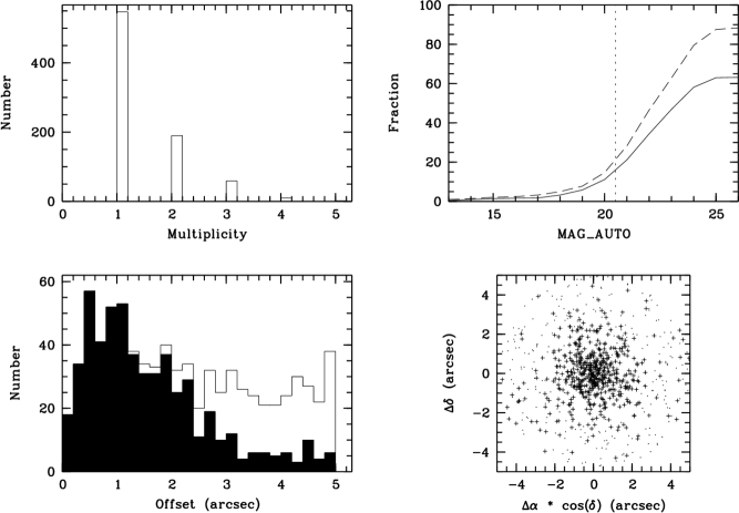
Figure 9: X-ray/optical $R$-band positional correlation. (top left) number of correlated optical sources to X-ray sources within 5″; (top right) cumulative fraction of X-ray sources with optical counterparts in the $R$-band catalog. The dashed line is for the 5″search radius, the straight line for the 2″search radius. The vertical short-dashed line denotes the approximate limit of the DSS; (bottom left) distribution of X-ray minus optical positional offset of all and $m=1$ sources; (bottom right) distribution of positional offsets in the right ascension – declination plane.

The statement that the additional correlations found within the greater search radius are chance alignments is strengthened by an estimate of the number of random matches between X-ray and optical sources. Using an average of 110 X-ray sources per field we can compute the total area covered by the search circles with 5″(2″) radius. Multiplying this with the typical number density of sources in the optical catalogs (30 arcmin^-2) we estimate 70 (12) random matches for an average field. The number of random matches within the smaller correlation radius is well below the observed number of optical/X-ray counterparts.

In addition, from this preliminary analysis the following conclusions can be drawn: (1) about 39% of the X-ray sources have no associated optical source within 2″. This optical identification completeness is comparable with that found by Eckart et al. (2005) in a similar study of X-ray source samples, but there may also be small contributions from sources with larger offsets than allowed by the adopted search radius, contamination by spurious X-ray sources, and random matches with the optical catalogs; (2) over 50% of the $m=1$ sources are detected in all the other bands available, within 1″; (3) correlations which occur at search radii greater than 2″ are most likely random correlations with the comparably dense optical catalogs; (4) all sources which are detected in $RI$ are also detected in $BV$, indicating that the optical counterparts of the X-ray sources are not excessively red or, even if they are red, the blue images are sufficiently deep to detect them; (5) the small number of X-ray sources matched with objects in the $B$- and $V$-band catalogs without matches in the $R$-band catalog suggests that we are also not dealing with excessively blue objects. Figure 10 shows color-color diagrams for the field XMM-06 for stars and galaxies in the field and compares it with the optical colors of X-ray sources matching objects in the optical catalogs. Stars and galaxies were selected using the SExtractor CLASS_STAR classifier with the cuts made at $\mathrm{CLASS\_STAR}<0.1$ and $\mathrm{CLASS\_STAR>0.99}$ for galaxies and stars, respectively. These diagrams show that, as one would expect, no specific sub-population of stars or galaxies can be identified with the X-ray sources.

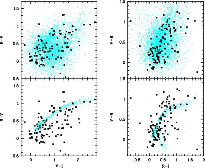
Figure 10: Optical colors for galaxies (top panels) and stars (bottom panels) in the field XMM-06. The black squares mark X-ray sources in this field with matches to the optical catalogs in all four passbands.

7 Summary

This paper describes the data products – reduced and stacked images as well as science-grade catalogs extracted from the latter – produced and released for the XMM-Newton follow-up survey performed with WFI at the ESO/MPG-2.2m telescope as part of the ESO Imaging Survey project. The survey was carried out as a collaboration between the EIS, XMM-Newton-SSC and IAEF-Bonn groups. At the time of writing 15 WFI fields (3.75 square degrees) have been observed for this survey of which 12 were released in the fall of 2004, with corrections to the weight maps in July 2005, and are described in this paper. For the 8 fields at high galactic latitude catalogs are also presented.

The images were reduced employing the EIS/MVM image processing library and photometrically calibrated using the EIS data reduction system. The EIS system was also used to produce more advanced survey products (stacks and catalogs), to assess their quality, and to make them publicly available via the web, together with comprehensive product logs. The quality of the data products reported in the logs is based on the comparison of different statistical measures such as galaxy and star number counts and the locus of stars in color-color diagrams with results obtained in previous works as well as predictions of theoretical models calibrated by independent studies. These diagnostics are regularly produced by the system forming an integral part of it.

In the particular case of this survey, a number of frames have been reduced by both EIS and the Bonn group, using independent software thus allowing a direct comparison of the resulting images and catalogs to be made. From this comparison one finds that the position of the sources extracted from images produced for the same field/filter combination by the different pipelines are in excellent agreement with a mean offset of $\sim$ 20 mas and a standard deviation of $\sim$ 50 mas. Comparison of the magnitudes of the extracted sources shows that in general the mean offset is $\lesssim 0.05$ mag, consistent with the estimated error of the photometric calibration of about $0.08$ mag. Cases with larger deviations were investigated further and the problem with the two most extreme cases were found to be unrelated to the calibration procedure. Instead, it demonstrates the need for the implementation of additional procedures to cope with the specific situation encountered and the need for a better calibration plan. This discussion illustrates a couple of important points. First, that while an automatic process is prone to errors in dealing with extreme but rare situations, reductions carried out with human intervention are prone to random errors which can never be eliminated. Second, more robust procedures can always be added or existing ones tuned to deal with exceptions once they are found. However, as always when dealing with automatic reduction of large volumes of data, the real issue is to decide on the trade-off between coping with these rare exceptions and the speed of the process and margin of failures one is willing to accept.

Finally, a comparison of the PSF distortions suggests that some improvement could be achieved by requiring the EIS/MVM to impose an additional constraint on the astrometric solution to improve the internal registration. As mentioned earlier this can be achieved by imposing the geometrical constraint that the CCDs form a mosaic.

Preliminary catalogs were also extracted from the available X-ray images and cross-correlated with the source lists produced from the $R$-band images. From this analysis one finds that about 61% of the X-ray sources have an optical counterpart within 2″, most of which are unique. Out of these about 70% are detected in all the available passbands. Combined, these results indicate that the adopted observing strategy successfully yields the expected results of producing a large population of X-ray sources ($\sim$ 300) with photometric information in four passbands, therefore enabling a tentative classification and redshift estimation, sufficiently faint to require follow-up observations with the VLT.

The present paper is one in the series presenting the results of a variety of optical/infrared surveys carried out by the EIS project.

Appendix A Comments on the individual fields

Below a broad overview of the 12 fields discussed in the present paper is given. It includes a description of their nature and the original target of the X-ray observations. Details about the exposure time per camera per observation are given on the web-page.

1. XMM-01/RX J0925.7$-$4758 – The original target was the ROSAT-discovered, galactic supersoft X-ray binary RX~J0925.7$-$4758, also known as MR~Vel (Motch et al. 1994). The X-ray image is a superposition of two medium deep ($\sim 60$ ks) observations with EPIC-PN in large window, EPIC-MOS1 in full frame, and EPIC-MOS2 in small window mode. This results in a reasonably deep ($\sim 115$ ks) exposure in the common PN and MOS area (less than half of the field of view).

2. XMM-02/RX J0720.4$-$3125 – Targeting the ROSAT-discovered isolated neutron star RX~J0720.4$-$3125 (Haberl et al. 1997), the X-ray image is a superposition of three medium deep observations with all cameras in full frame. The bright target of the observation causes visible out-of-time events (OOT) in the X-ray images leading to bright stripes through the target. These stripes are fixed in detector coordinates, hence they do not coincide in sky coordinates resulting in three different OOT stripes.

3. XMM-03/HE 1104$-$1805 – The primary target of this XMM-Newton observation was the double-lensed quasar HE~1104$-$1805 (Wisotzki et al. 1993). This is an empty field at high galactic latitude. The X-ray image is a combined image of the three EPIC cameras during the single observation of the target. Bad space weather resulted in a loss of $\sim$65% of the total exposure and a rather shallow resulting image ($\sim$10 ks).

4. XMM-04/MS1054.4$-$0321 – The galaxy cluster MS~1054.4$-$0321 at redshift of $z=0.83$ is the most distant cluster in the Einstein Medium Sensitive Survey and among the most massive ones (Gioia et al. 1990; Stocke et al. 1991; Gioia & Luppino 1994). The X-ray image is a combined image of the three EPIC cameras of the single observation of the target, all taken in full frame mode.

5. XMM-05/BPM 16274 – The white dwarf BPM~16274 is at high galactic latitude. This field is used for calibrations of the optical monitor on-board the XMM-Newton satellite. The X-ray image is a superposition of six observations in full frame mode of all three cameras. The archive contains already many more data sets with other camera settings and the observations in this field are ongoing.

6. XMM-06/RX J0505.3$-$2849 – This is a field at high galactic latitude. The galaxy cluster RX~J0505.3$-$2849 in the center was detected as part of the SHARC survey (Burke et al. 2003) at a redshift of $z=0.509$. The X-ray image is the superposition of all three EPIC cameras, which were all operated in full frame mode. Only the PN suffered significantly from high background, resulting in a medium deep X-ray image ($\sim$45 ks).

7. XMM-07/LBQS 2212$-$1759 – In order to avoid potential damage from the Leonid meteors when XMM intersects their trajectories annually, the spacecraft is oriented in the anti-Leonid direction for safety reasons. The field then repeatedly chosen for observation was centered on the $z=2.217$ quasar LBQS~2212$-$1759 (Barkhouse & Hall 2001). The X-ray image is a superposition of five observations with all cameras in full frame mode. Enhanced background affected less than 15% of the observations resulting in a truly deep field with more than 200 ks net exposure in all three cameras. The nominal target of the observations was not discovered, the image is thus dominated by the serendipitous source content. The most prominent source is a new cluster of galaxies close to the center of the field.

8. XMM-08/NGC 4666 – The target of this field was the almost edge-on spiral galaxy NGC~4666 which dominates the center of the field. Although the target was optically and X-ray extended, the target was included in the public survey since the target blocks only about 5% of the field of view. The X-ray image is a combined image of the three EPIC cameras of the single observation of the target, all taken in full frame mode.

9. XMM-09/QSO B1246$-$057 – The target was the broad absorption line quasar B1246$-$057. The XMM-Newton observation of the target was published by Grupe et al. (2003). The X-ray image is a combined image of the three EPIC cameras of the single observation of the target, all taken in full frame mode. The field is unusual, about one quarter of the field in the NE corner is almost devoid of X-ray sources. The dominant point-like object is the X-ray counterpart of the Algol binary HD~111487 (RBS~1165).

10. XMM-10/PB 5062 – PB~5062 (also known as QSO~B2202$-$0209) is a quasar at redshift $z=1.77$ (Yuan et al. 1998). The X-ray image is a combined image of the three EPIC cameras of the single observation of the target, all taken in full frame mode.

11. XMM-11/Sgr A – The target of this field is the center of our Milky Way. The X-ray image is a superposition of five observations with all cameras in full frame mode. The observations were severely affected by background flares resulting in a loss of more than 50% of the observation time. Nevertheless, repeated observations of the field resulted in a medium deep exposure with more than 40 ks exposure in all three cameras. The image is dominated by diffuse emission from the galactic center region. In addition there are two classes of point-sources, heavily absorbed, i.e. likely background sources with hard X-ray spectra and foreground sources with soft X-ray spectra.

12. XMM-12/WR 46 – This object also known as HD~104994 is a Wolf-Rayet star. The X-ray image is a combined image of the three EPIC cameras of the single observation of the target, all taken in full frame mode. Data loss due to enhanced background is insignificant resulting in a medium deep field with more than 70 ks exposure in each camera.

Appendix B Photometry

The photometric calibration is done in a fully automated way by the EIS Data Reduction System (da Costa et al., in preparation) calibrating all data to the Vega magnitude system. The photometric pipeline extracts catalogs from the standard star fields, and measures fluxes at different apertures to allow for a growth curve inspection. The positions and flux measurements for each object are cross-correlated with those corresponding to known standard stars as stored in a database. The matched standard stars are then used to determine the photometric zeropoint, extinction and color term from a linear fit. Finally, the zeropoint for each science frame is derived from the linear fit derived for the night of observation.

In the case of optical observations, as in this paper, the calibrations have been based on observations of Landolt (1992) standard star fields. The magnitudes were measured in 6″apertures, which from monitoring the growth curve of all measured stars proved to be adequate. The linear fits had from one to three free parameters depending on the available airmass and color coverage provided by the calibration plan. In cases where the airmass and/or color coverage is insufficient, pre-specified values for the extinction and color term, either determined from other solutions or from theoretical models, are used.

The photometric pipeline computes photometric parameters for all possible types of fits (one to three free parameters) and chooses the solution with the smallest rms to be the best solution for the night. A night is considered photometric if this scatter is less than a pre-defined value, which at the present time is taken to be 0.1 mag. If none of the solutions satisfies this criterion and/or the solution found yields unrealistic results (e.g. negative extinction) then the night is considered non-photometric and a default value for the zeropoint is adopted and its error set to $-1$. For nights without observation of standard star fields, a default zeropoint and an error of $-2$ are assigned to the image. Finally, during quality assessment of the data, calibrated images with zeropoints that deviate significantly from a reference value have the zeropoint in the header changed to a default value and its error set to $-3$. When a default value is assigned all images will have the same zeropoint in the header regardless of the airmass at which they were observed. For homogeneity, the default value normally adopted is the median of the zeropoints reported in the trend analysis kept by either the telescope team (depending on the instrument) or the internal EIS database. In the case of WFI, only one solution is currently reported on the WFI WWW pages.

The derived photometric solutions were used to calibrate the reduced images. The zeropoint in the header of a reduced image is given by

$$ZP=ZP^{\prime}-kX$$ (1)

where $ZP^{\prime}$ is the zeropoint at zero airmass (determined from the linear fit as described above), $k$ is the extinction coefficient and $X$ is the airmass at which the frame was observed. Using this definition the Vega magnitude can computed by

$$m_{\mathrm{Vega}}=-2.5\log(f)+ZP$$ (2)

where $f$ is the flux in number of counts directly measurable on the image (note that the reduced images are normalized to 1 s).

Appendix C Image stacks

Most fields are covered by more than one reduced image. These are co-added to create the final image product. The following steps are involved in the creation of a final stacked image:

• Grouping: reduced images are grouped into stacking blocks (SBs) according to position (with a minimum distance between centers of 0.25 times the field-of-view), and filter.

• Validation: as the co-addition is carried out in pixel space it is required that all images have been warped to the same reference grid. Therefore, images in a SB must share the same reference grid (projection, reference position, pixel scale and orientation). In addition, the images contributing to an SB, or their original RBs, are checked to ensure that they appear only once in the SB. Images in the SB are also checked to ensure that their flux scale has been properly normalized to 1 s, and if not they are re-normalized accordingly.

• Constraints: images in an SB are checked to ensure that they meet certain constraints, for instance on the value of seeing, the rms of the PSF distortion and grade. In addition, the contributing images to an SB, or their original RBs, are checked to prevent the repetition of raw exposures. Images not satisfying the constraints are discarded from the SB.

• PSF homogenization: all images in the SB are convolved by a Gaussian with a FWHM corresponding to the the largest value computed for the contributing images.

• Flux scale determination: before the images can be co-added, which is done using a weighted mean procedure, it is necessary to have all images at the same flux level. This is done by scaling photometric frames to zero airmass using the extinction coefficients from the photometric solutions. The non-photometric frames are scaled to the zero airmass level of the photometric frames (see below)

• Co-addition: images in a validated SB are co-added using a weighted mean. The weight images reflect the exposure times of their associated science image. Therefore, the weight of each image is a combination of exposure time and noise. However, the weight images also contain information about the location of bad pixels and masks which are set to zero weight and thus do not contribute to the final image. In the co-addition process, performed by the routine add-mosaic of the EIS/MVM library, a sigma-clipping procedure is employed to remove cosmic ray hits.

The image co-addition uses a weighted mean combination. The weighting is done with the weight images produced by the image reduction. Additionally, a thresholding procedure is employed to remove cosmic rays. In general, the use of weight maps and cosmic ray hits removal produces very clean final images.

As mentioned above, all images in an SB have to be scaled to a common flux level before the co-addition to assure the photometric calibration of the final, stacked image. For this rescaling, one has to consider two cases:

1. SB with at least one photometric frame – In this case the reference flux level is obtained from the combination of all contributing photometric frames. First, all photometrically calibrated frames are scaled to the flux level that would have been obtained at zero airmass. This is done using the extinction coefficients of their respective photometric solutions. Second, by computing a weighted average of all scaled images a reference image is created. For the final co-addition all input images (photometric and non-photometric) are scaled to the flux level of the reference image. The scaling factors are determined by comparing object magnitudes. Naturally, in cases where only one photometric frame is available, this one is used as the reference.

2. SB with no photometric frames – Occasionally, none of the reduced images in an SB are photometrically calibrated (e.g. no standards were observed in the night, observations in non-photometric nights). In such cases, all images are scaled to the flux level of an arbitrarily chosen reference image from the SB. The zeropoint of the final stacked image is then the zeropoint of the adopted reference image. The zeropoint of the output image is that of the arbitrarily chosen reference. These frames can be identified by the negative zeropoint error assigned to these cases, as described above.

Appendix D Catalog production

The final processing step in the EIS Data Reduction system is the creation of source catalogs by standardized procedures, resulting in catalogs containing enough information to be directly usable for scientific applications. Here the production of catalogs for deep, sparse fields is discussed. The production of catalogs for crowded fields, which are not included in this release, will be described in Zaggia et al. (2005, in preparation).

The EIS catalog production is based on SExtractor (Bertin & Arnouts 1996) and a common configuration file for all catalogs with a minimum number of adjustments to be made for individual images. For each image the appropriate values for the seeing and magnitude zeropoints as well as the weight-map associated to each image are used. Other parameters are the same for all catalogs.

The catalog production starts with a very low $S/N$ catalog, which contains a large number of spurious objects. To produce a science-grade catalog a number of steps are taken. First, the catalog is pruned for objects with a $S/N$ (determined from the MAGERR_AUTO) below a user-defined level, which was set to 5 for this release. The object magnitudes are converted to the AB system according to the response function of the optical system and corrected for galactic extinction. At present, this correction is applied to the magnitudes of all objects, including stars. To facilitate the use of the catalogs 14 flags are added for each object as described below.

The saturation level of the final image stack is difficult to determine from the input images due to variations in integration time and possibly seeing. Therefore, the saturation level is determined from the extracted catalog. The method is based on the FWHM and peak flux of bright objects. The distribution of the FWHM is determined and sigma-clipped to exclude bright galaxies from the sample. Among the remaining objects those with FWHM deviating more than $3\sigma$ are taken to be the saturated objects. The saturation level is set to the minimum peak value among these objects. This value is used to set the saturation flag.

To be able to remove objects close to bright stars masks can be created in two ways: by an automatic routine or by hand using a Skycat plug-in. The automatic masking adds masks around saturated objects as well as around objects brighter than a user-specified magnitude. The size of the mask scales with the major-axis of the object, as computed by SExtractor. The scaling factor is specified by the user. The adopted shape of the masks is a square with one of the diagonals oriented North-South in an attempt to mask the diffraction spikes. The parameters used in the mask definition are reported in the product log. The positions of all masks are reported in the MASKS table in the catalog.

Note that except for objects with $S/N$ less than that required, no object is removed from the catalog. If necessary, more objects can be pruned by the user according to the flags described below. In addition, the default magnitude system adopted for the objects can be changed using the information available in the FIELDS table.

The catalogs produced by the EIS Data Reduction system are in FITS format, based on the “Leiden Data Center” (LDAC) convention originally adopted by the DENIS project and later expanded in the course of the EIS project. It currently consists of a FITS header and the following tables: FIELDS, OBJECTS, MASK, and FILTER.

The FIELDS table contains general information for all objects in the catalogs. It consists of 109 columns including: (1) basic information set by the LDAC library; (2) keywords taken from the FITS header of the image from which the catalog was extracted; (3) the main SExtractor configuration parameters used; and (4) information computed by the EIS Data Reduction system. The latter includes, for instance:

• the diameter of the 10 apertures used for aperture magnitudes, ranging from 1″ to 5″ in steps of $0\aas@@fstack{\prime\prime}5$ and a large aperture of 10″;

• the WCS coordinates of the corners of the original image and of the trimmed area;

• the extinction correction. This is computed as the average of the value of the extinction in cells of $3\arcmin\times 3\arcmin$, distributed over the trimmed image;

• the value added to the original magnitude of the extracted objects in the Vega system to produce the reported magnitudes in the catalog in the AB system;

• an estimate of the fudge factor used to multiply the errors reported by SExtractor to correct for the correlated noise introduced by the re-sampling kernel;

• total and trimmed areas.

Some of the information contained in the FIELDS table is also available in the Product Logs which are available on the EIS XMM-Newton follow-up survey release pages.

The OBJECTS table reports the parameters characterizing the individual extracted objects as computed by SExtractor. It has 69 columns, some being vectors (e.g. aperture magnitudes), describing the main geometric and photometric properties of the objects. The parameters were chosen as a compromise between the total number of parameters and the most frequently requested parameters from survey product users. The choice of apertures and the flags defined are the result of suggestions made by users of EIS data products. In addition to the SExtractor flag, which are described in the SExtractor manual, 14 other flags have been defined to facilitate the filtering of the catalogs. These are

• FLAG_SEX1–FLAG_SEX128 – 8 flags individually representing the various SExtractor flag components;

• FLAG_SAT – set to 1 if the object is saturated;

• FLAG_TRIM – set to 1 if the object is inside a trimmed area;

• FLAG_MASK – set to 1 if the object is inside a masked area;

• EISFLAG – sum of FLAG_TRIM and FLAG_MASK

• FLAG_STATE – 1 if any of the above flags are set

• FLAG_STAR – 1 if star, 0 if galaxy, based on SExtractor’s CLASS_STAR parameter. The value used for separation and the magnitude down to which a classification was attempted are reported in the product log.

The MASK table gives the number and coordinates of the vertices of both automatically created masks as well as those drawn by hand using a Skycat plug-in.

The FILTER table gives the filter transmission curve and their convolution with the optical system response function.