Low Mass Pre-Main Sequence stars in the Large Magellanic Cloud - II: HST-WFPC2 observations of two fields in the 30 Doradus region

As a part of an ongoing effort to characterise the young stellar populations in the Large Magellanic Cloud, we present HST-WFPC2 broad and narrow band imaging of two fields with recent star formation activity in the Tarantula region. A population of objects with $\mathrm{H}\alpha$ and/or Balmer continuum excess was identified. On account of the intense $\mathrm{H}\alpha$ emission (equivalent widths up to several tens of Å), its correlation with the Balmer continuum excess and the stars’ location on the HR diagram, we interpret them as low mass ($\sim 1-2\leavevmode\nobreak\ M_{\sun}$) Pre-Main Sequence stars. In this framework, the data show that coeval high and low mass stars have significantly different spatial distributions, implying that star formation processes for different ranges of stellar masses are rather different and/or require different initial conditions. We find that the overall slope of the mass function of the young population is somewhat steeper than the classical Salpeter value and that the star formation density of this young component is $0.2-0.4\leavevmode\nobreak\ M_{\sun}\mathrm{yr}^{-1}\mathrm{kpc}^{-2}$, i.e. intermediate between the value for an active spiral disk and that of a starburst region. The uncertainties associated with the determination of the slope of the mass function and the star formation density are thoroughly discussed.

1 Introduction

Star-forming processes determine much of the appearance of the visible Universe: the shape of the Initial Mass Function (IMF) and its normalisation (the star-formation rate) are, together with stellar evolution theory, key ingredients in determining the chemical evolution of a galaxy and its stellar content. Yet, our theoretical understanding of the processes that lead from diffuse molecular clouds to stars is still very tentative, as many complex physical phenomena are simultaneously at play in producing the final results.

From an observational standpoint, most of the effort was traditionally devoted to nearby Galactic star-forming regions. If, on the one hand, studying them leads to the the best possible angular resolution, on the other hand, this is achieved at the expense of probing only a very limited set of astrophysical conditions (all these clouds have essentially solar metallicity, e.g. Padget padg96 (1996)). Also, they typically cover large areas on the sky that require extensive tiling to be fully covered with the current detectors (the Taurus star forming region, for example, covers as much as 12 degrees on the sky).

However, studying the effects of lower metallicity on star formation is essential to understand the evolution of both our own Galaxy, in which a large fraction of stars were formed at metallicities below solar, and of what is observed at high redshifts. As a matter of fact, the global star formation rate appears to have been much more vigorous (a factor of 10 or so) at $z\simeq 1.5$ than it is today (Madau et al mad96 (1996) and subsequent incarnations of the so-called “Madau plot”). At this epoch the mean metallicity of the interstellar gas was similar to that of the Large Magellanic Cloud (LMC, e.g. Pei, Fall & Hauser pei99 (1999)). This fact combined with the galaxy’s well-determined distance and small extinction makes the study of star forming regions in the LMC an important step towards understanding the general picture of galaxy evolution.

With a distance modulus of $18.57\pm 0.05$ (see the discussion in Romaniello et al rom00 (2000)), the LMC is the closest galactic companion to the Milky Way after the Sagittarius dwarf galaxy. At this distance one arcminute corresponds to roughly 15 pc and, thus, one pointing with most of the current generation of instruments comfortably covers almost any individual star forming region in the LMC (see, e.g., Hodge hod88 (1988)). In particular, the field of view of $2.5\arcmin\times 2.5\arcmin$ of the camera we have used, the WFPC2 on board the HST, corresponds to $37\times 37\leavevmode\nobreak\ \mathrm{pc}^{2}$ and leads to the detection of several thousands of stars per pointing. The LMC is especially suited for stellar populations studies for two additional reasons. First, its depth along the line of sight is negligible, at least in the central parts we consider (van der Marel & Cioni mar01 (2001)), and all the stars can be effectively considered at the same distance, thus minimising a spurious scatter in the Colour-Magnitude Diagrams (CMDs). Second, the extinction in its direction due to dust in our Galaxy is low, about $\mathrm{E}(\mathrm{B}-\mathrm{V})\simeq 0.05$ (Bessell bes91 (1991), Schwering sch91 (1991)), and hence, our view is not severely obstructed.

The advent of the Hubble Space Telescope (HST) has for the first time made it possible to observationally tackle the open questions about star formation in outer galaxies and, in particular, in the LMC, down to a solar mass or even lower. Some of the evidence from ground and HST-based studies shows that there may be significant differences between star formation processes in the LMC and in the Galaxy. Immediately after the first HST refurbishment mission, the observations of the double cluster NGC 1850 in the LMC made with Wide Field Camera 2 (WFPC2) have provided the first detection of a population of Pre-Main-Sequence (PMS) stars (Gilmozzi et al 1994) in an extragalactic star forming region. The evidence was purely statistical, in the sense that the existence of PMS stars was deduced by the presence of many stars that were lying above the main sequence and whose number (almost 400) could not be accounted for by any evolved population. Subsequently, Romaniello (1998), Panagia et al. (2000) and Romaniello et al (2002), by comparison of the magnitudes obtained with an $H\alpha$ narrow band filter (F656N) with those taken with a broad band red filter(F675W), measured the equivalent width of the $H\alpha$ emission for several hundred of candidates PMS stars in the field around SN 1987A, thus confirming their PMS identification unambiguously. Eventually, the first spectroscopically confirmed discovery of a bona-fide T Tauri star in the LMC, LTS J054427-692659, a low-mass, late-type star located within the dark cloud Hodge II 139, was reported by Wichmann, Schmitt & Krautter (wic01 (2001)).

Some of the evidence from ground and HST-based studies shows that there may be significant differences between star formation processes in the LMC and in the Galaxy. For example, Lamers et al (lam99 (1999)) and de Wit et al (wit02 (2002)), on the basis of ground-based data, have suggested the presence of high-mass Pre-Main Sequence stars in the LMC (Herbig AeBe stars, but see the caveats in de Wit et al wit05 (2005)) with luminosities systematically higher than observed in our Galaxy, and located well above the “birthline” of Palla & Stahler (ps91 (1991)). They attribute this finding either to a shorter accretion timescale in the LMC or to its smaller dust-to-gas ratio. Whether such differences in the physical conditions under which stars form will generally lead to differences at the low mass end is an open question, but Panagia et al (pan00 (2000), Paper I) and Romaniello et al (rom04 (2004)) offer tantalising evidence in this direction.

HST-based studies of the IMF in the LMC (which have mostly concentrated on young, compact clusters) have in fact produced, for the lower masses, often discrepant results. On the one hand, there is widespread agreement that the IMF for $M>3M_{\sun}$ is similar to the mean Galactic one (i.e. a “Salpeter function”, a power-law with slope $\alpha=-2.35$). On the other hand, though, the results for the lower masses ($1M_{\sun}\lesssim M\lesssim 3M_{\sun}$) are rather difficult to reconcile with each other, with different authors finding (in different regions, or even in the same one) very different slopes, ranging from very steep IMFs ($\alpha\simeq-3$, Mateo mat88 (1988)) to quite shallow ones ($\alpha\simeq-1$, Sirianni et al sir00 (2000)) with many intermediate values represented.

As a part of an ongoing effort to characterise the young stellar population in the LMC, we have applied the techniques developed by Romaniello (rom98 (1998)) to detect and characterise low mass Pre-Main Sequence (PMS) stars in two regions of recent star formation observed with the WFPC2 on board the HST. The fields were selected in the HST archive so as to have deep narrow-band $\mathrm{H}\alpha$ observations, which, as we shall see, are fundamental to detect the low mass Pre-Main Sequence populations. Both fields are in the proximity of Supernova~1987A (SN1987A), whose immediate vicinities we have already studied with similar methods (Romaniello rom98 (1998), Panagia et al pan00 (2000), Romaniello et al rom04 (2004)). In addition to $\mathrm{H}\alpha$, one of the two fields presented here was imaged in four broad band filters, so that this wealth of data allowed us to recover the intrinsic properties of the stars as well as their reddening following the prescriptions developed by Romaniello et al (rom02 (2002)). For the other field the broad band data were limited to two filters only, and, therefore, the analysis had to be necessarily cruder. We will, however, show how interesting conclusions on the properties of the stellar populations can be drawn also from such a limited dataset. More fields are in the process of being analysed to enlarge our study of young populations in the Magellanic Clouds across the mass spectrum.

Section 2 is devoted to the description of the datasets and the reduction techniques, whereas the results for the two fields considered here are discussed in section 3 and 4. Finally, summary and conclusions are presented in section 5.

2 Observations and data reduction

We have taken advantage of the vast HST archive to select two LMC fields with recent star formation activity. They were chosen for having both broad-band and $\mathrm{H}\alpha$ observations, which, as we shall see in section 3.4, is a fundamental requirement to identify the low mass Pre-Main Sequence stars, and unambiguously disentangle them from the much older field subgiants.

The two fields we present in this paper are located some $20\arcmin$ southwest of the 30~Doradus nebula. This area includes regions of very active star formation, in which different groups of early type stars are interspersed with HII regions and Supernova remnant shells, as well as one of the best know objects in the entire sky: Supernova 1987A. The footprints of the WFPC2 pointings superimposed on a DSS image are shown in Figure 1. Also shown in the same Figure are the locations of the fields around SN1987A itself in which Panagia et al (pan00 (2000)) and and Romaniello et al (rom04 (2004)) have identified nearly 500 Pre-Main Sequence candidates through their $\mathrm{H}\alpha$ and Balmer continuum emission.

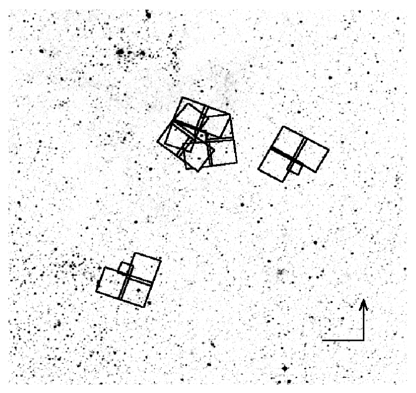
Figure 1: Footprints of the WFPC2 pointings superposed to a DSS image $20\arcmin$ on the side. The progenitor of SN1987A is visible at the centre of the three WFPC2 fields of Panagia et al (pan00 (2000)). The 30 Doradus nebula is roughly $20\arcmin$ to the northeast.

The centres of the fields are located at $\alpha=05:36:11.57$, $\delta=-69:23:00.74$ (J2000) and $\alpha=05:34:38.01$, $\delta=-69:17:14.90$ (J2000). Given their position with respect to the SN1987A, in the following we will refer to the pointings described here as South field and West field, respectively. Their angular separations from SN1987A are $8\arcmin$ and $4.5\arcmin$ (i.e. 120 and 68 pc in projection), respectively, and the South field is just $2.5\arcmin$ west of the young cluster NGC~2050. The logs of the observations of the two fields are reported in Table 1 and 2. The detailed description of the WFPC2 camera and its filters can be found in the corresponding Instrument Handbook (Heyer et al wfpc2 (2004)).

Filter Name	Exposure Time (s)	Comments
F300W	$600+1200$	Wide U
F450W	$50+200$	Wide B
F675W	$50+200$	R-like
F814W	$140+400$	I-like
F656N	$1200+1200+1300$	$\mathrm{H}\alpha$

Table 1: Log of the observations of the South field. They were taken on January, $1^{\mathrm{st}}$ 1997, under proposal number 6437, PI Robert P. Kirshner.

Filter Name	Exposure Time (s)	Comments
F547M	$2\times 120^{\mathrm{a}}$	V-like
F675W	$2\times 120^{\mathrm{a}}$	R-like
F656N	$1000+2\times 2000^{\mathrm{a}}$	$\mathrm{H}\alpha$
	$900+1000+2000^{\mathrm{b}}$

Table 2: Log of the observations of the West field. The proposal number is 6033, PI Jeremy Walsh.

The data were processed through the standard Post Observation Data Processing System pipeline for bias removal and flat fielding. In all cases the cosmic ray events were removed combining the available images, duly registered.

The plate scale of the camera is 0.045 and 0.099 arcsec/pixel in the PC and in the three WF chips, respectively. We performed aperture photometry following the prescriptions by Gilmozzi (gil90 (1990)) as refined by Romaniello (rom98 (1998)), i.e. measuring the flux in a circular aperture of 2 pixels radius and the sky background value in an annulus of internal radius 3 pixels and width 2 pixels. Due to the undersampling of the WFPC2 PSF, this prescription leads to a smaller dispersion in the Colour-Magnitude Diagrams, i.e. better photometry, than PSF fitting for non-jittered observations of marginally crowded fields (Cool & King coo95 (1995), Romaniello rom98 (1998)). The photometric error is computed taking into account the poissonian statistics of the flux from the source and the measured rms of the flux from the sky background around it. This latter includes the effects of poissonian fluctuations on the background emission, flat-fielding errors, etc.

Photometry for the saturated stars was recovered by either fitting the unsaturated wings of the PSF for stars with no saturation outside the central 2 pixel radius, or by following the method developed by Gilliland (gil94 (1994)) for the heavily saturated ones.

The flux calibration was obtained using the internal calibration of the WFPC2 (Whitmore whit95 (1995)), which is typically accurate to within 5% at optical wavelengths. The spectrum of Vega is used to set the photometric zeropoints (VEGAMAG system).

3 The South field

The F450W (B), F675W (R) and F656N ($\mathrm{H}\alpha$) composite image of the South field is shown in Figure 2.

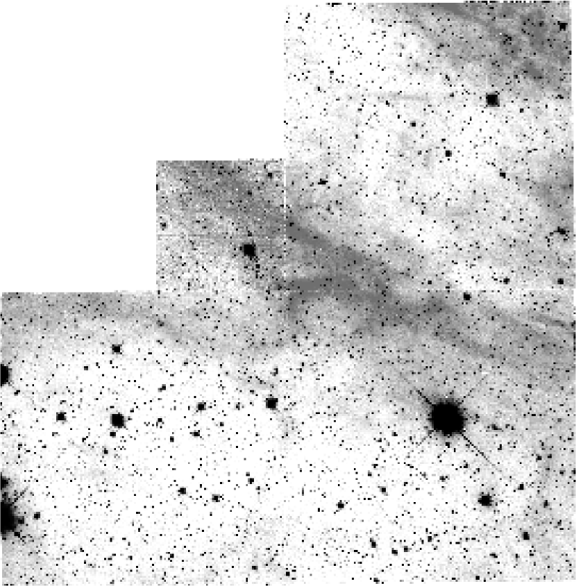
Figure 2: The South field as observed in the combination of F450W (B), F675W (R) and F656N ($\mathrm{H}\alpha$) filters.

We have detected 13,098 stars in the whole field, 4,108 of which with a mean error in the 4 broad bands lower than 0.1 mag:

$$\bar{\delta}_{4}=\sqrt{\frac{\delta{{}_{\mathrm{F300W}}^{2}}+\delta{{}_{\mathrm{F450W}}^{2}}+\delta{{}_{\mathrm{F675W}}^{2}}+\delta{{}_{\mathrm{F814W}}^{2}}}{4}}<0.1$$ (1)

The brightest star in the field, located in the WF3 chip, is so badly saturated that it was impossible to measure its magnitude from the WFPC2 images. On the other hand, it is a well known star, Sk~-69~211 (Sanduleak sand69 (1969)), also known as HDE~269832, and its accurate photometry is available from ground-based studies. Fitzpatrick (fit88 (1988)) classifies it as B9Ia supergiant with V$=10.36$, B$-$V$=0.09$ and $\mathrm{E}(\mathrm{B}-\mathrm{V})\simeq 0.1$. With a radial velocity of $+272\leavevmode\nobreak\ \mathrm{km\leavevmode\nobreak\ s}^{-1}$ it is a bona fide member of the LMC (Ardeberg et al ard72 (1972)). Using the temperature scale and bolometric corrections of Schmidt-Kaler (sk82 (1982)), one derives for it an effective temperature of roughly 10,000 K and a luminosity of roughly $3\cdot 10^{5}$ L_☉.

The Colour-Magnitude Diagrams for four combination of filters are shown in Figure 3.

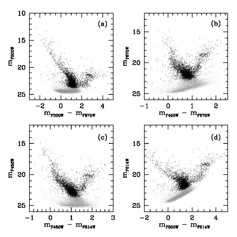
Figure 3: Colour-Magnitude diagrams of the 13,098 stars detected in the South field for four combination of filters. The black dots are the 4,108 stars with a mean photometric error in the four bands ($\bar{\delta}_{4}$, see equation 1) smaller than 0.1 mag. Sk -69 211 is not shown.

The presence of at least two distinct populations is readily detected in Figure 3. The first one is associated with the feature extending up to $m_{\mathrm{F450W}}\simeq\leavevmode\nobreak\ 15$ and with a colour $(m_{\mathrm{F450W}}-m_{\mathrm{F814W}})\simeq-0.6$ (see panel (c)). Of course, this is a young generation of stars still on or just off the Zero Age Main-Sequence. The old population of the LMC field, with ages in excess of 500 Myr or so, is identified by the presence of the Red Clump at $m_{\mathrm{F450W}}\simeq\leavevmode\nobreak\ 20$, $(m_{\mathrm{F450W}}-m_{\mathrm{F814W}})\simeq\leavevmode\nobreak\ 1.8$ and an extended Red Giant Branch reaching magnitudes as bright as $m_{\mathrm{F450W}}\simeq\leavevmode\nobreak\ 18$ at $(m_{\mathrm{F450W}}-m_{\mathrm{F814W}})\simeq\leavevmode\nobreak\ 3$.

3.1 Reddening distribution

In order to derive the detailed properties of the stars in the field we first have to determine the interstellar reddening. As in any region of recent star formation, one can expect the stars to be still entwined with the material they were formed from and, hence, the interstellar reddening to be spatially inhomogeneous. We have, then, applied the procedure developed by Romaniello et al (rom02 (2002)) to measure $\mathrm{E}(\mathrm{B}-\mathrm{V})$, $\mathrm{T}_{eff}$ and luminosities for individual stars. We have used a value for the distance to the LMC of 51.8 kpc (Romaniello et al rom00 (2000)). In brief, the procedure consists in a fit of the observed fluxes to a grid of theoretical ones, reddened by various amounts of $\mathrm{E}(\mathrm{B}-\mathrm{V})$. A minimum $\chi^{2}$ technique is, then, used to identify the best combination of $\mathrm{T}_{eff}$, $\mathrm{E}(\mathrm{B}-\mathrm{V})$ and luminosities, with their associated errors. As inputs for the fit we have used the atmosphere models by Bessell et al (bes98 (1998)) and the reddening law appropriate for this region of the LMC as derived by Scuderi et al (scud96 (1996)) from a study of Star~2, one of the two stars projected within a few arcseconds from SN1987A.

We were able to estimate $\mathrm{E}(\mathrm{B}-\mathrm{V})$ for 1,205 stars, i.e. 9% of the total or one every 4 square arcseconds on average, while for the others we have used the mean value of their neighbours with direct measurements (cf. Romaniello et al rom02 (2002)). An inspection of Figure 10, which will be discussed in detail in section 3.3.2, shows that the location of the dereddened stars in the $(m_{\mathrm{F300W,0}}-m_{\mathrm{F450W,0}})$ vs $(m_{\mathrm{F450W,0}}-m_{\mathrm{F814W,0}})$ colour-colour plane generally agrees very well with the expectations from the Bessell et al (bes98 (1998)) model atmospheres, with a scatter consistent with observational errors ($\bar{\delta}_{4}\lesssim 0.1$, the discrepancy observed for some stars at $(m_{\mathrm{F450W,0}}-m_{\mathrm{F814W,0}})\simeq 0.7$ is thoroughly discussed in section 3.3.2). This agreement, then, gives us confidence on the use of the Bessel et al (bes98 (1998)) atmospheres to reproduce the observed colors and confirms that our dereddening procedure does not introduce any significant systematic effect (see also Romaniello et al rom02 (2002)).

The derived reddening distribution is indeed rather clumpy, as shown in Figure 4. The mean extinction over the field is $\mathrm{E}(\mathrm{B}-\mathrm{V})=0.180$ (second column of Table 3), i.e. comparable to the mode of the distribution for the old population of the LMC as a whole of $\mathrm{E}(\mathrm{B}-\mathrm{V})\simeq 0.1$ (Zaritsky zar99 (1999)). The corresponding rms is 0.091 (third column). Thanks to the large number of stars, then, the error on the mean is negligible, i.e. $0.091/\sqrt{(}1205)=0.003$. Again from Table 3, one sees that the mean formal error on the individual reddening determination due to the combined effects of photometric errors and fitting uncertainties (fourth column) is 0.029 magnitudes. This, together with the measured rms, implies that the intrinsic dispersion in $\mathrm{E}(\mathrm{B}-\mathrm{V})$ due to the patchy distribution of dust is 0.086 magnitudes. This value is both statistically significant and non negligible, considering that it reflects itself in a spread of about $0.086\times 5.5\simeq 0.5$ mag in F300W, $0.086\times 3.9\simeq 0.3$ mag in F450W, $0.086\times 2.4\simeq 0.2$ mag F675W and $0.086\times 1.9\simeq 0.15$ mag in F814W (see Table 8 of Romaniello et al rom02 (2002) for the extinction coefficients in the WFPC2 bands).

Figure 4: Spatial distribution of stars with high ($\mathrm{E}(\mathrm{B}-\mathrm{V})>0.3$, filled circles) and low ($\mathrm{E}(\mathrm{B}-\mathrm{V})<0.1$, open circles) reddening. The average reddening is significantly higher in the WF2 chip, i.e. towards NGC 2050 (see Figure 1).

It is also clear from Figure 4 that the interstellar extinction is inhomogeneous on larger scales as well, with the reddening being significantly higher in the PC and WF2 chips, i.e. in the direction of NGC 2050, than elsewhere. The actual numbers are reported in Table 3, where one can see that the difference in the mean reddening between the PC and WF2 chips on the one side and the WF3 and WF4 chips on the other is statistically highly significant. The dispersion, on the other hand, is almost constant across the chips (see also section 3.5.1). All of these facts highlight once more how crucial it is to accurately deredden the stars in order to recover and interpret their properties.

Chip	Mean	rms	Error	Dispersion	No. of stars
PC	0.233	0.117	0.037	0.112	33
WF2	0.210	0.093	0.027	0.089	401
WF3	0.157	0.089	0.031	0.083	427
WF4	0.168	0.077	0.028	0.072	344
All	0.180	0.091	0.029	0.086	1,205

Table 3: Spatial distribution of $\mathrm{E}(\mathrm{B}-\mathrm{V})$ colour excess as measured in the South field. In column 3 we report the measured rms of the $\mathrm{E}(\mathrm{B}-\mathrm{V})$ distribution, in column 4 the mean error on $\mathrm{E}(\mathrm{B}-\mathrm{V})$ resulting from the fitting procedure (see text), whereas column 5 lists the intrinsic reddening dispersion, computed as the quadratic difference of the first two quantities. The number of stars with direct extinction determination is shown in the last column.

Finally, it is interesting to notice that the spatial distribution of $\mathrm{E}(\mathrm{B}-\mathrm{V})$ does not correlate with the diffuse $\mathrm{H}\alpha$ emission, which is highest across the PC and the upper part of the WF3 chips, whereas it is quite faint in the WF2 chip (see Figure 2).

3.2 HR diagram

Once dereddened, the stars can accurately be placed in the HR diagram and their properties derived by comparing their positions with theoretical models (Figure 5).

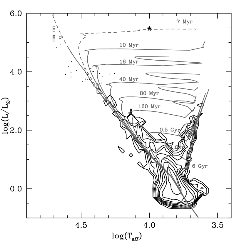
Figure 5: Hess diagram for the 13,098 stars in the South field. The open squares indicate 6 stars for which the F300W magnitude is ill determined because of saturation and, hence, the fit was performed excluding this filter. All of them, but one, require a temperature equal to or larger than 50,000 K, the highest available for the model atmospheres by Bessell et al (bes98 (1998)). The location of Sk -69 211 according to the photometry by Fitzpatrick (fit88 (1988)) is shown with a star symbol. The ZAMS and selected isochrones for Z$=0.3\cdot\mathrm{Z}_{\sun}$ by Brocato & Castellani (bc93 (1993)) and Cassisi et al (ccs94 (1993)) are overlaid to the data (grey solid lines). These models only extend to $25\leavevmode\nobreak\ M_{\sun}$, so we have complemented them with those of Schaerer et al (sch93 (1993)) for higher masses (grey dashed lines).

As we have already noticed from an inspection of the CMDs shown in Figure 3, no single age can explain the distribution of stars as observed in the HR diagram of the South field. Starting from the top-left corner of the HR diagram, the most massive stars, plotted as open squares in Figure 5, have masses of the order of $40\leavevmode\nobreak\ M_{\sun}$ and, thus, are definitely younger than 5 Myr. Since they are severely affected by saturation in both F300W exposures, their intrinsic parameters were derived excluding the flux in this filter from the fit. As discussed by Romaniello et al (rom02 (2002)), lacking the UV information, the fit is rather uncertain. In any case, all of them, but one, seem to require temperatures higher than 50,000 K, the highest available for the Bessell et al (bes98 (1998)) models. In conclusion, although their stellar parameters cannot be accurately measured, these stars are certainly massive and, hence, young, even more so than their position in the HR diagram would indicate.

With a comparable bolometric luminosity, but a much lower temperature, there is Sk -69 211. It falls exactly on the 7 Myr isochrone by Schaerer et al (sch93 (1993)), i.e. it is without a doubt older than the bluest stars in the field. A comparison with stellar evolutionary models assigns a mass of roughly $27\leavevmode\nobreak\ \mathrm{M}_{\sun}$ to it. Interestingly, a similar phenomenon was reported in Galactic OB associations by Massey et al (mas95 (1995)), who noted the “occasional presence of an evolved star” among a younger population.

Finally, stars with ages between a few tens of million and several billion years are required to account for the stars at lower luminosities.

3.3 A population of peculiar objects

A population of peculiar objects was detected in the South field by means of their $\mathrm{H}\alpha$ and Balmer continuum excesses (the two emissions positively correlate, as we shall see in section 3.3.2). In this section we describe the selection criteria for these stars and offer a possible explanation of their nature as Pre-Main Sequence stars.

3.3.1 $\mathrm{H}\alpha$ emission

Following Romaniello (rom98 (1998); see also Panagia et al pan00 (2000) and Romaniello et al rom04 (2004)), we compare the magnitudes in the R band (F675W) with the ones measured with the narrow band $\mathrm{H}\alpha$ filter (F656N) to identify stars with a sufficiently strong $\mathrm{H}\alpha$ emission. As it can be seen in Figure 2 there is significant nebular $\mathrm{H}\alpha$ emission in the South field. It is distributed in filaments with a typical length of several tens of arcseconds up to several arcminutes. All of the stars that are found to have $\mathrm{H}\alpha$ emission (see below) were inspected by eye to ensure that the nebular contribution was properly subtracted from the narrow band photometry.

In order to select stars with a statistically significant $\mathrm{H}\alpha$ emission we have compared the observed histogram of $(m_{\mathrm{F675W}}-m_{\mathrm{F656N}})$ for the stars in the field with the distribution expected if no emission was present. This latter was derived with the following four steps:

Figure 6: Relation between the WFPC2 $(m_{\mathrm{F675W}}-m_{\mathrm{F656N}})$ colour (i.e. $\mathrm{R}-\mathrm{H}\alpha$) and effective temperature as derived from Kurucz (kur93 (1993)) model atmospheres (see text).

1. Kurucz (kur93 (1993)) model atmospheres for a metallicity $[\mathrm{M}/\mathrm{H}]=-0.5$ at different effective temperatures were used to compute synthetic spectra between 5,700 and 7,800 Å, the region covered by the F675W filter. A spectral resolution of 1 Å was chosen, so as to sample the $\mathrm{H}\alpha$ line to a much better accuracy than the FWHM of the WFPC2 F656N filter ($\sim 20$ Å, Heyer et al wfpc2 (2004)).

2. These spectra were fed to the synphot task in IRAF to yield the expected $(m_{\mathrm{F675W}}-m_{\mathrm{F656N}})$ colour of “normal” stars, i.e. with $\mathrm{H}\alpha$ in absorption, as a function of their effective temperature. The resulting relation is shown in Figure 6.

3. We have used this relation together with the measure effective temperatures of the stars (cfr section 3.2) to compute the expected $(m_{\mathrm{F675W}}-m_{\mathrm{F656N}})$ colour for our stars in the absence of any $\mathrm{H}\alpha$ emission (shaded area in Figure 7).

4. Finally, this intrinsic distribution was broadened by the measured photometric error on the $(m_{\mathrm{F675W}}-m_{\mathrm{F656N}})$ colour. To this end, the intrinsic distribution was convolved with the appropriate error function, i.e. the normalised sum of the error Gaussians of the individual stars. This is, then, the colour distribution that the stars in the field are expected to have according to their measured temperature.

The comparison of the observed and expected distributions derived as described above is presented in Figure 7 (solid and dashed lines, respectively). The left-hand tails of the two distributions are in good agreement with each other, implying that the broadening towards negative values of $(m_{\mathrm{F675W}}-m_{\mathrm{F656N}})$ compared to the intrinsic, error-free distribution (shaded area in Figure 7) is caused by photometric errors. Moving towards more positive $(m_{\mathrm{F675W}}-m_{\mathrm{F656N}})$ values, however, the two histograms become increasingly discrepant, until an excess of observed stars with positive $(m_{\mathrm{F675W}}-m_{\mathrm{F656N}})$ colours, i.e. $\mathrm{H}\alpha$ emission, compared to the expectations is evident for $(m_{\mathrm{F675W}}-m_{\mathrm{F656N}})\gtrsim 0.2$ (dots in Figure 7). Applying a $\chi^{2}$ test confirms that the distribution are conclusively different ($\tilde{\chi}^{2}=11$).

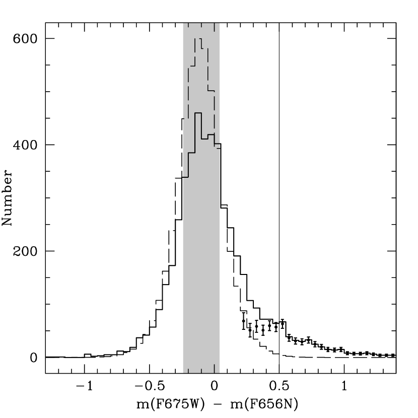
Figure 7: Observed (thick solid line) and expected (thin dashed line, see text) distribution of $(m_{\mathrm{F675W}}-m_{\mathrm{F656N}})$ colour in the South field. The histograms contain 4,938 stars, those with a positive detection in the F656N ($\mathrm{H}\alpha$). The shaded areas marks the intrinsic colour interval predicted by the atmosphere models, i.e. without the effect of observational errors (see also Figure 6). As it can be seen, the left-hand tails of the two histograms are in agreement, and the excess of observed stars with positive $(m_{\mathrm{F675W}}-m_{\mathrm{F656N}})$ colours, i.e. $\mathrm{H}\alpha$ emission, compared to the expectations is evident for $(m_{\mathrm{F675W}}-m_{\mathrm{F656N}})\gtrsim 0.2$. The distribution of the stars with significant excess (see text) is shown as dots, together with the corresponding errorbars. The value of the excess above which stars can be identified individually is marked with a vertical line.

In Figure 8 we report the observed and expected $(m_{\mathrm{F675W}}-m_{\mathrm{F656N}})$ distributions, derived as described above, broken down in different intervals of observational uncertainty $\delta(m_{\mathrm{F675W}}-m_{\mathrm{F656N}})$. The error range used is quoted in each panel. Since the photometric error is dominated by Poisson noise on photon statistics, the intervals in error are essentially intervals in $m_{\mathrm{F675W}}$ magnitude (reported within brackets in each panel). In all cases the widths of the left-hand side of the observed and expected distributions agree, confirming that the broadening is, indeed, due to photometric errors, whereas an excess of $\mathrm{H}\alpha$-emitting stars is detected at $(m_{\mathrm{F675W}}-m_{\mathrm{F656N}})\gtrsim 0.2$.

Figure 8: Same as Figure 7, but each panel only contains the stars in the quoted range of error on the $m_{\mathrm{F675W}}-m_{\mathrm{F656N}}$ colour. The corresponding approximate range in $m_{\mathrm{F675W}}$ magnitude is also reported in each panel. The value of the excess above which stars can be identified individually is marked with a vertical line in each panel.

Based on the distributions of Figure 7 and 8, we use the following criteria to identify the stars with a statistically significant excess:

• the stars that populate $(m_{\mathrm{F675W}}-m_{\mathrm{F656N}})$ bins in which the observed distribution exceeds the expected one by 3 Poissonian standard deviations or more;

• while the criterion above ensures a high statistical significance of the selected objects, by definition it excludes stars in scarcely populated bins, i.e. with less than 9 stars. To compensate for this, we also include in the sample the stars for which the $(m_{\mathrm{F675W}}-m_{\mathrm{F656N}})$ excess itself is highly significant, i.e. $(m_{\mathrm{F675W}}-m_{\mathrm{F656N}})>3\cdot\delta(m_{\mathrm{F675W}}-m_{\mathrm{F656N}})$, even if they belong to sparse bins. This only adds roughly 1% of the stars to the sample, but they are important ones because they have the highest $\mathrm{H}\alpha$ emission and, hence, are the most active ones.

In total, there are $781\pm 33$ stars that satisfy the criteria above. Their distribution, with the associated error bars, is shown in Figure 7 as dots. These errors are the statistical ones that pertain to this particular dataset. Deeper observations, most notably in the $\mathrm{H}\alpha$ F656N filter, would lead to a higher number of detections (see the discussion in section 4.2).

The number of excess stars in each panel of Figure 8 is reported in Table 4, together with the ratio of the total number of stars to that of the excess stars, from where one can see that roughly 40% of the 781 $\mathrm{H}\alpha$ emitters have quite good photometry, i.e. an error smaller than 0.2 mag. This generally implies errors in both bands less than 0.14, i.e. a 7 sigma detection.

Error range	Number of	Ratio
	excess stars	(total/excess)
$0.05-0.10$	$7\pm 3$	135
$0.10-0.15$	$74\pm 9$	16
$0.15-0.20$	$205\pm 15$	5
$0.20-0.25$	$264\pm 18$	4
$0.25-0.30$	$231\pm 15$	4

Table 4: Distribution of $\mathrm{H}\alpha$ excess stars in different bins of uncertainty on the $\mathrm{H}\alpha$ color index $m_{\mathrm{F675W}}-m_{\mathrm{F656N}}$ (see text and Figure 8).

It is clear from the discussion above that the objects with $\mathrm{H}\alpha$ excess can be divided in two groups, according the the strength of the $(m_{\mathrm{F675W}}-m_{\mathrm{F656N}})$ excess. If it is so strong that no “normal” star is expected to match it, i.e. if the dashed histogram in Figure 7 is 0, then the stars can be pinpointed one by one. As it can be seen in Figure 7 the condition that the expected histogram be 0 corresponds to $(m_{\mathrm{F675W}}-m_{\mathrm{F656N}})\gtrsim 0.5$ (or EW$(\mathrm{H}\alpha)\gtrsim 17$ Å, see appendix A). There are 366 such stars out of the total 781 with $\mathrm{H}\alpha$ excess (47%). If, on the other hand, the expected number of stars (dashed histogram in Figure 7) is not zero (i.e. $m_{\mathrm{F675W}}-m_{\mathrm{F656N}}\lesssim 0.5$), excess stars can only be identified statistically, but not on a one-to-one basis.

The distribution of the $\mathrm{H}\alpha$ equivalent widths (EW) for the 781 stars with statistically significant excess is displayed in Figure 9. The observed colour excesses $(m_{\mathrm{F675W}}-m_{\mathrm{F656N}})$ were converted into to equivalent widths using the relation derived in appendix A and plotted in Figure 19. The sharp drop at low values of the equivalent width is not real, but, rather, an artifact of our selection criteria that can only identify emission line objects above $(m_{\mathrm{F675W}}-m_{\mathrm{F656N}})\gtrsim 0.2$, i.e. $\mathrm{EW}(\mathrm{H}\alpha)\gtrsim 6$ Å, the weaker ones being lost in the noise.

Figure 9: Distribution of $\mathrm{H}\alpha$ equivalent widths for the 781 stars with statistically significant excess. The observed colour excesses $(m_{\mathrm{F675W}}-m_{\mathrm{F656N}})$ were converted to equivalent widths using the relation derived in appendix A and displayed in Figure 19. The dashed vertical line marks the excess above which we can identify the emission-line stars unambiguously ($m_{\mathrm{F675W}}-m_{\mathrm{F656N}}>0.5$, corresponding to EW$(\mathrm{H}\alpha)>17$ Å).

3.3.2 Balmer continuum excess

Objects in the South field exhibit yet another spectral peculiarity in addition to $\mathrm{H}\alpha$ emission: excess continuum emission blueward of the Balmer jump at 3646 Å, i.e. between the F300W and F450W WFPC2 filters.

The occurrence of this excess emission can be readily seen in Figure 10 where we plot the dereddened $(m_{\mathrm{F300W,0}}-m_{\mathrm{F450W,0}})$ vs $(m_{\mathrm{F450W,0}}-m_{\mathrm{F814W,0}})$ colours for stars with overall good photometry ($\bar{\delta}_{4}<0.1$, see equation 1). For reference, the expected locus from the stellar atmosphere models of Bessell et al (bes98 (1998)) for $Z=0.3\cdot Z_{\sun}$ and $\log(g)=4.5$ is shown as a solid line. As we have already noticed in section 3.1, there is a general very good agreement between the locus of the dereddened stars and the expectations from the models atmospheres, with a scatter consistent with observational errors. Thus, the asymmetric broadening compared to the models at $(m_{\mathrm{F450W,0}}-m_{\mathrm{F814W,0}})\simeq 0.7$ cannot be due to photometric errors (in fact, the broadening towards redder $(m_{\mathrm{F300W,0}}-m_{\mathrm{F450W,0}})$ colours is consistent with the errors, the one to the blue is not). Rather, it has to be ascribed to genuine deviations in the objects’ spectra relative to a bare photosphere, as represented by the solid line.

Figure 10: Dereddened $(m_{\mathrm{F300W,0}}-m_{\mathrm{F450W,0}})$ vs $(m_{\mathrm{F450W,0}}-m_{\mathrm{F814W,0}})$ colour-colour diagram for the stars in the South field with a mean error in the 4 wide bands ($\bar{\delta}_{4}$, see equation 1) smaller than 0.1. The theoretical locus from the stellar atmosphere models of Bessell et al (bes98 (1998)) is shown as a solid line and the expected $(m_{\mathrm{F300W,0}}-m_{\mathrm{F450W,0}})$ colour at $(m_{\mathrm{F450W,0}}-m_{\mathrm{F814W,0}})=0.7$ is marked by the thin vertical line. The horizontal dashed lines highlight the region used to select stars in Figure 11.

The excess Balmer continuum emission measured by the $(m_{\mathrm{F300W,0}}-m_{\mathrm{F450W,0}})$ colour positively correlates with the $\mathrm{H}\alpha$ excess, as shown in Figure 11 where we plot these two quantities against each another. The high statistical significance of this correlation is confirmed by performing Spearman’s test on the data (e.g., Conover con80 (1980)). The value of the correlation coefficient $\rho=-4.5$ implies a probability of less than $7\cdot 10^{-4}$ that the two variables are uncorrelated. The fact that $\rho$ is negative means that $(m_{\mathrm{F675W}}-m_{\mathrm{F656N}})$ increases as $(m_{\mathrm{F300W,0}}-m_{\mathrm{F450W,0}})$ decreases towards more negative values, i.e. the equivalent width of the $\mathrm{H}\alpha$ emission increases together with the Balmer continuum excess. Whereas the quality of the data does not allow to derive the shape of the correlation, its existence is proven with a high statistical significance.

The fact that the $\mathrm{H}\alpha$ and Balmer continuum excesses correlate hints at a common origin of the two phenomena.

Figure 11: $\mathrm{H}\alpha$ excess vs Balmer continuum for stars in the South field with $0.4<(m_{\mathrm{F450W,0}}-m_{\mathrm{F814W,0}})<1$ (black dots, see Figure 10). The thin vertical line marks the expected $(m_{\mathrm{F300W,0}}-m_{\mathrm{F450W,0}})$ colour in this $(m_{\mathrm{F450W,0}}-m_{\mathrm{F814W,0}})$ interval from the models of Bessell et al bes98 (1998). The filled squares represent the median $(m_{\mathrm{F675W}}-m_{\mathrm{F656N}})$ value in the $(m_{\mathrm{F300W,0}}-m_{\mathrm{F450W,0}})$ bin marked by the rectangles, whose vertical extent includes 66% of the stars in each bin. The correlation between these two quantities is apparent and is confirmed by the high value of Spearman’s coefficient $\rho=-4.5$ (see text).

3.4 Are the peculiar objects Pre-Main Sequence stars?

To recapitulate, in sections 3.3.1 and 3.3.2 we have described the detection in the South field of a population of stars that exhibit $\mathrm{H}\alpha$ and Balmer continuum excesses. Also, the fact that they correlate with each other points towards a common origin for them. The question, then, arises as to what they are and what causes their observed spectral peculiarities.

According to the histogram in Figure 9, these stars have $\mathrm{H}\alpha$ in emission with equivalent widths in excess of 6 Å. This, then, excludes any significant contamination of the sample by stars with chromospheric activity, whose equivalent widths are smaller than 3 Å (e.g. Frasca & Catalano fra94 (1994), White & Basri whi03 (2003)).

Instead, we propose that the peculiar objects described in section 3.3 are Pre-Main Sequence stars. This is based on the following considerations:

1. As we have seen in section 3.2, there are very young, very massive stars in the South field and it is only natural to expect the presence of equally young, but lower mass stars. In fact, Pre-Main Sequence evolutionary models indicate that stars less massive than about $2.5\leavevmode\nobreak\ \mathrm{M}_{\sun}$ are still approaching the Main Sequence after 5 Myr of evolution and occupy the same region of the HR diagram as the field population subgiants, which are evolving off the Main Sequence after several hundred millions or billions of years.

2. A class of Galactic Pre-Main Sequence stars, the Classical TTauri stars, are observed to have $\mathrm{H}\alpha$ emission with equivalent widths up to several hundred Ångstroms (e.g. Fernández et al fer95 (1995)). Moreover, both the $\mathrm{H}\alpha$ and Balmer continuum excesses in Pre-Main Sequence stars are thought to be linked to the mass accretion process from the circumstellar disk (e.g. Calvet et al cal02 (2002)). As such, a correlation like the one we find between the two quantities, and which is illustrated in Figure 11, is to be expected.

We refer the reader to Panagia et al (pan00 (2000)) and Romaniello et al (rom04 (2004)) for an analogous population in the field of SN 1987A, which is less than $10\arcmin$ away from the South field we consider here (see Figure 1).

The positions in the HR diagram of the 366 $\mathrm{H}\alpha$ excess stars that can be identified unambiguously ($(m_{\mathrm{F675W}}-m_{\mathrm{F656N}})>0.5$) are shown in Figure 12 together with the evolutionary tracks of Siess et al (siess97 (1997)). Luminosity and temperature for these stars are computed excluding the magnitude in the F300W filter, so as to avoid possible contamination from non-photospheric emission. For comparison, there are roughly 7,500 stars in the same area of the HR diagram. As we will discuss in section 3.5.2 some of them might be Pre-Main Sequence stars with an $\mathrm{H}\alpha$ emission that is too weak to be detected in the available images. Most of them, however, belong to the much older LMC population, and the 781 Pre-Main Sequence stars we can identify in a statistical sense are outnumbered by a factor of about 10.

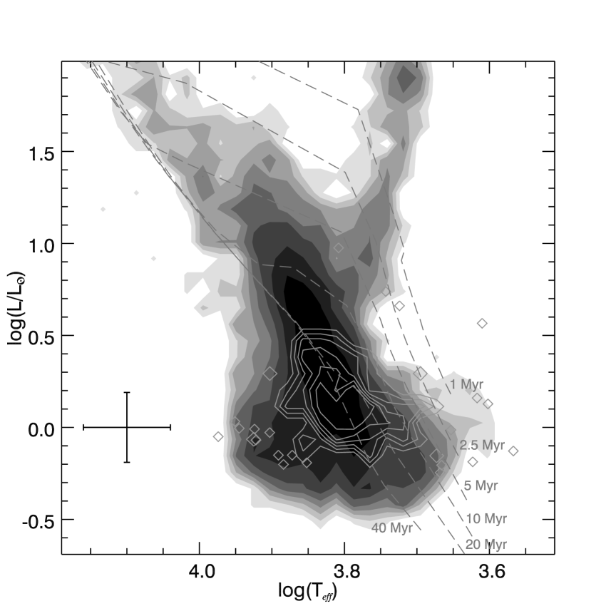
Figure 12: Hess diagram for the general population in the South field (greyscale) and the the 366 stars with unambiguous $\mathrm{H}\alpha$ emission in the South field ($(m_{\mathrm{F675W}}-m_{\mathrm{F656N}})>0.5$, contours and diamond symbols to indicate the position of individual emitters). Luminosity and temperature for the emission-line objects are computed excluding the magnitude in the F300W filter, as it can be contaminated by non-photospheric emission. Pre-Main Sequence isochrones for various ages as computed by Siess et al (siess97 (1997)) and the typical errorbar at the luminosity of the emission-line stars are also shown.

The comparison with Pre-Main Sequence isochrones by Siess et al (siess97 (1997)) shown in Figure 12 confirms the presence of a generation of young stars also among the low mass stars (the evolutionary tracks indicate masses between 0.8 and 2 $M_{\sun}$ for them). The brightest and coolest among them could be as young as 1-2 Myr, in agreement with what the upper Main Sequence indicates.

However, the majority of the emission objects seem to have ages in excess of 10 Myr. A fraction of the emission objects even falls below the locus of the Zero Age Main Sequence, a fact that, if taken at face value, would be incompatible with their suggested Pre-Main Sequence nature. Nonetheless, let us note that: (a) the observed spread in the HR diagram is consistent with being due to photometric and dereddening errors (cfr the errorbar in Figure 12), and (b) the stars with $\mathrm{H}\alpha$ excess are, on average, colder than the stars at comparable luminosity, as expected for Pre-Main Sequence objects. This is shown in Figure 13, where the temperature distribution for the candidate Pre-Main Sequence stars (solid line) is compared to the one of all of the stars (dashed line) in two intervals of luminosity (see Figure 12): $-0.2\lesssim\log(L/L_{\sun})\lesssim 0.15$ (panel (a)) and $0.15\lesssim\log(L/L_{\sun})\lesssim 0.5$ (panel (b)). Applying the Kolmogorov-Smirnov (KS) test on the unbinned data and the $\chi^{2}$ statistics to the binned data confirm that the distribution are conclusively different. In fact, the KS probability that the $\mathrm{H}\alpha$ and non-$\mathrm{H}\alpha$ emitters are drawn from the same parent distribution is less than 1.8% for the brighter sample (panel (a)) and less than 0.04% for the fainter one (panel (b)). Similarly, the deviations of the binned data correspond to $\chi^{2}$ values of 16.7 and 36.5, respectively.

Figure 13: Temperature distribution of the stars for which the $\mathrm{H}\alpha$ emission can be identified without ambiguity (solid line) compared to the one of all of the stars (dashed line) in two intervals of luminosity (see Figure 12): $-0.2\lesssim\log(L/L_{\sun})\lesssim 0.15$ (panel (a)) and $0.15\lesssim\log(L/L_{\sun})\lesssim 0.5$ (panel (b)). The Kolmogorov-Smirnov test on the unbinned data confirms that the distributions in each panel are different, with the one for the $\mathrm{H}\alpha$ emitters skewed towards lower temperature, as expected for Pre-Main Sequence stars.

Taken at face value, the old ages inferred for the candidate Pre-Main Sequence stars are at odds with the age of the brightest stars on the upper Main Sequence stars ($\sim 5$ Myr, see section 3.2). However, at this stage, we cannot claim that this age difference is real and that star formation in this field has proceeded on different timescale for different mass ranges. In fact, a shift of about 10% in temperature, in the sense of making the candidate Pre-Main Sequence stars colder, is all that it is needed to reconcile the two age determinations. Such a shift cannot be ruled out on accounts of the uncertainties in determining the stellar parameters from optical bands alone (see the discussion in Romaniello et al rom02 (2002)). Let us also note that a younger age for the candidate Pre-Main Sequence stars would also help to reconcile them with the current understanding of Galactic star-forming regions, where evidences of accretion tend to disappear in most Pre-Main Sequence stars after about 10 Myr (e.g. Calvet et al cal05 (2005), but see Romaniello et al rom04 (2004) for evidence in the LMC of vigorous accretion at an age of about 14 Myr).

Converting the measured Balmer continuum excesses described in section 3.3.2 to a mass accretion rate following the prescription of Gullbring et al (gul98 (1998), see also Robberto et al rob04 (2004)), one gets values from several times $10^{-8}$ up to $10^{-7}M_{\sun}\ \mathrm{yr}^{-1}$. If sustained for significantly longer than 10 Myr, accretion rates of this magnitude imply an accreted mass which is a large fraction of the total mass of the star and, in turn, a large mass of the circumstellar disk. To this end, a younger age for the candidate pre-Main Sequence stars would also reconcile our data with the typical disks observed in the Galaxy (a few percent of the stellar mass, e.g. Beckwith bec99 (1999) and references therein).

In this respect, however, one should also notice that the accretion rates inferred here are affected by an obvious selection effect, in that only the strongest excesses, those above the observational threshold, are detected. In addition, accreting T Tauri stars are known to exhibit temporal variation in their spectral features (e.g. Herbst et al her94 (1994, 2002)). At any given time, then, only the highest-accreting stars are detected and integrating the measured value over the lifetime of the star may lead to a gross overestimate of the total accreted mass.

3.5 The properties of the young population

Having made the case for the Pre-Main Sequence nature of the $\mathrm{H}\alpha$ and Balmer continuum excess stars, in the next two sections we will derive global properties of the young population in the South field.

3.5.1 Spatial distribution of stars

Let us now investigate the spatial distribution of the stars in the field. Since there is no obvious clustering of stars, we have simply divided the field in four regions, coinciding with the four chips of the WFPC2.

As discussed above, in order to study their spatial distribution, Pre-Main Sequence stars need to be identified on an individual basis, not just in a statistical sense. Hence, here we will consider only those objects with $(m_{\mathrm{F675W}}-m_{\mathrm{F656N}})>0.5$. The spatial distributions of massive and Pre-Main Sequence stars belonging to the same generation are shown in Figure 14. The actual numbers are reported in Table 5 together with the one of Red Clump stars, which are excellent tracers of the older field population with ages in excess of a few hundred million years (e.g. Faulkner & Cannon fau73 (1973)).

Figure 14: South Field: spatial distributions of massive ($M\gtrsim 6\leavevmode\nobreak\ M_{\sun}$; star symbol) and Pre-Main Sequence ($M\lesssim 2\leavevmode\nobreak\ M_{\sun}$; open squares) stars belonging to the same young generation. As in Table 5, the Pre-Main Sequence stars included here are only those that can be identified individually, i.e. those with $(m_{\mathrm{F675W}}-m_{\mathrm{F656N}})>0.5$. It appears that the density of hot, massive stars is significantly higher in WF2 and WF3 than elsewhere.

Chip	Massive stars	PMS	Red Clump
PC	$2\pm 1.4$	$6\pm 2.4$	$25\pm 5$
(PC$\rightarrow$WFa	$9.7\pm 6.8$	$28.8\pm 11.8$	$121\pm 24$)
WF2	$24\pm 4.9$	$100\pm 10$	$63\pm 7.9$
WF3	$29\pm 5.4$	$137\pm 11.7$	$61\pm 7.8$
WF4	$9\pm 3$	$123\pm 11.1$	$51\pm 7.1$
Total	$64\pm 8$	$366\pm 19.1$	$200\pm 14.1$
(Total$\rightarrow$WFb	$19.9\pm 2.5$	$114.4\pm 6.0$	$62.3\pm 4.4$)

Table 5: Spatial distribution of different types of stars in the four chips of the South field. The Pre-Main Sequence stars included here are only those that can be identified individually, i.e. those with $(m_{\mathrm{F675W}}-m_{\mathrm{F656N}})>0.5$. For typographical convenience we report the Poissonian uncertainty as the square root of the observed number of stars in each bin.

Most of the massive stars are confined to the WF2 and WF3 chips, i.e. in the direction of NGC 2050 (see Figure 1), whereas there is a clear deficiency of them in the PC and WF4 chips. An inspection to Figure 1 shows that the distribution of stars is, indeed, very patchy throughout the entire region and that the South field happens to be in one of the densest spots. Interestingly, the distribution of hot stars does not seem to correlate with the reddening distribution. The number of massive stars is almost the same in the WF2 and WF3 chips, but the extinction is appreciably higher in the former than in the latter (see Figure 4 and Table 3), as if the massive stars in the WF2 chip had not yet dissipated the cloud they were born from. As a word of caution, however, let us notice that our method to determine the interstellar extinction does not allow one to measure the total column density of dust along a line of sight, but, rather, the one to the star that is used as a beacon. Therefore it is possible that the true dust distribution is rather uniform across the two chips, but that stars in the “more reddened” one are just more embedded in the dust cloud. The fact that the dispersions in $\mathrm{E}(\mathrm{B}-\mathrm{V})$ are higher where the mean reddening is higher seems to favour this scenario (see Table 3).

Let us note that the number of low mass Pre-Main Sequence stars we identify through their strong $\mathrm{H}\alpha$ excess is only a lower limit to their true number. Nevertheless, the spatial distribution of the detected stars can be taken as representative of the total one. The distribution of young low mass stars belonging to the same generation as the massive ones is remarkably constant throughout the field, with the exception of the small area covered by the PC chip. As a consequence, the ratio of low-mass to massive stars is higher where the density of massive stars is lower. This is the same trend as Panagia et al (pan00 (2000)) found in the field of SN1987A and, as we will see, it is also the case in the West field. Our results, then, provide further evidence for the existence of an anti-correlation between high and low mass young stars, which indicates that star formation processes for different ranges of stellar masses are rather different and/or require different initial conditions

The density of Red Clump stars, which trace the field population with ages in excess of a few hundred million years (e.g. Faulkner & Cannon fau73 (1973)), is constant over the three WF chips and it is only marginally higher in the PC chip. Their density in the South field is virtually identical to the value measured in the West one and around SN1987A (Panagia et al pan00 (2000)). This further confirms that the older LMC population is uniformly distributed, at least on the scale of about 100 pc as probed by these three fields.

3.5.2 The mass function and star formation density

On the basis of their positions on the HR diagram, we can estimate fairly accurate masses for the most luminous stars. However, the individual masses of lower luminosity stars of the young generation are hard to determine because, taken individually, their displacements from the MS are comparable to the uncertainties of their effective temperatures and luminosities. Therefore, in a discussion of the Initial Mass Function (IMF), we have to limit ourselves to comparing the number of stars contained over quite large bins of masses. In particular, we have 64 stars with $6<M/M_{\sun}<40$ and the 781 stars with masses between 0.8 and 2 $M_{\sun}$ identified through their $\mathrm{H}\alpha$ excess. Their ratio is consistent with a mass function with a power-law slope $\alpha=-2.37$, which is indistinguishable from the “benchmark” Salpeter (salp55 (1955)) value of $\alpha=-2.35$.

This result, however, is affected by three sources of incompleteness that may make the true slope of the stellar mass function considerably different from the observed one: (1) First, our WFPC2 field is at the outskirts of a concentration of massive stars (NGC 2050, see Figure 1) and any mass segregation toward the center of the cluster could reduce the number of massive stars as compared to the one of low mass stars, making the observed slope steeper than the actual one. (2) Second, we can only identify low mass stars showing strong $\mathrm{H}\alpha$ emission that, in Galactic star-forming regions, are only a fraction of the total number of low mass Pre-Main Sequence stars. Judging from the results of the West field (see section 4), this is a function of the depth of the $\mathrm{H}\alpha$ images and can lead to an underestimate of the true number of Pre-Main Sequence stars by a factor of two. As a consequence, we can only give a lower limit to the true mass function slope. (3) Third, Pre-Main Sequence stars are intrinsically variable (see, for example Bertout bert89 (1989)) and their true number is presumably greater, possibly as much as another factor of 2, than the one determined at any given time. Again, this makes the observed mass function shallower than the true one. For example, if the true number of Pre-Main Sequence stars were $2\times 2$ greater than our direct estimate, the slope of the mass function would become $\alpha=-3$.

The total mass associated to the most recent episode of star formation can also be estimated, but it will be affected by an even larger uncertainty because, in addition to a possibly incomplete count of stars in the range 0.8-2 $M_{\sun}$, we have to extrapolate down to an unknown lower mass limit. The lowest value of the total mass is obtained adopting a relatively high value for the lower mass limit ($0.5\leavevmode\nobreak\ M_{\sun}$, Kroupa kro02 (2002)) and our derived value of the IMF of $\alpha=-2.37$. Thus we obtain a total mass of about $3,100\leavevmode\nobreak\ M_{\sun}$. Conversely, using a more canonical lower mass limit of $0.1\leavevmode\nobreak\ M_{\sun}$ and the high slope estimated above, $\alpha=-3$, the total mass of the young population would be much larger: $47,000\leavevmode\nobreak\ M_{\sun}$. Considering that these are quite extreme values and that the truth is likely to lie in the middle, we can conclude that the total mass is likely to be $12,000\leavevmode\nobreak\ M_{\sun}$, to within a factor of two (1$\sigma$).

Stars of the young generations were formed over a period of time of the order of 20 Myr. Therefore, the star formation density in this field turns out to be $0.4\leavevmode\nobreak\ M_{\sun}\mathrm{yr}^{-1}\mathrm{kpc}^{-2}$. This value is intermediate between the typical values found in actively star-forming spiral disks (up to $0.1\leavevmode\nobreak\ M_{\sun}\mathrm{yr}^{-1}\mathrm{kpc}^{-2}$) and starburst regions ($1\leavevmode\nobreak\ M_{\sun}\mathrm{yr}^{-1}\mathrm{kpc}^{-2}$ or higher, see, e.g. Table 1 of Kennicutt ken98 (1998)). We note that, while the star formation activity in the South field is rather high, still it is a couple orders of magnitude lower than in 30 Doradus also in the LMC ($100\leavevmode\nobreak\ M_{\sun}\mathrm{yr}^{-1}\mathrm{kpc}^{-2}$ in the central 10 pc, Kennicutt ken98 (1998)), the most luminous complex in the Local Group.

4 The West field

The log of the observations of the West field is reported in Table 2. Regrettably, the wide band imaging for this field is limited to two filters, and, therefore, the discussion will necessarily be more limited than in the case of the South field.

In the West field we have detected 7,978 stars down to $m_{\mathrm{F675W}}\simeq 24$, 3,416 of which have a mean error in the two available broadband filters smaller than 0.1 mag:

$$\bar{\delta}_{2}=\sqrt{\frac{\delta{{}_{\mathrm{F547W}}^{2}}+\delta{{}_{\mathrm{F675W}}^{2}}}{2}}<0.1$$ (2)

This condition, in turn, corresponds to $m_{\mathrm{F675W}}\lesssim 23$. The Colour-Magnitude diagram for the F547M (V-band like) and F675W (R-band like) filters is shown in Figure 15.

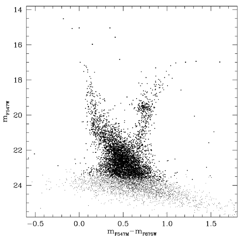
Figure 15: $m_{\mathrm{F547M}}$ vs ($m_{\mathrm{F547M}}-m_{\mathrm{F675W}}$) Colour-Magnitude diagram of the 7,978 stars detected in the West field. The black dots are the 3,416 stars with a mean photometric error in the two bands ($\bar{\delta}_{2}$, see equation 2) smaller than 0.1 mag.

A visual inspection to the diagram immediately shows the presence of different generations of stars, covering a wide age range. In particular, the brightest Main-Sequence stars (about $10\leavevmode\nobreak\ M_{\sun}$) hint to an age of 20 Myr or lower for the younger population (see below). As in the case of the South field, the presence of an old population is revealed by the Red Clump, located at $m_{\mathrm{F547M}}\simeq 19.5$, $(m_{\mathrm{F547M}}-m_{\mathrm{F675W}})\simeq$0.75, and of a well developed Red Giant Branch extending up to $m_{\mathrm{F547M}}\simeq 17$ and $(m_{\mathrm{F547M}}-m_{\mathrm{F675W}})\simeq 1$.

4.1 Reddening and ages

Since the West field was imaged only in two broad bands, we cannot recover reddening, effective temperature and luminosities for the individual stars as we did for the South field in section 3.1. However, we can still estimate the average reddening by fitting prominent features in the CMD such as the Main Sequence of the young population and the Red Clump. Using a distance modulus of $18.57\pm 0.05$ (Romaniello et al rom00 (2000)), a mean value of $\mathrm{E}(\mathrm{B}-\mathrm{V})=0.25$ for the whole field provides a good fit to the location of both features (see Figure 16).

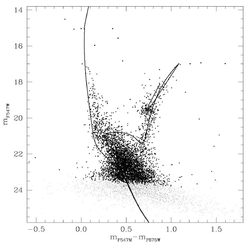
Figure 16: Same as Figure 15, but with the isochrones for 20 Myr and 5 Gyrs (Z=Z_☉/3) overplotted to the data. The isochrones have been adapted to the WFPC2 bands from the models of Brocato & Castellani (bc93 (1993)) and Cassisi et al (ccs94 (1993)) with the model atmospheres by Bessell et al (bes98 (1998)). A distance modulus of 18.57 was used (Romaniello et al rom00 (2000)), yielding an average reddening of $\mathrm{E}(\mathrm{B}-\mathrm{V})=0.25$.

In addition, Figure 16 shows that the Main Sequence is rather broad, $\delta(m_{\mathrm{F547M}}-m_{\mathrm{F675W}})\simeq 0.2$ at $m_{\mathrm{F547M}}\simeq 20$, reflecting the combined effect of differential reddening and age spread. The location of the most luminous, hence youngest, Main Sequence stars indicates an upper limit of 20 Myr to their age (regrettably, the very bluest star at $(m_{\mathrm{F547M}}-m_{\mathrm{F675W}})\simeq-0.2$ is so heavily saturated that its colour is unreliable).

The old population is composed of a mix of stars with ages from several hundred millions to several billions of years. A representative isochrone of 5 Gyr is shown in Figure 16.

4.2 Pre-Main Sequence stars

Applying the criteria discussed in section 3.4 we have identified $761\pm 37$ stars with a statistically significant $\mathrm{H}\alpha$ emission (see Figure 17). Since in the West field there are only two broad bands available, we could not recover the effective temperature for the stars. Hence, the expected $\mathrm{H}\alpha$ distribution was computed using the relation from the Kurucz (kur93 (1993)) models between the only broad-band colour we have, $(m_{\mathrm{F547M,0}}-m_{\mathrm{F675W,0}})$, and $(m_{\mathrm{F675W}}-m_{\mathrm{F656N}})$. As it can be seen in Figure 17, also in the West field stars with $(m_{\mathrm{F675W}}-m_{\mathrm{F656N}})>0.5$ can be identified individually as $\mathrm{H}\alpha$-emitting objects (264, 35% of the total of stars with a statistically significant $\mathrm{H}\alpha$ excess).

Figure 17: As in Figure 7, but for the stars in the West field. Also here, the presence of a prominent population of stars with significant $\mathrm{H}\alpha$ excess is evident. The value of the excess above which stars can be identified individually is marked with a vertical line.

It is worth noting that, even if the West field represents a sparser environment than the South field (1.6 times less stars detected in the former than in the latter), the number of $\mathrm{H}\alpha$-excess objects detected is essentially the same in the two fields ($N(\mathrm{South})=781$, $N(\mathrm{West})=761$). This is because the $\mathrm{H}\alpha$ exposures of the West field are much deeper than the ones of the South field (a factor of 2.4 in exposure time, see Tables 1 and 2). In fact, if we increase the $\mathrm{H}\alpha$ photometric errors in the West field by a factor of $\sqrt{2.4}\simeq 1.5$ to make them comparable to the ones in the South field, our procedure would identify only 210 candidate Pre-Main Sequence stars. This result provides an estimate of the uncertainties inherent in the study of an elusive population such as the one of low-mass Pre-Main Sequence stars when they are outnumbered by a much older field population.

The spatial distributions of low mass Pre-Main Sequence and massive stars in the West field are compared with each other in Figure 18 and Table 6 (the Pre-Main Sequence stars are the 264 that can be identified on an individual basis, i.e. $(m_{\mathrm{F675W}}-m_{\mathrm{F656N}})>0.5$).

Figure 18: West field: spatial distributions of massive ($M\gtrsim 6\leavevmode\nobreak\ M_{\sun}$; star symbol) and Pre-Main Sequence ($M\lesssim 2\leavevmode\nobreak\ M_{\sun}$; open squares) stars belonging to the same young generation. As in Table 6, the Pre-Main Sequence stars included here are only those that can be identified individually, i.e. those with $(m_{\mathrm{F675W}}-m_{\mathrm{F656N}})>0.5$. It is clear that the candidate Pre-Main Sequence stars are mainly concentrated in the WF3 and WF4 chips, i.e. in the direction of SN1987A (see Figure 1).

Chip	Massive stars	PMS	Red Clump
PC	$0\pm 1$	$10\pm 3.2$	$8\pm 2.8$
(PC$\rightarrow$WFa	$0\pm 1$	$48\pm 15.4$	$38.7\pm 13.6$)
WF2	$3\pm 1.7$	$66\pm 8.1$	$49\pm 7$
WF3	$4\pm 2$	$100\pm 10$	$54\pm 7.3$
WF4	$2\pm 1.4$	$88\pm 9.4$	$55\pm 7.4$
Total	$9\pm 3$	$264\pm 16.2$	$166\pm 12.9$
(Total$\rightarrow$WFb	$2.8\pm 0.9$	$82.5\pm 5.1$	$51.7\pm 4.0$)

Table 6: Spatial distribution of different types of stars in the four chips of the West field. The Pre-Main Sequence stars included here are only those that can be identified individually, i.e. those with $(m_{\mathrm{F675W}}-m_{\mathrm{F656N}})>0.5$.

Just as in the case of the South field and the region of SN1987A (Panagia et al pan00 (2000)), the ratio between low and and high-mass stars of the same generation exhibits substantial spatial variations (from 44 in the WF4 chip to roughly half of this value in the WF2 and WF3 chips) mostly due to the variations of the number of PMS among the various chips.

4.3 The mass function and star formation density

From Table 5 we see that there are 9 stars with masses between 6 and $10\leavevmode\nobreak\ M_{\sun}$ and, as discussed in the previous section, a total of 761 candidate Pre-Main Sequence stars. These numbers are consistent with a mass function slope of $\alpha\simeq-3.1$.

The same discussion presented in section 3.5.2 can be repeated for the West field. However, here incompleteness is much less of a problem, both for massive stars because there is no sign of a cluster or group of early type stars near this field (see Figure 1), nor for low-mass PMS stars because for the West field we have much deeper $\mathrm{H}\alpha$ exposures.

Thus, adopting a slope $\alpha=-3.1$, and normalising the mass function to the number of massive stars present in the field we estimate a total mass of recently formed stars between $\sim 2,300\leavevmode\nobreak\ M_{\sun}$ and $14,000\leavevmode\nobreak\ M_{\sun}$, depending on whether we assume a lower mass cutoff of 0.5 or $0.1\leavevmode\nobreak\ M_{\sun}$, respectively.

Taking the geometric mean of the two extremes as a “most probable” value of the total mass, $M_{\mathrm{tot}}=5,700\leavevmode\nobreak\ M_{\sun}$, and a formation time interval comparable to the young star ages, i.e. $\sim 20$ Myr, the star formation density in the West field turns out to be $0.2\leavevmode\nobreak\ M_{\sun}\mathrm{yr}^{-1}\mathrm{kpc}^{-2}$.

5 Summary and conclusion

In this paper we have presented HST-WFPC2 broad and narrow band imaging of two fields with recent star formation activity in the Tarantula region of the Large Magellanic Cloud. By means of the technique pioneered by Romaniello (rom98 (1998), see also Panagia et al pan00 (2000) and Romaniello et al rom04 (2004)), we have identified stars stars of 1-2 $M_{\sun}$ with a significant $\mathrm{H}\alpha$ emission: $781\pm 33$ in the South field and $761\pm 37$ in the West one. The $\mathrm{H}\alpha$ emission positively correlates with Balmer continuum excess, indicating a common physical origin for the two phenomena. The measured $\mathrm{H}\alpha$ equivalent widths (up to several tens of Å; see Figure 9) are far larger than it can be accounted for by normal chromospheric activity (e.g. Frasca & Catalano fra94 (1994), White & Basri whi03 (2003)).

Given the presence of massive young stars in both fields and the observed correlation between $\mathrm{H}\alpha$ and Balmer continuun excesses , we interpret the emission objects as Pre-Main Sequence stars. In this respect, then, they are the equivalent of the Classical TTauri stars observed in Galactic star-forming regions.

The inherent uncertainty in identifying the Pre-Main Sequence stars does not allow a precise determination of the mass function of the young population. We have discussed the different effects that bias its determination and placed a firm lower limit to its slope based solely on $\mathrm{H}\alpha$-excess stars of $\alpha=-2.37$ and $-3.1$ in the South and West field, respectively. The real mass function could be steeper should the selection criterion we have adopted miss a significant number of stars.

Also the determination of the star formation rate associated with the young generation of stars is affected by the selection criteria applied to identify the candidate Pre-Main Sequence stars, with variations of a factor of a few. Our best estimates for the star formation density are of $\sim 0.4\leavevmode\nobreak\ M_{\sun}\mathrm{yr}^{-1}\mathrm{kpc}^{-2}$ in the South field and $\sim 0.2\leavevmode\nobreak\ M_{\sun}\mathrm{yr}^{-1}\mathrm{kpc}^{-2}$ in the West field. These values are intermediate between what is found for actively star-forming spiral disks (less than $0.1\leavevmode\nobreak\ M_{\sun}\mathrm{yr}^{-1}\mathrm{kpc}^{-2}$) and starbursts ($1\leavevmode\nobreak\ M_{\sun}\mathrm{yr}^{-1}\mathrm{kpc}^{-2}$ or more; Kennicutt ken98 (1998)).

The relative spatial distribution of equally young stars with different masses, however, is not affected by the bias on the selection criteria for Pre-Main Sequence stars and provides clues to the mechanisms that lead to star formation. For both fields the spatial location of the low mass Pre-Main Sequence stars does not follow the one of the massive stars of the same young age. This further confirms the results found by Panagia et al (pan00 (2000)) for the field of SN1987A, also is in the Tarantula region (see Figure 1). The almost anti-correlation of spatial distributions of high and low mass stars of a coeval generation indicates that star formation processes for different ranges of stellar masses are rather different and/or require different initial conditions. An important corollary of this result is that the very concept of an Initial Mass Function seems not to have validity in detail, but may rather be the result of a random process, so that it could make sense to talk about an average IMF over a suitably large area, in which all different star formation processes are concurrently operating.

Appendix A The relation between EW(H${\alpha}$) and $m(\mathrm{F675W})-m(\mathrm{F656N})$

In order to compute the relation between the colour excess $m(\mathrm{F675W})-m(\mathrm{F656N})$ and the equivalent width of the $\mathrm{H}\alpha$ line, let us begin by defining $T_{R}(\lambda)$ as the total response of the system in the broad-band filter R (telescope+filter+detector) and $f(\lambda)=f_{c}+f_{l}(\lambda)$ the total flux from the source (continuum+line emission). If the continnum is assumed to be flat across the broad band, the detected flux in it is:

$$f_{R} = \int_{R}T_{R}(\lambda)f(\lambda)d\lambda=$$

$$= f_{c}\int_{R}T_{R}(\lambda)d\lambda+T_{R}(\mathrm{H}\alpha)\int_{R}f_{l}(\lambda)d\lambda$$

where we have further assumed the line to be much narrower than the filter response curve across it so that, in the last term, this latter quantity can be replaced with its value at the central wavelength of the line, $T_{R}(\mathrm{H}\alpha)$. From the definition of equivalent width (EW), it follows that:

$$\int_{R}f_{l}(\lambda)d\lambda=\mathrm{EW(\mathrm{H}\alpha)}\cdot f_{c}$$

and, hence:

$$f_{R}=f_{c}\int_{R}T_{R}(\lambda)d\lambda+T_{R}(\mathrm{H}\alpha)\cdot f_{c}\cdot\mathrm{EW(\mathrm{H}\alpha)}$$ (3)

A similar equation holds for the measured flux in the $\mathrm{H}\alpha$ narrow-band filter:

$$f_{\mathrm{H}\alpha}=f_{c}\int_{\mathrm{H}\alpha}T_{\mathrm{H}\alpha}(\lambda)d\lambda+T_{\mathrm{H}\alpha}(\mathrm{H}\alpha)\cdot f_{c}\cdot\mathrm{EW(\mathrm{H}\alpha)}$$ (4)

where $T_{\mathrm{H}\alpha}(\lambda)$ is the response curve of the narrow band filter.

Finally, transforming fluxes to magnitudes leads to the relation we are looking for, although in an implicit form:

$$m_{\mathrm{R}}-m_{\mathrm{H}\alpha}=-2.5\log(f_{R}/f_{\mathrm{H}\alpha})+\Delta(ZP)$$ (5)

where $\Delta(ZP)$ is the difference between the instrumental zero points in the broad and narrow band. In our case, we have used the WFPC2 filters F675W as R and F656N as $\mathrm{H}\alpha$ and $\Delta(ZP)=4.312$ (Whitmore whit95 (1995)).

The magnitude difference $(m_{\mathrm{F675W}}-m_{\mathrm{F656N}})$ as a function of the $\mathrm{H}\alpha$ equivalent width as computed by combining equations (3), (4) and (5) is shown in Figure 19.

Figure 19: Colour excess $m_{\mathrm{F675W}}-m_{\mathrm{F656N}}$ as a function of the $\mathrm{H}\alpha$ equivalent width computed from equations (3), (4) and (5).

- (1) Ardeberg A., Brunet J.P., Maurice E., & Prevot L. 1972, A&AS, 6, 249.
- (2) Beckwith, S.V.W. 1999, in The Origin of Stars and Planetary Systems, eds. C.J. Lada and N.D. Kylafis (Dordrecht: Kluwer Academic Publishers), 579
- (3) Bertout, C. 1989, ARA&A, 27, 351.
- (4) Bessell, M.S. 1991, A&A, 242, L17.
- (5) Bessell, M.S., Castelli, F., & Plez, B. 1998, A&A, 333, 231 (erratum 337, 321).
- (6) Brocato, E., & Castellani, V. 1993, ApJ, 410, 99.
- (7) Calvet, N., Hartmann, L., & Strom, S.E. 2002, in Protostars and Planets IV, ed. V. Mannings, A.P. Boss, & S.S. Russell (Tucson: Univ. Arizona Press), 377.
- (8) Calvet, N., Briceño, C., Hernández, J. et al, AJ, 129, 935.
- (9) Cassisi, S., Castellani, V., & Straniero, O. 1994, A&A, 282, 753.
- (10) Cool, A.M, & King, I.R. 1995, in Calibrating HST: Post Servicing Mission, eds. A. Koratkar and C. Leitherer (Baltimore: STScI), 290.
- (11) Conover, W.J. 1980, “Practical Nonparametric Statistics”, edition, (New York:Wiley).
- (12) de Wit, W.J., Beaulieu, J.P., & Lamers, H.J.L.M. 2002, A&A, 395, 829.
- (13) de Wit, W.J., Beaulieu, J.P., Lamers, H.J.L.M., Coutures, C., & Meeus, G. 2005, A&A, 432, 619.
- (14) Faulkner, D.J., & Cannon, R.D. 1973, ApJ, 180, 435.
- (15) Fernández, M., Ortiz, E., Eiroa, C., & Miranda, L.F. 1995, A&AS, 114, 439.
- (16) Fitzpatrick, E.L. 1988, ApJ, 335, 703.
- (17) Frasca, A., & Catalano, S. 1994, A&A, 284, 883.
- (18) Gilliland, R.L. 1994, ApJ, 435, L63.
- (19) Gilmozzi, R. 1990, Core Aperture Photometry with the WFPC, STScI Instrum. Rep. WFPC-90-96 (Baltimore: STScI).
- (20) Gilmozzi, R., Kinney, E.K., Ewald, S.P., Panagia, N., Romaniello, M. 1994, ApJ, 435, L43.
- (21) Gullbring, E., Hartmann, L., Briceno, C., & Calvet, N. 1998, ApJ, 492, 323.
- (22) Heyer, I., Biretta, J. et al. 2004, WFPC2 Instrument Handbook, Version 9.0 (Baltimore: STScI).
- (23) Kennicutt, R.C. 1998, ARA&A, 36,189.
- (24) Kroupa, P. 2002, Science, 295, 82.
- (25) Kurucz, R.L. 1993, ATLAS9 Stellar Model Atmosperes Programs and grid (Kurucz CD-ROM No.13).
- (26) Lamers, H.J.G.L.M., Beaulieu, J. P., & de Wit, W. J. 1999, A&A, 341, 827.
- (27) Herbst, W., Herbst, D.K., & Grossman, E.J. 1994 AJ, 108, 1906.
- (28) Herbst, W, Bailer-Jones, C.A.L., Mundt, R., Meisenheimer, K., & Wackermann, R. 2002, A&A, 396, 513.
- (29) Hodge, P.W. 1988, PASP, 100, 1051.
- (30) Madau, P., Ferguson, H.C., Dickinson, M.E., et al 1996, MNRAS, 283, 1388.
- (31) Massey, P., Johnson, K.E., & Degioia-Eastwood, K. 1995, ApJ, 454, 151.
- (32) Mateo, M. 1988, ApJ, 331, 261.
- (33) Padgett, D.L. 1996, AJ, 471, 874.
- (34) Palla, F., & Stahler, S. 1991, ApJ, 360, 47.
- (35) Panagia, N., Romaniello, M., Scuderi, S., & Kirshner, R.P. 2000, ApJ, 539, 197 (Paper I).
- (36) Pei, Y.C., Fall, S.M., & Hauser, M.G. 1999, ApJ, 522, 604.
- (37) Robberto, M., Song, J., Mora Carrillo, G., Beckwith, S.V.W., Makidon, R.B., & Panagia, N. ApJ, 606, 952.
- (38) Romaniello, M. 1998, Ph.D. Thesis, Scuola Normale Superiore, Pisa.
- (39) Romaniello, M., Salaris, M., Cassisi, S., & Panagia, N. 2000, ApJ, 530, 738.
- (40) Romaniello, M., Panagia, N., Scuderi, S., & Kirshner, R.P. 2002, AJ, 123, 91.
- (41) Romaniello, M., Robberto, M., & Panagia, N. 2004, ApJ, 608, 220.
- (42) Salpeter, E.E. 1955, ApJ, 121, 161.
- (43) Sanduleak, N. 1969, Contr. Cerro Tololo Interam. Obs, No. 89.
- (44) Schaerer, D., Meynet, G., Maeder, A., & Schaller, G. 1993, A&AS, 98, 523.
- (45) Schmidt-Kaler, T. 1982, in Landolt-Bornstein: Numerical Data and Functional Relationships in Science and Technology, vloume 2b (Berlin:Springer-Verlag), 297.
- (46) Schwering, P.B.W., & Israel, F.P. 1991, A&A, 246, 231.
- (47) Scuderi, S., Panagia, N., Gilmozzi, R., Challis, P.M., Kirshner, R.P., 1996, ApJ, 465, 956.
- (48) Siess L., Forestini M., & Dougados, C. 1997, A&A, 324, 556.
- (49) Sirianni, M., Nota, A., Leitherer, C., De Marchi, G., & Clampin, M. 2000, ApJ, 533, 203.
- (50) van der Marel, R.P., & Cioni, M.-R.L. 2001, AJ, 122, 1807.
- (51) Wichmann, R., Schmitt, J.H.M.M. & Krautter, J. 2001, A&A, 380, L9.
- (52) White, R.J, & Basri, G. 2003, ApJ, 582, 1109.
- (53) Whitmore, B. 1995, in Calibrating Hubble Space Telescope: Post Servicing Mission, eds. A. Koratkar and C. Leitherer (Baltimore: STScI), 269.
- (54) Zaritsky, D. 1999, AJ, 118, 2824.