Partial suppression of the radial orbit instability in stellar systems

Abstract

It is well known that the simple criterion proposed originally by Polyachenko and Shukhman (1981) for the onset of the radial orbit instability, although being generally a useful tool, faces significant exceptions both on the side of mildly anisotropic systems (with some that can be proved to be unstable) and on the side of strongly anisotropic models (with some that can be shown to be stable). In this paper we address two issues: Are there processes of collisionless collapse that can lead to equilibria of the exceptional type? What is the intrinsic structural property that is responsible for the sometimes noted exceptional stability behavior? To clarify these issues, we have performed a series of simulations of collisionless collapse that start from homogeneous, highly symmetrized, cold initial conditions and, because of such special conditions, are characterized by very little mixing. For these runs, the end-states can be associated with large values of the global pressure anisotropy parameter up to $2K_{r}/K_{T}\approx 2.75$. The highly anisotropic equilibrium states thus constructed show no significant traces of radial anisotropy in their central region, with a very sharp transition to a radially anisotropic envelope occurring well inside the half-mass radius (around $0.2~{}r_{M}$). To check whether the existence of such almost perfectly isotropic “nucleus” might be responsible for the apparent suppression of the radial orbit instability, we could not resort to equilibrium models with the above characteristics and with analytically available distribution function; instead, we studied and confirmed the stability of configurations with those characteristics by initializing N-body approximate equilibria (with given density and pressure anisotropy profiles) with the help of the Jeans equations.

1 Introduction

The study of the stability of a system of which the distribution function is available in analytical form can be carried out along three different approaches: N-body simulations (e.g., see Henon 1973; Merritt & Aguilar 1985; Barnes et al. 1986; Aguilar & Merritt 1990; Allen et al. 1990; Stiavelli & Sparke 1991; and following papers), linear modal analysis (Polyachenko & Shukhman 1981; Palmer & Papaloizou 1987, 1988; Weinberg 1989, 1991, 1994; Saha 1991, 1992; Bertin et al. 1994; see also Fridman & Polyachenko 1984; Palmer 1993, and references therein), and energy principles (e.g., Sygnet et al. 1984; Kandrup & Sygnet 1985; Goodman 1988, and references therein). Spherical stellar systems with too many radial orbits have thus been found to be unstable to perturbations that break the spherical symmetry and remove the excess of kinetic energy in the radial degree of freedom (see Fridman & Polyachenko 1984 and Palmer 1993). The existence of such radial orbit instability was first investigated by Polyachenko & Shukhman (1981), who proposed an “empirical criterion” for the onset of instability ($2K_{r}/K_{T}>1.7\pm 0.25$) based on the global content of kinetic energy in the radial with respect to that in the tangential degrees of freedom. Following investigations (Barnes, 1985; Merritt & Aguilar, 1985; Aguilar & Merritt, 1990; Palmer, 1993) noted that different families of models may exhibit different anisotropy thresholds for the instability, thus widening the uncertainty interval around the value of $1.7$ suggested earlier. For example, while for the so-called $f_{\infty}$ and $f^{(\nu)}$ models a threshold value similar to that suggested by Polyachenko and Shukhman may be applicable (see Bertin & Stiavelli 1989 and Trenti & Bertin 2005, hereafter TB05), for the family of Dehnen (1993) density profiles with an Osipkov-Merritt type (Osipkov, 1979; Merritt, 1985) of anisotropy profile it has been argued that such value is as high as $\approx 2.5$ (Meza & Zamorano, 1997). On the other hand, systems with an arbitrarily small content of radial anisotropy can be unstable, although with very small growth rates (as shown by Palmer & Papaloizou (1987) by means of a linear modal analysis).

The radial orbit instability is thought to play an important role during the formation of self-gravitating structures from collisionless collapse via incomplete violent relaxation, a process that has been argued to be the main driver for the formation of elliptical galaxies (van Albada, 1982). In fact, if a system starts from sufficiently cold initial conditions (i.e. with a low initial virial ratio $u=(2K/|W|)_{t=0}\lesssim 0.15$), it collapses with stars falling in almost radially toward the center, often ending up in triaxial configurations, the origin of which is attributed to the radial orbit instability (Palmer et al., 1990; Udry, 1993; Hjorth & Madsen, 1995). In general, when such collisionless collapse leads to “realistic” final configurations, the values of pressure anisotropy achieved at the end of the collapse turn out to be consistent with the threshold value associated with the instability criterion proposed by Polyachenko and Shukhman (1981). Currently, galaxy formation is approached in the generally accepted cosmological context of hierarchical clustering (see e.g. Meza et al., 2003, and references therein), but the mechanism of incomplete violent relaxation remains an important ingredient and thus quantifying the effects of the radial orbit instability is relevant to the explanation of the observed flattening of gravitational structures in cosmological simulations (see Hopkins et al. 2005).

In this paper we present the results of some numerical experiments that are aimed at clarifying the following two issues: Are there processes of collisionless collapse able to lead to equilibria of the exceptional type, that is equilibria violating the criterion proposed by Polyachenko and Shukhman (1981)? What is the structural property that makes some models with relatively low levels of global radial anisotropy unstable and others with high levels of global radial anisotropy stable?

As to the first issue, in a set of simulations of collisionless collapse (Trenti et al. 2005, hereafter TBvA05) we have investigated the role of mixing in phase space on the relaxation of the end products of the simulations. We have thus run, for comparison, a number of experiments in which phase mixing is inefficient. These are simulations with highly symmetric initial conditions. In spite of the cold initial conditions, with $u<0.1$, and of the high level of radial anisotropy achieved in the final configurations, with $2K_{r}/K_{T}$ sometimes above $2.5$ (during the process of collapse values of $2K_{r}/K_{T}$ above $10$ are reached), the radial orbit instability did not develop. From inspection of the structure of the final products of these simulations, it appears that most likely the physical factor at the basis of the observed partial suppression of the radial orbit instability is the existence of an almost perfectly isotropic central region that is realized in these systems, which appears to be more efficient for more concentrated models. This is the clue that we consider in order to address the second issue raised above.

In fact, we note that at fixed content of global anisotropy $2K_{r}/K_{T}$, the $f^{(\nu)}$ and $f_{\infty}$ models (for which the threshold value of $2K_{r}/K_{T}$ is close to 1.7) are less isotropic locally, in their core, than similar systems with anisotropy profiles of the type introduced by Osipkov (1979) and Merritt (1985), as studied by Meza & Zamorano (1997), which in turn are less isotropic in their central regions than the equilibrium states obtained at the end of our set of simulations. In the opposite direction, we recall that the generalized polytropic spheres, with small content of global anisotropy, found to be unstable by Palmer & Papaloizou (1987) are characterized by a constant and finite local anisotropy level down to $r=0$. To confirm this picture and to study the effects on the radial orbit instability of central density and anisotropy profiles decoupled from each other, we cannot resort to equilibrium models with the above characteristics and with analytically available distribution function. We have then constructed with the help of the Jeans equations N-body equilibria with density and anisotropy profiles qualitatively similar to those found as end states for the simulations of collisionless collapse violating the criterion proposed by Polyachenko & Shukhman (1981) and thus demonstrated that some configurations with $2K_{r}/K_{T}$ up to $\approx 2.9$ do not show evidence of rapid evolution.

The paper is organized as follows. In the next Section we describe some special processes of collisionless collapse leading to highly anisotropic quasi-equilibrium states. In Sect. 3 we investigate the evolution of candidate collisionless equilibrium configurations constructed numerically starting from the Jeans equations and identify a quasi-equilibrium state with $2K_{r}/K_{T}\approx 2.9$. Conclusions are presented in Sect. 4. In the Appendix we outline the method used to generate approximate equilibrium configurations with given density and anisotropy profiles starting from the Jeans equations.

2 Exceptionally stable equilibria resulting from special processes of collisionless collapse

Most of the numerical simulations discussed in this paper have been carried out with the recently developed particle-mesh code described in TBvA05 (for further tests and details see also Trenti, 2005). The code solves the Poisson equation by expanding the density and the potential in spherical harmonics and is well suited for the study of the stability of collisionless systems (TB05). We have also run a few simulations with the fast tree code GyrFalcON (Dehnen, 2000, 2002) to check, with success, that our results are not biased by the specific choice of the numerical code.

As briefly noted in the Introduction, it is well known (see van Albada 1982 and many following papers) that the collapse of a cold cloud of stars can lead, on a dynamical time-scale, to the formation of an equilibrium structure characterized by a quasi-isotropic core and a radially anisotropic halo with projected density profiles similar to the $R^{1/4}$ law (de Vaucouleurs, 1948). The mechanism of incomplete violent relaxation (Lynden-Bell, 1967) has thus been advocated as a possible scenario for the formation of elliptical galaxies. Several investigations (van Albada, 1982; McGlynn, 1984; Londrillo et al., 1991) have shown that the outcome of the simulations generally resembles observed systems provided the initial conditions are clumpy. This condition finds a natural interpretation in the current cosmological framework for structure formation, as the use of clumpy initial conditions in collisionless collapse simulations may effectively mimic some aspects of hierarchical merging. Simulations of mergers of stellar systems, i.e. of incomplete violent relaxation, are generally considered as an important tool to study the properties of elliptical galaxies, not only in view of an explanation of the origin of the universality of the observed surface brightness profiles, but also in relation to the origin and evolution of the Fundamental Plane (Nipoti et al., 2003; González-García & van Albada, 2003). Observational evidence is now accumulating in support of the importance of mergers as a formation mechanism for elliptical galaxies (e.g. see van Dokkum & Ellis, 2003; Bell et al., 2004), although many arguments and new findings tend to point to a merger process in which dissipation plays a significant role. In addition, Khochfar & Burkert (2003) (see also Jesseit et al. 2005) argue from semi-analytic modeling that $50~{}\%$ of present days ellipticals are relics of mergers between spheroidal systems.

For the present study, we focus on a particular set of simulations that start from homogeneous spherically symmetric configurations obtained by symmetrizing a clumpy configuration with ten cold clumps, the kinetic energy of which is in the collective motion of their center of mass. In most of the runs $u=(2K/|W|)_{t=0}<0.1$; the clump radius is taken to be equal to one half of the half-mass radius of the system. The symmetrization is performed by accepting the radius and the magnitude of the velocity of each simulation particle, following the procedure to generate clumpy conditions discussed in TBvA05, and by redistributing uniformly the angular variables in both position and velocity space. This initialization procedure leads to a smooth initial density profile, decreasing approximately linearly in radius ($\rho(0)\approx 2\rho(r_{M})$), which creates a potential well that is deeper than the one of a uniform sphere with the same cutoff radius. The initial system is non-rotating and isotropic. Mild correlations in the magnitude of the velocities are present, since there is a residual memory of the cold clumpy state. The precise form of the density profile as well as the strength of the velocity correlations depend on the details of the initial random positions of the clump centers, i.e. on the seed of the random number generator.

A snapshot of typical initial conditions from which our set of simulations of collisionless collapse starts is reported in Fig. 1. The correlations in the magnitude of the velocities, characteristic of the original clumps from which the present initial conditions are extracted, can be seen as ring patterns created by the particles in the $(v_{x};v_{y})$ space. We should emphasize that these initial conditions are rather artificial and have been employed with the specific purpose of studying the effects of the suppression of mixing in phase space. It appears unlikely that in a realistic scenario of galaxy formation the initial state is characterized by such high degree of symmetry. Nevertheless, the properties of the end-products of these collapse simulations are not too unrealistic, at least in their outer parts (see Subsection 2.1).

In Table 1 we summarize the properties of this set of simulations. The initial conditions of the $S1$ series are generated using the same positions for the clump centers but a different total number of particles $N$ (to ensure that the properties of the end products do not depend on $N$). Run $S1^{+}$ has $8\times 10^{5}$ simulation particles; $S1^{*}$ and $S1^{\dagger}$ have $10^{5}$ particles, but the first simulation is run with our particle-mesh code, while the second with Dehnen’s code. Runs $Sa$ and $Sb$ are colder versions of $S1^{*}$ (obtained by means of a global rescaling of the initial velocities by a constant factor). Runs $S2$ and $S3$ are generated using a different seed for the random numbers. In order to characterize the level of anisotropy achieved in the end-states obtained from the simulations, we refer to the global anisotropy parameter $2K_{r}/K_{T}$ and to the anisotropy profile $\alpha(r)$, defined as $\alpha(r)=2-(\langle v^{2}_{\theta}\rangle+\langle v^{2}_{\phi}\rangle)/\langle v^{2}_{r}\rangle$.

During collapse, the spherical symmetry is well preserved, as can be seen for $S1$ not only from the evolution of the eigenvalues of the inertia tensor of the system (Fig. 2), but also from the conservation of the single particle angular momenta (Fig. 3). Mass loss (i.e. the number of particles that acquire a positive energy during the collapse) is limited, well below the loss recorded for homogeneous uniform spheres with similar initial virial ratio $u$, where the system can lose up to one third of its total mass. The combination of spherical symmetry and limited mass loss leads to high final density concentrations, with $\rho(0)/\rho(r_{M})\gtrsim 1500$ in run $S1$. As shown in Fig. 4, the density profile is reasonably well represented by a rather concentrated $f^{(\nu)}$ model (see TB05) or by a Jaffe density profile (Jaffe, 1983).

The global amount of pressure anisotropy (see Fig. 2) evolves rapidly in the first few dynamical times and then reaches its quasi-equilibrium value at $t\approx 5t_{d}$. When $2K_{r}/K_{T}$ reaches its peak value, at the time of maximum contraction of the system, the anisotropy radius $r_{\alpha}$ (defined implicitly by $\alpha(r_{\alpha})=1$) is located well inside: at that time, for run $S1$ the mass within $r_{\alpha}$ is only $1\%$ of the total mass, while later the sphere associated with the anisotropy radius contains approximately $20\%$ of the total mass. The final global content of pressure anisotropy is high also for run $S3$, which starts from moderately warm initial conditions ($u=0.25$; for comparison, see the results of non-symmetrized runs with phase-space mixing presented in TBvA05).

Interestingly, the central regions have a final pressure anisotropy profile slightly biased toward tangential orbits (see Fig. 4). This effect appears in the high resolution $S1^{+}$ simulation, with $8\times 10^{5}$ particles; the realization with $10^{5}$ particles ($S1^{*}$) does not exhibit this feature and indeed is characterized by a slightly higher value of $2K_{r}/K_{T}$. In any case the transition from isotropic to radial pressure is very sharp. The shape of the anisotropy profile cannot be represented either by a profile similar to those of the $f^{(\nu)}$ models or by an Osikpov-Merritt profile (Osipkov, 1979; Merritt, 1985).

To check the robustness of the numerical results, with Dehnen’s tree code we have let the final configuration reached in $S1^{*}$ evolve for $30$ additional dynamical times, without noticing any sign of significant changes. In addition, we have run a collapse simulation starting with the same initial conditions as $S1^{*}$ using Dehnen’s tree code during the entire simulation (run $S1^{\dagger}$); this simulation shows no macroscopic differences with respect to $S1^{*}$ (these are summarized in Table 1 and are at the level of $1\%$ ).

If we consider colder and colder initial conditions within the framework of simulations considered in this paper, the radial orbit instability eventually sets in. A reduction of the initial virial ratio $u$ below $0.05$ for $S1$-like initial conditions (by rescaling the velocities by a constant factor) leads to runs that show evidence for the radial orbit instability: a simulation with $u=0.03$ ($Sb$) leads to a strongly flattened system, with a final amount of global anisotropy close to $2.5$.

A simulation starting from $u=0.05$ shows an interesting behavior which we may identify as that of marginal stability, since the final state is characterized by an aspect ratio (see Fig. 5) $\eta$ that oscillates between 0.99 and 0.93, on a time scale longer than the dynamical time; the related anisotropy content is high ($2K_{r}/K_{T}\approx 2.75$).

2.1 Elliptical galaxies and the properties of the end-products of some symmetric collisionless collapse simulations

As we have seen above, the end-products of this set of simulations, starting from highly symmetric initial conditions, are characterized by a density profile which is not too far from that of models, such as the Jaffe (1983) profile, that are known to be associated with realistic surface brightness profiles for bright elliptical galaxies (under the assumption of constant mass-to-light ratio). To quantify the effects of the systematic differences between these models and the products of the simulations, in Fig. 6 we consider the projected density profile measured at the end of simulation $S1^{+}$ and we compare it to the $R^{1/4}$ (de Vaucouleurs, 1948) and to the $R^{1/n}$ (Sersic, 1968) laws. The residuals from the best fit, at fixed effective radius $R_{e}$, are not too large, especially for the Sersic law with $n\approx 8.3$. In fact, the deviations are within $0.2$ magnitudes over a wide interval in radius, from $0.2$ to $10~{}R_{e}$; however, in the central regions the difference can be as high as $0.5$ magnitudes, probably because of the presence of the “bump” in the density profile around $0.1~{}r_{M}$ (see Fig. 4). Residuals from the $R^{1/4}$ are larger.

For a direct comparison of the models considered in this paper and the observations, one might think of making a kinematical test. Unfortunately, as to the anisotropy of the velocity dispersion tensor, at present a comparison with the observations would be extremely difficult to carry out. The best empirical evidence for radial anisotropy in elliptical galaxies comes from the observed flattening (and triaxiality) in objects that are not rotationally supported. In principle, pressure anisotropy affects the shape of the velocity distribution integrated along the line of sight, so that its presence could be detected by observing the shapes of the line profiles (and in particular the deviations from Gaussian profiles). In practice, the effects on line profiles are rather modest even for significant amounts of pressure anisotropy, so that, within the uncertainty limits of the measurement, the pressure anisotropy profile of elliptical galaxies remains basically undetermined by current observations (e.g., see Gerhard, 1993; Gerhard et al., 2001; de Zeeuw et al., 2002). In other words, it would be very hard to ascertain whether some ellipticals are indeed as isotropic in their inner regions as implied by some of the models that we have investigated.

As briefly mentioned in the Introduction, numerical simulations of galaxy formation suggest that elliptical galaxies may be close to marginal stability with respect to the radial orbit instability, close to the threshold stated by Polyachenko & Shukhman (1981). In this respect, studying the effects on the radial orbit stability of a highly isotropic core, as we do in this paper, is of interest, because there are astrophysical processes that are often ignored in the simulations of galaxy formation and should operate in real elliptical galaxies, which may favor a more isotropic core or even an anisotropic core with a slight bias of the pressure tensor in the tangential directions. Here we have in mind processes such as those due to the presence of a super-massive black hole (for the effects of a black hole on the pressure anisotropy within the sphere of influence see e.g., Cipollina & Bertin 1994, Baumgardt et al. 2004). To be sure, for a physically significant application of these ideas, one should check the time-scales of the competing processes that are invoked, before drawing the relevant conclusions.

3 Exceptionally stable equilibria constructed from the Jeans equations

We now address the issue of whether a given initial configuration, characterized by assigned density $\rho(r)$ and pressure anisotropy $\alpha(r)$ profiles, is stable with respect to the radial orbit instability. We are not aware of models with analytical distribution function able to incorporate the sharp feature in the anisotropy profile, of the kind observed at the end of the simulations described in the previous Section. Therefore, we decided to initialize the simulations by means of candidate equilibrium solutions obtained from the Jeans equations, as outlined in the Appendix. We should emphasize that the simulations that we describe below in this Section are simulations of candidate equilibria. In fact, since we never reach the point of actually reconstructing an underlying equilibrium distribution function, if we happened to find significant evolution we could be either in a situation of genuine instability, or, more simply, in a situation of non-equilibrium. In turn, since we will show cases where we do not find such evolution, we may claim that indeed we have found not only a genuine quasi-equilibrium state but also proved that it is approximately stable.

To model a density profile of the kind found at the end of the $S1$ simulations, when no evolution is observed over several dynamical times, we use a superposition of a regularized Jaffe (1983) profile:

$$\rho_{J}(r)=\frac{A}{(r^{2}+\epsilon^{2})(r+b)^{2}},$$ (1)

with $A$, $\epsilon$, and $b$ free scales, and a central core of the form:

$$\rho_{C}(r)=\frac{A^{\prime}}{(r^{2}+\xi b^{2})^{20}},$$ (2)

where $A^{\prime}$ is a free scale, while $\xi$ is a dimensionless parameter of order $1$ ($\xi\approx 0.6$). The form for the density $\rho_{mod}=\rho_{J}+\rho_{C}$ is taken for convenience, so as to reproduce not only the large-scale structure of the density distribution realized in the $S1$ simulations, but also the bump in the density profile around $r_{M}/5$ (see Fig. 4).

As noted earlier, the $S1$ anisotropy profile is flatter than the corresponding Osipkov-Merritt profile with same $r_{\alpha}$ at small radii, while it is less steep at large radii. Thus we chose to represent the profile with:

$$\alpha(r)=2\frac{r^{\gamma}}{r^{\gamma}+r_{a}^{\gamma}}$$ (3)

with $r_{a}$ and $\gamma$ being free parameters. A single choice of the $(r_{a};\gamma)$ values is unable to correctly reproduce the anisotropy profile measured from the simulation over the entire radial range. Thus we fit separately the anisotropy in the “core”, up to a radius $r_{ch}\gtrsim r_{\alpha}$, where $\gamma=4$, and in the “halo”, i.e. for $r>r_{ch}$, where $\gamma=6/5$. In a neighborhood around $r_{ch}$ the two profiles are matched so that the final $\alpha(r)$ and its derivative are continuous functions.

With a suitable choice for the various parameters that define the above functions, the profiles obtained from the simulation can be fitted with an accuracy of better than $10$ percent. We take this as a good starting point to investigate the stability of equilibrium configurations similar to those produced in the simulations of collisionless collapse.

We have first studied the evolution of a model initialized with density and anisotropy profiles similar to those of runs $S1$ (see entry $J1$ in Table 2 and Fig. 7). We have then proceeded to study the evolution of neighboring configurations by slightly modifying the density and/or the anisotropy profiles. In particular, we have considered models with a density profile without the inner “bump” (i.e., without the $\rho_{C}$ contribution), and different forms of anisotropy profile, ranging from steep profiles over the entire radial range, to Osipkov-Merritt and $f^{(\nu)}$-like profiles. Interestingly we have found that although none of the various combinations turns out to be violently unstable, nevertheless, the only simulation where practically no sign of evolution occurs is $J1$, the one associated with the profiles that best fit those of $S1$.

For the systems that show definite signs of evolution, the evolution appears to be very slow. For example, in the $J2$ simulation the initial configuration lasts basically unchanged for more than $10$ dynamical times. In this case, illustrated in Fig. 8, the system remains close to spherical symmetry with $2K_{r}/K_{T}\approx 2.9$, and ends up only much later as a prolate system.

4 Conclusions

In this paper we have studied and clarified the dependence of the radial orbit instability on the shape of the anisotropy profile in the central region of a stellar system. By means of a series of numerical simulations we have shown that stable, centrally isotropic equilibria with a significant global amount of anisotropy can be reached during highly symmetric cold collapse events or initialized by solving the Jeans equations. In particular we have found a metastable state with $2K_{r}/K_{T}\approx 2.9$.

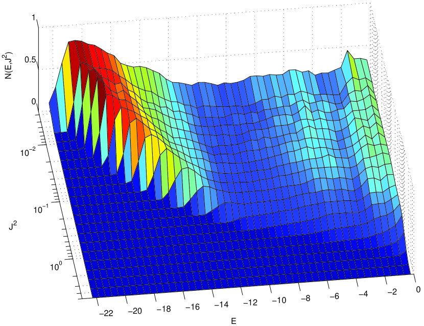
Figure 9: Phase space distributions $N(E)$ (left) and $N(E,J^{2})$ (right) for the final state reached in the $S1^{+}$ simulation. The peak in the bottom left panel around $E\approx-14$ (in code units) is associated with the isotropic core.

The experiments that we have performed suggest that the presence of an isotropic core may act as an important stabilizing factor for the radial orbit instability. The two-component (core-halo) structure for run $S1^{+}$ is indeed evident not only in the density and pressure anisotropy profiles (see the structure out to $r\approx r_{M}/5$ in Fig. 4), but also in the phase space distribution $N(E)$, as indicated by the peak located at high values of the binding energy ($E\approx-14$, in code units; see left panel of Fig. 9).

One indication for the stabilizing effect of a highly isotropic core may be found by recalling that the linear modal stability analyses have shown that the density profiles of the fastest growing modes are peaked in the innermost region of the system (see e.g., Bertin et al., 1994, Fig 8). Thus we may argue that, if the core were almost perfectly isotropic, there would be no room for the modes to be excited.

These results are qualitatively reminiscent (although the physical mechanisms that are involved are completely different), of the stabilizing role that a hot bulge can provide in relation to the stability of self-gravitating disks, as noted in a number of papers starting with Berman & Mark (1977) and Sellwood (1981). For disks, the detailed mechanisms underlying the origin or the suppression of global bar and spiral instabilities are reasonably well understood and known to depend on the key structural properties of the basic state (i.e., the disk density, effective velocity dispersion, and differential rotation profiles). For anisotropic spherical stellar systems we still lack a clear picture of the relevant underlying mechanisms. In this respect, this paper offers an interesting clue to more systematic studies that should be devoted to investigating the nature of the radial orbit instability in two-component systems, also in view of the central properties of the dark halo.

Appendix A Candidate collisionless equilibria generated by the Jeans equations

The goal is to construct stellar dynamical configurations, as initial conditions for N-body simulations, corresponding to systems with given density and pressure anisotropy profiles. As is well known, in general this problem is not well-posed, because a given pair $(\rho(r),\alpha(r))$ may even lack a physically acceptable underlying equilibrium distribution function. We proceed by applying the necessary constraints of the Jeans equations and then initialize our simulations with a procedure described below, well aware that we may actually miss the desired equilibrium conditions (see comment at the beginning of Sect. 3).

The knowledge of the density profile immediately identifies the self-consistent potential $\Phi(r)$. In addition, it defines the integrated mass profile, from which the positions of the particles can be correctly initialized. In the absence of an analytical distribution function, to complete the initialization of the N-body collisionless candidate equilibrium configuration we then resort to the Jeans equations to extract the information about the velocity dispersion profile that would be required by the conditions of equilibrium. In practice, for a non-rotating spherically symmetric system the relevant hydrostatic equilibrium equation can be written as:

$$\frac{d(\rho(r)\sigma^{2}_{r}(r))}{dr}+\frac{\rho(r)}{r}\alpha(r)\sigma^{2}_{r}(r)=-\rho(r)\frac{d\Phi(r)}{dr},$$ (A1)

where $\Phi$ represents the mean field gravitational potential (which can be taken to be known for known $\rho(r)$) and $\sigma^{2}_{r}=\langle v^{2}_{r}\rangle$ the velocity dispersion in the radial direction. For assigned profiles $(\rho(r),\alpha(r))$, under the natural boundary condition given by

$$\rho(\infty)\sigma^{2}_{r}(\infty)=0,$$ (A2)

the equation can be solved for $\sigma^{2}_{r}$:

$$\sigma^{2}_{r}(r)=\frac{1}{\rho(r)}\int_{r}^{+\infty}dr^{\prime}\frac{d\Phi(r^{\prime})}{dr^{\prime}}\rho(r^{\prime})\exp{\left\{\int_{r}^{r^{\prime}}\frac{\alpha(\tilde{r})}{\tilde{r}}d\tilde{r}\right\}}.$$ (A3)

Thus we have obtained the velocity dispersion profiles consistent with the given density and anisotropy profiles.

At this point, we initialize our N-body code by assuming that the velocity dispersion profiles obtained above correspond, at least approximately, to a truncated Gaussian distribution in velocity space (the truncation is imposed by the requirement that only bound particles, i.e. particles with negative energy, belong to the system). This assumption gives a reasonable description of systems for which the velocity distribution is determined by physically motivated distribution functions (e.g., for the stable $f^{(\nu)}$ models); but, in general, there is no guarantee that N-body systems initialized by this method be in approximate dynamical equilibrium.

In our case, the limitations of this approach are not severe, because we are interested in a stability study. If we happen to obtain a configuration with no significant signs of evolution, we are certain a posteriori that a quasi-equilibrium state has indeed been produced. On the other hand, even if the initialization gives a configuration not in dynamical equilibrium, but a nearby equilibrium configuration is approached on a very short time scale (typically on the order of one dynamical time), then we may argue that we have also obtained our goal of producing a quasi-equilibrium state with characteristics close to those desired.

A.1 Tests on known distribution functions

We have tested our method on isotropic systems by initializing Plummer and polytropic models and then on some anisotropic configurations associated with the $f^{(\nu)}$ family (see TB05), under conditions of stability. By construction, we have a good match at the level of density, velocity dispersion, and anisotropy profiles. Differences in the fourth order moment of the velocity distribution are typically at the level of a few percent. The models initialized with the method outlined above appear to be stable, except for some modest re-arrangements of the initial anisotropy profile in the case of the $f^{(\nu)}$ models. In the latter case, there is a tendency for the anisotropy content in the central region to decrease so that a flatter profile in $\alpha(r)$ is eventually generated.

Figure 1: Snapshot of the initial conditions in the planes $(x,y)$ (left panel) and $(v_{x},v_{y})$ (right panel) for simulation $S1$. The plots are given in code units. The effects of the symmetrization over the initial conditions of the kind considered in TBvA05 are easily appreciated in velocity space, where clumpiness before symmetrization was high (see Fig. 3 in TBvA05); here particles tend to form ring structures. The adopted symmetrization of initial conditions suppresses mixing in phase space during collisionless collapse.

Figure 2: Left panel: evolution of the ellipticities $\epsilon=b/a$ and $\eta=c/a$, where $a\geq b\geq c$ are the values of the axes of the system evaluated from the inertia tensor, for the $S1^{+}$ simulation. Right panel: evolution of the ratio $2K_{r}/K_{T}$ for the same simulation. The dynamical time is defined in terms of the total mass and of the total energy as $t_{d}=GM^{5/2}/(-2E_{tot})^{3/2}$.

Figure 3: Left panel: variation of one component of the specific angular momentum of the simulation particles for run $S1^{+}$. Since during evolution the system remains spherically symmetric, the single particle angular momenta are approximately conserved. Right panel: Distribution of initial angular momenta (solid line) for the same simulation: the distribution basically coincides with that for the final angular momenta (dotted line).

Figure 4: Density (in code units; left) and anisotropy profile (right) for the final state reached in the $S1^{+}$ simulation. The solid line in the left panel is the density profile associated with the $(1/2;6.4)$ $f^{(\nu)}$ model (see TB05 for definitions and notation). The anisotropy profile is compared to the Osipkov-Merritt anisotropy profile (solid line) and to the profile for an $f^{(\nu)}$ model characterized by a similar amount of global anisotropy (dashed line; the $(1/2;1)$ model, which has the same $r_{\alpha}$ as the end-state for $S1^{+}$). Clearly the theoretical models are unable to capture the rapid increase in $\alpha$ at $r\sim r_{\alpha}$.

Figure 5: Ellipticities (left) and anisotropy content (right) for the $Sa$ simulation, as plotted in Fig. 2. Note the extremely high value of anisotropy content ($2K_{r}/K_{T}>20$) reached during the collapse.

Figure 6: Residuals from the fit with the $R^{1/4}$ law (solid line) and with the $R^{1/n}$ law (dashed line), in magnitudes, of the projected density profile for the final configuration reached in simulation $S1^{+}$. The fit has been obtained by considering a constant mass-to-light ratio, at fixed effective radius $R_{e}$. The best fitting index $n$ is $n\approx 8.3$. Note the sizable residuals in the central regions.

Figure 7: Ellipticities (left) and anisotropy content (right) for the $J1$ simulation, as plotted in Fig. 2.

Figure 8: Ellipticities (left) and anisotropy content (right) for the $J2$ simulation ($2K_{r}/K_{T}=2.92$ at $t=0$), as plotted in Fig. 2.

Table 1: Collapse simulations. The simulations have been run with $N=10^{5}$ particles, except $S1^{+}$ for which $N=8\times 10^{5}$. The columns list the initial virial ratio $u=(2K/|W|)_{t=0}$, the fractional mass loss $\Delta M=[M(t=0)-M(t_{end})]/M(t=0)$, the final global anisotropy $\kappa=2K_{r}/K_{T}$ of the system of bound particles, its anisotropy radius $r_{\alpha}$ (i.e. the radius where the local anisotropy parameter is $\alpha=1$) in units of the half-mass radius, and the ellipticities $\epsilon=b/a$ and $\eta=c/a$, where $a\geqslant b\geqslant c$ are the axes of the final quasi-equilibrium state computed from the inertia tensor.

	$u$	$\Delta M$	$\kappa_{end}$	$r_{\alpha}/r_{M}$	$\epsilon$	$\eta$
$S1^{+}$	0.07	0.01	2.49	0.18	1.00	0.99
$S1^{*}$	0.07	0.01	2.54	0.18	0.99	0.98
$S1^{\dagger}$	0.07	0.01	2.52	0.18	0.98	0.97
$Sa$	0.05	0.03	2.75	0.18	0.98	0.97
$Sb$	0.03	0.07	2.56	0.16	0.79	0.66
$S2$	0.08	0.10	2.16	0.30	1.00	0.98
$S3$	0.25	0.00	2.13	0.29	0.99	0.98

Table 2: Simulation runs initialized with models constructed from the Jeans equations. The simulations have $2\times 10^{5}$ particles. Here we list the initial and final global anisotropy $\kappa=2K_{r}/K_{T}$ of the system, its final anisotropy radius in terms of the half-mass radius, and the final ellipticities $\epsilon=b/a$ and $\eta=c/a$, where $a\geqslant b\geqslant c$ are the axes evaluated from the inertia tensor. The initial conditions are summarized in the last column and range from the best fit of $S1$, simulation $J1$, to regularized Jaffe profiles $\rho_{J}$ (see Eq. 1) with Osipkov-Merritt or $f^{(\nu)}$ like anisotropy. Note that simulation $J4$, initialized with a regularized Jaffe density plus an unstable $f^{(\nu)}$ anisotropy profile ($\kappa\approx 2.3$) evolves rapidly within the first dynamical time and the anisotropy is quickly reduced below $\kappa=2$ while preserving the spherical symmetry.

	$\kappa_{0}$	$\kappa_{end}$	$r_{\alpha}/r_{M}$	$\epsilon$	$\eta$	notes:
J1	2.47	2.42	0.26	0.98	0.98	as S1
J2	2.92	2.12	0.37	0.48	0.48	$\rho_{J}+\alpha_{S1}$
J3	2.40	2.45	0.28	0.96	0.94	$\rho_{J}+\alpha_{OM}$
J4	2.29	1.93	0.61	0.99	0.99	$\rho_{J}+\alpha_{f^{(\nu)}}$
J5	2.47	2.26	0.30	0.63	0.63	$\rho_{S1}+\alpha_{OM}$

References

- Aguilar & Merritt (1990) Aguilar, L. A. and Merritt, D. 1990, ApJ, 354, 33
- Allen et al. (1990) Allen, A. J., Palmer, P. L., and Papaloizou J. 1990, MNRAS, 242, 576
- Barnes (1985) Barnes, J. 1985, in IAU Symp. 113: Dynamics of Star Clusters, Dordrecht, Reidel. pp 297–299
- Barnes et al. (1986) Barnes, J., Hut, P., and Goodman J. 1986, ApJ, 300, 112
- Baumgardt et al. (2004) Baumgardt, H., Makino, J., and Ebisuzaki T. 2004, ApJ, 613, 1133
- Bell et al. (2004) Bell, E. F. et al. 2004, ApJ, 608, 752
- Berman & Mark (1977) Berman, R. H. and Mark, J. W. K. 1977, ApJ, 216, 257
- Bertin et al. (1994) Bertin, G., Pegoraro, F. Rubini, F., and Vesperini E. 1994, ApJ, 434, 94
- Bertin & Stiavelli (1989) Bertin, G. and Stiavelli, M. 1989, ApJ, 338, 723
- Cipollina & Bertin (1994) Cipollina, M. and Bertin, G. 1994, A&A, 288, 43
- Dehnen (1993) Dehnen, W. 1993, MNRAS, 265, 250
- Dehnen (2000) Dehnen, W. 2000, ApJ, 536, L39
- Dehnen (2002) Dehnen, W. 2002, J. Comp. Phys., 179, 27
- de Vaucouleurs (1948) de Vaucouleurs, G 1948, Ann. Astr., 11, 247
- de Zeeuw et al. (2002) de Zeeuw, P. T. et al. 2002, MNRAS, 329, 513
- Fridman & Polyachenko (1984) Fridman, A. M. and Polyachenko, V. L. 1984, Physics of gravitating systems. New York: Springer
- Gerhard (1993) Gerhard, O. E. 1993, MNRAS, 265, 213
- Gerhard et al. (2001) Gerhard, O., Kronawitter, A., Saglia, R. P., and Bender, R. 2001, AJ, 121, 1936
- González-García & van Albada (2003) González-García, A. C. and van Albada, T. S. 2003, MNRAS, 342, L36
- Goodman (1988) Goodman, J. 1988, ApJ, 329, 612
- Henon (1973) Henon, M. 1973, A&A, 24, 229
- Hjorth & Madsen (1995) Hjorth, J. and Madsen, J. 1995, ApJ, 445, 55
- Hopkins et al. (2005) Hopkins, P., Bahcall, N., and Bode, P. 2005, ApJ, 618, 1
- Jaffe (1983) Jaffe, W. 1983, MNRAS, 202, 995
- Jesseit et al. (2005) Jesseit, R., Naab, T., and Burkert, A. 2005, MNRAS, 360, 1185
- Kandrup & Sygnet (1985) Kandrup, H. E. and Sygnet, J. F. 1985, ApJ, 298, 27
- Khochfar & Burkert (2003) Khochfar, S. and Burkert, A. 2003, ApJ, 597, 117
- Londrillo et al. (1991) Londrillo, P., Messina, A., & Stiavelli, M. 1991, MNRAS, 250, 54
- Lynden-Bell (1967) Lynden-Bell, D. 1967, MNRAS, 131, 101
- McGlynn (1984) McGlynn, T. A. 1984, ApJ281, 13
- Merritt (1985) Merritt, D. 1985, AJ, 90, 1027
- Merritt & Aguilar (1985) Merritt, D. and Aguilar, L. A. 1985, MNRAS, 217, 787
- Meza et al. (2003) Meza, A., Navarro, J. F., Steinmetz, M., and Eke, V. R. 2003, ApJ, 590, 619
- Meza & Zamorano (1997) Meza, A. and Zamorano, N. 1997, ApJ, 490, 136
- Osipkov (1979) Osipkov, L. P. 1979, Soviet Astronomy Letters, 5, 42
- Nipoti et al. (2003) Nipoti, C., Londrillo, P., and Ciotti, L. 2003, MNRAS, 342, 501
- Palmer (1993) Palmer, P. 1993, Stability of collisionless stellar systems. Kluwer Academic Publishers
- Palmer & Papaloizou (1987) Palmer, P. L. and Papaloizou, J. 1987, MNRAS, 224, 1043
- Palmer & Papaloizou (1988) Palmer, P. L. and Papaloizou, J. 1988, MNRAS, 231, 935
- Palmer et al. (1990) Palmer, P. L., Papaloizou, J., and Allen, A. J. 1990, MNRAS, 246, 415
- Polyachenko & Shukhman (1981) Polyachenko, V. and Shukhman, I. 1981, Soviet Ast., 25, 533
- Saha (1991) Saha, P. 1991, MNRAS, 248, 494
- Saha (1992) Saha, P. 1992, MNRAS, 254, 132
- Sellwood (1981) Sellwood, J. A. 1981, A&A, 99, 362
- Sersic (1968) Sersic, J. L. 1968, Atlas de galaxias australes, Cordoba, Argentina: Observatorio Astronomico, 1968
- Stiavelli & Sparke (1991) Stiavelli, M. and Sparke, L. S. 1991, ApJ, 382, 466
- Sygnet et al. (1984) Sygnet, J. F., des Forets, G., Lachieze-Rey, M., and Pellat, R. 1984, ApJ, 276, 737
- Trenti (2005) Trenti, M. 2005, PhD thesis, Scuola Normale Superiore, Pisa
- Trenti & Bertin (2005) Trenti, M. and Bertin, G. 2005, A&A, 429, 161 (TB05)
- Trenti et al. (2005) Trenti, M., Bertin, G., and van Albada, T. S. 2005, A&A, 433, 57 (TBvA05)
- Udry (1993) Udry, S. 1993, A&A, 268, 35
- van Albada (1982) van Albada, T. S. 1982, MNRAS, 201, 939
- van Dokkum & Ellis (2003) van Dokkum, P. G. and Ellis, R. S. 2003, ApJ, 592, 53
- Weinberg (1989) Weinberg, M. D. 1989, MNRAS, 239, 549
- Weinberg (1991) Weinberg, M. D. 1991, ApJ, 368, 66
- Weinberg (1994) Weinberg, M. D. 1994, ApJ, 421, 481