Identifying Very Metal-Rich Stars with Low-Resolution Spectra: Finding Planet-Search Targets

Abstract

We present empirical calibrations that provide estimates of stellar metallicity, effective temperature and surface gravity as a function of Lick/IDS indices. These calibrations have been derived from a training set of 261 stars for which (1) high-precision measurements of [Fe/H], $T_{\rm eff}$ and $\log\,g$ have been made using spectral-synthesis analysis of HIRES spectra, and (2) Lick indices have also been measured. Estimation of atmospheric parameters with low-resolution spectroscopy rather than photometry has the advantage of producing a highly accurate metallicity calibration, and requires only one observation per star. Our calibrations have identified a number of bright ($V<9$) metal-rich stars which are now being screened for hot Jupiter-type planets. Using the Yonsei-Yale stellar models, we show that the calibrations provide distance estimates accurate to $\sim 20\%$ for nearby stars. We have also investigated the possibility of constructing a “planeticity” calibration, to predict the presence of planets based on stellar abundance ratios, but find no evidence that a convincing relation of this type can be established. High metallicity remains the best single indicator that a given star is likely to harbor extrasolar planets.

1 Introduction

In the decade following the announcement of 51 Peg (Mayor & Queloz 1995) an additional 33 planets with orbital period $P<10{\rm d}$ have been discovered.. This census has revealed a great deal about the properties and evolution of extrasolar planets. Short-period planets have relatively high probabilities of being observed in transit, with eight transiting planets known as of July 2005. Among these, HD 209458b (Henry et al. 2000, Charbonneau et al. 2000), TrES-1 (Alonso et al. 2004) and HD 149026b (Sato et al. 2005a) orbit bright parent stars ($V=7.65$, $V=11.8$ and $V=8.15$, respectively), permitting accurate measurements of key planetary properties such as mass, radius, albedo and atmospheric composition. The models of Bodenheimer, Laughlin & Lin (2003) for giant planets without cores predict that these three planets should have roughly the same radius, so the observed variation in size is surprising. Sato et al. (2005a) invoke a $70M_{\oplus}$ solid core for HD 149026b, and Winn & Holman (2005) identify obliquity tides as the most viable source of internal heating to explain the distended nature of HD 209458b. The radial velocity surveys have also uncovered unexpected properties of short-period planets. The apparent preference for orbits with $P\sim 3\,{\rm d}$, which may imply a mechanism for stopping Type II migration (Lin, Bodenheimer & Richardson 1996), is of particular interest. Additionally, the apparent tidal circularization of orbits with $P<5{\rm d}$ provides information about the tidal $Q$, giving clues to the internal structure of planets.

The discovery of more short-period planets, especially hot Jupiters, is critical to enhancing our understanding of planet formation. However, the set of known hot Jupiters is in danger of stagnating: chromospherically quiet dwarf stars (single or wide-binary members) brighter than $V=8$ have, with very few exceptions, been searched for planets. Of 27 new planet discoveries reported in 2004, only three have periods less than ten days, and all of these have $M\sin i<M_{\rm Saturn}$ (Fischer & Valenti 2005 and references therein). The discovery of increasingly low-mass planets has opened a new line of inquiry into the differences and similarities between hot Jupiters and hot Neptunes (Baraffe et al. 2005), but the overall proportion of short-period planets discovered each year is falling.

In order to find more hot Jupiters, then, one must begin to search around fainter stars. There are 1.8 times as many stars with $V>8$ as with $V<8$ in the HIPPARCOS catalog alone (Perryman et al. 1997). Since radial-velocity planet searches are integration-time limited at any magnitude, faint targets should be chosen with care in order to make the best use of telescope time. The best known indicator of the presence of a short-period planet is metallicity (a partial list of papers discussing the planet-metallicity correlation is Gonzalez 1997, Laughlin 2000, Reid 2000, and Fischer & Valenti 2005). Therefore, the N2K consortium was created to identify the “next two thousand” metal-rich dwarf stars that would be suitable for radial-velocity planet searches.

The N2K strategy, described in detail in Fischer et al. (2005), consists of a series of metallicity screenings of increasing precision on late-type dwarf stars with $V<11$. Potential metal-rich stars are first identified on the basis of broadband photometric models (Ammons et al. 2005, in preparation) with $\sigma_{\rm[Fe/H]}=0.15$ dex for $V<9$. This paper is concerned with the second part of the screening process, where the metal-rich nature of the candidate stars is confirmed with low-resolution spectroscopy. Stars with confirmed super-Solar metallicity are promoted to a quick-look program of four high-precision radial velocity observations at large telescopes including Keck, Subaru and Magellan. Stars emerging from the quick-look program with RV RMS $\geq 2\sigma$ then receive follow-up observations to check for hot-Jupiter-type companions (Fischer et al. 2005). Finally, the detected hot Jupiters are subjected to a photometric search for transits. The first transiting planet to energe from this strategy is HD 149026b, whose small photometric depth would render it difficult to detect through large-scale surveys (e.g. Horne 2002).

This work reports high-precision fits of [Fe/H], $T_{\rm eff}$ and $\log\,g$ as a function of Lick indices for FGK dwarfs. Fits between Strömgren indices and [Fe/H] by Schuster & Nissen (1989) and Martell & Laughlin (2002) have been successfully used to select targets for planet searches. However, the Hauck & Mermilliod (1998) $uvby$ database has already been mined (see also Nördstrom et al. 2004), which spurred us to develop a new mode of surveying large numbers of stars. The extended Lick/IDS system (Trager et al. 1998) comprises broad spectral features between 4000 and 6000 Å that are highly sensitive to stellar atmospheric parameters (see Gorgas et al. 1993 and Worthey et al. 1994, hereafter W94, for empirical fits of Lick indices as a function of $T_{\rm eff}$, [Fe/H] and $\log\,g$; see Korn, Maraston & Thomas 2005 for an updated discussion of Lick indices and the physics of stellar atmospheres). Our calibration has precision $\pm 0.07$ dex, on par with [Fe/H] measurements from most high-resolution data.

Metal-rich stars identified with these calibrations can also be used to study stellar and Galactic evolution in the Solar neighborhood. A survey of such stars from the Hipparcos catalog (Robinson et al. 2005, in preparation) is currently in progress. Additionally, we can use the stars’ atmospheric parameters in conjunction with stellar models to estimate their absolute magnitude and distance from the Sun. Since nearby, metal-rich stars should be chemically similar to the Sun, we hope to enable further understanding of the formation and evolution of Sun-like stars and the subset of those stars that harbor planets.

2 Observations

In order to construct fits for $T_{\rm eff}$, [Fe/H] and $\log\,g$ as a function of Lick indices, we needed a training set of stars with known Lick indices and atmospheric parameters. Valenti & Fischer (2005), hereafter SME, present highly precise atmospheric parameters ($\sigma_{[\rm Fe/H]}=0.03$ dex, $\sigma_{T_{\rm eff}}=44$K, and $\sigma_{\log\,g}=0.06$ dex) derived from analysis of high-resolution spectra as part of the Keck/Lick/AAT planet search. Because of its precision and its uniform properties (all observations were taken by the same observer, with the same instrument, and processed with the same software), this data set is an ideal benchmark for any project with the goal of measuring stellar atmospheric parameters. We obtained 307 low-resolution spectra of 261 stars in the VF05 catalog as a training set for our calibrations.

Our observations were taken at two telescopes, the Nickel 1m at Lick Observatory and the 2.1m at Kitt Peak National Observatory. The Nickel observations were taken during 2004 April 23-26 and 2004 July 13-15. We used the Nickel Spectrograph with a 600 lines/mm grism with spectral coverage 4100-6000 Å and inverse resolution $R=\lambda/\Delta\lambda=500$ (FWHM = 9.6 Å) at 4800 Å. These spectra have $S/N$ $\sim$150 per resolution element (50 per Å) in the Ca4227 index, the shortest-wavelength line we measured, increasing to $\sim$ 300 (100 per Å) in the Na D line. The 2.1m observations were taken during 2004 August 27–September 2 with the GoldCam spectrograph, using a 600 lines/mm grism blazed at 4900 Å. The spectral coverage was 3800-6200 Å with $R=1360$ (FWHM = 3.7 Å) at 5000 Å. The spectra have $S/N$ $\sim$ 230 per resolution element (120 per Å) in the Ca4227 line and $\sim$ 380 (200 per Å) in the Na D index. As Lick indices are independent of absolute flux levels (Worthey & Ottaviani 1997), our spectra were not flux-calibrated.

2.1 Measuring Lick Indices

We measured indices of atomic and molecular lines in our data using the Lick/IDS system as defined by Faber, Burstein & Dressler (1977), extended by W94, and extended once more by Worthey & Ottaviani (1997) to include H$\gamma$ and H$\delta$. The W94 bandpass definitions were updated by Trager et al. (1998); it is this set of bandpasses plus the H$\gamma_{F}$ index (from Worthey & Ottaviani 1997) that we use in our analysis. The atomic line indices are measured by calculating equivalent widths relative to a pseudocontinuum interpolated from bandpasses on either side of the spectral line:

$$EW=\int\left(\left[f_{c}(\lambda)-f(\lambda)\right]/f_{c}(\lambda)\right)d\lambda=\Delta_{f}\left(1-\langle f/f_{c}\rangle\right)$$ (1)

Molecular line indices are measured on a magnitude scale, such that

$$I_{MAG}=-2.5\log\left[\int\left[f(\lambda)/f_{c}(\lambda)\right]d\lambda/\Delta\lambda_{f}\right]=-2.5\log\langle f/f_{c}\rangle$$ (2)

where $\Delta\lambda_{f}$ is the width of the bandpass centered on the absorption line and $f_{c}$ is the pseudocontinuum flux. We measured Lick indices in our spectra using the publicly available indexf code by Cardiel, Gorgas & Cenarro (©July 11, 2002), which incorporates the error analysis techniques of Cardiel et al. (1998). Since the resolution of the spectra obtained with the Nickel telescope was slightly lower than the original IDS spectral resolution in most regions of the spectrum, we could not match the IDS resolution, which slightly increases the index error (Worthey & Ottaviani 1997).

Because of flexure in the Nickel CCD spectrograph, we were able to obtain only rough wavelength solutions that were in general accurate to $\sigma\sim 10$ Å. The GCAM wavelength solutions were accurate to $\sigma\sim 4$ Å. It was therefore necessary to recenter each spectral line before measuring Lick indices. This consideration prompted us to drop the indices CN₁, CN₂, Mg₁, TiO₁ and TiO₂ from our analysis: these have multiple spectral lines in the same central bandpass, making the line center difficult to pinpoint. To locate line centers in our data, we used an unsharp masking algorithm, smoothing each spectrum with a Gaussian kernel of FWHM = 141 Å and subtracting the smoothed spectrum from the original spectrum. We then searched the unsharp-masked spectra for local minima within 20 Å of each known line wavelength (Figure 1). Comparing line centers found by the automatic recentering program with those measured by hand using Gaussian-fit tools in IRAF for three spectra led us to estimate an error of $\pm 2$ Å in our recentered wavelength solutions. According to W94, the contribution of wavelength errors of this magnitude to errors in measuring Lick indices is negligible.

2.2 Matching the Lick/IDS System

We transformed our data to the Lick/IDS system using observations of Lick/IDS standard stars, which have indices reported in W94 and Worthey & Ottaviani (1997). 48 observations of 29 stars were taken at the Nickel telescope, and 79 observations of 62 stars were taken at the 2.1m telescope. The observed set of Lick standard stars was chosen to be as similar as possible to our program stars: mainly FGK dwarfs, with a few BA dwarfs to fill in parts of the sky where FGK stars were not available. For each index, we used least-squares analysis to find a linear fit between the equivalent width published in W94 and that in our data, creating separate fits for the Nickel and 2.1m data. In order that the fits for the metallic indices would not be biased by extremely metal-poor stars, which show very weak Fe, Ca and Mg lines, data points that were more than 3 standard deviations from the line of best fit were rejected and the fits were computed again. Rejecting deviant points was also useful for computing fits for the indices measuring Balmer lines, H$\gamma_{F}$ and H$\beta$, since our sample included late K stars with no discernible Balmer absorption. Encouragingly, the slopes of the linear fits were near unity for almost all indices. Notable exceptions were the Ca4455 and Fe5335 lines, which are highly sensitive to small wavelength shifts; these were excluded from further analysis. Also excluded from our fits were Fe5709 and Fe5782, weak lines that give a small range of possible index values—our measurements of these were somewhat scattered around those published in W94. We retained a sample of 13 indices. Transformations from observed indices to values matching W94 are given in Table 1, along with the error of each index. Figure 2 shows the comparison between our observations and the published index values for the Lick/IDS calibrator stars in our sample. Table 2 gives the final set of measured Lick indices for all stars in our training set.

3 Fits to Atmospheric Parameters

A few previous studies have used Lick indices to determine or confirm fiducial parameters of individual stars or clusters. Gorgas et al. (1993) created a set of empirical polynomials giving each of the original Lick indices (Faber, Burstein & Dresslen 1977) as functions of $\Theta=5040/T_{\rm eff}$, [Fe/H] and $\log\,g$; W94 refined these fits and added polynomials for the 10 indices they added to the system. Buzzoni, Mantegazza & Gariboldi (1994) created a similar set of fitting functions for the Fe5270 and H$\beta$ indices. Worthey & Jowett (2003), hereafter WJ03, inverted the fitting functions of W94 to find the metal abundances of NGC 188 and NGC 6791. Buzzoni et al. (2001) measured Lick indices of 139 stars and confirmed the atmospheric parameters for 91 stars calculated by Malagnini et al. (2000) by comparing the observed Lick indices with the values calculated by using the Buzzoni, Mantegazza & Gariboldi (1994) fitting functions.

We take a different approach to using Lick indices from previous authors—since the main goal of this project is to streamline planet searches, the accurate determination of [Fe/H] is our top priority, rather than the characterization of how each Lick index behaves as a function of atmospheric parameters. Additionally, we are using our fits to calculate the atmospheric parameters, particularly [Fe/H], for single, field stars, not cluster members or integrated-light populations. We therefore are not able to combine measurements for many stars or pointings to calculate a mean value of [Fe/H] for our targets. For these reasons, we chose to create calibrations that give $T_{\rm eff}$, [Fe/H] and $\log\,g$ as functions of Lick indices, rather than defining fitting functions analogous to those of Buzzoni, Mantegazza & Gariboldi (1994), Gorgas et al. (1993) or W94. Our approach to finding stellar atmospheric parameters follows that of Schuster & Nissen (1989) and Martell & Laughlin (2002), using Lick indices as the independent variables instead of narrow-band photometric indices.

§3.1 gives the properties of the stars used to create our fits and the details of our fitting methods, §3.2 describes our method of error analysis, and §3.3, 3.4 & 3.5 report the fits for $T_{\rm eff}$, [Fe/H] and $\log\,g$, respectively. In §3.6, we compare our work with that of similar, previously published studies.

3.1 Training Set and Fitting Methods

We began by using the Levenberg-Marquardt method (see, e.g., Press et al. 1992), to optimize the coefficients, $A_{n}$, of a linear fit in Lick indices so as to best reproduce the VF05 atmospheric-parameter values. Since $T_{\rm eff}$ is the most easily measurable of the atmospheric parameters (accessible to broadband photometry, with scales between different investigators matching well), we also tested if more refined fits were possible for [Fe/H] and $\log\,g$ by adding $T_{\rm eff}$ as term $n+1$. Since the Levenberg-Marquardt algorithm provides local convergence around a series of initial guesses for the fit coefficients, we tested several variations of the initial guesses. The fits to $T_{\rm eff}$ and $\log\,g$ converged to identical optimized coefficients each time. The most refined [Fe/H] calibration was obtained by first calculating a set of coefficients to the Lick indices without an additive constant, then using these coefficients as the initial guesses for a fit that included a constant. Although Fe5406 was initially included in the set of indices used to build the fits, it was always one of the least significant terms and was excluded from the final versions of each calibration. Our calibrations apply to FGK dwarfs, $-1.4<{\rm[Fe/H]}<0.54$ dex, $3910<T_{\rm eff}<6390$K, and $3.5<\log\,g<5.2$ dex.

3.2 Error Analysis

We used a variant of the two-phase cross-validation method (Weiss & Kulikowski 1991) to determine the uncertainty and accuracy of all calibrations presented here. Our error-analysis procedure was as follows:

1. The measurements of Lick indices for VF05 stars were randomly divided into two subsets, a (154 observations) and b (153 observations).

2. Coefficients of fits for $T_{\rm eff}$, [Fe/H] and $\log\,g$ as a function of Lick indices were calculated using only subset a as the training set.

3. To test their accuracy, these fits were used to calculate atmospheric parameters for the stars in set b. We found the fit residuals as, for example,

   $$\Delta{\rm[Fe/H]=(Calculated\ [Fe/H])-(VF05\ [Fe/H])}.$$

4. The two sets of stars were swapped: We used subset b as a training set to find slightly different versions of the fits between Lick indices and atmospheric parameters, and calculated atmospheric parameters and fit residuals using subset a.

5. The residuals from the separate tests on subsets a and b were combined to perform error analysis.

This method enabled a fully independent verification of the performance of the calibration method on stars that were not used to determine the fit coefficients, and should be the most rigorous possible test of our calibrations. In order to sample the parameter space of Lick indices as finely as possible, the published coefficients were calculated using all VF05 stars with measured Lick indices for the training set. Therefore, the true uncertainty of each fit should be even smaller than what we report.

The two-phase cross-validation showed that the mean and standard deviation of our calibrations change negligibly when the fits are calculated using different subsets of the training set. This means that the fits are heavily overdetermined, which is essential for numerical stability. The uncertainty of each calibration was measured by fitting a Gaussian to a histogram of the test-set residuals and measuring the Gaussian FWHM, $\sigma={\rm FWHM}/2.35$. Accuracy was verified by measuring the displacement from zero of the center of the Gaussian distribution.

3.3 $T_{\rm eff}$ Calibration

The $T_{\rm eff}$ calibration was produced by a linear fit to the Lick indices in our sample. It has a reduced $\chi^{2}$ statistic of 4.52 and an uncertainty $\sigma_{T_{\rm eff}}=82$ K, not highly in excess of the uncertainties in the VF05 dataset. The coefficients, uncertainty and useful range of the $T_{\rm eff}$ calibration are presented in Table 3 and the performance of this fit in replicating the atmospheric parameters of the test set is shown in Figure 3. The bump around 5000K, where temperatures are slightly overestimated, corresponds to the disappearance of the Balmer lines, which are highly significant in our calibration. However, since other lines (notably the magnesium features) are strong temperature indicators for stars cooler than 5000K, the calibration still functions below this limit.

3.4 [Fe/H] Calibration

Calibrations based solely on the Lick indices proved not to be the most robust way to measure [Fe/H] and $\log\,g$. Line strengths in our stars should be determined principally by effective temperature, since all are cool dwarfs that have measurable iron content. We therefore conjectured that using $T_{\rm eff}$ as a parameter in the [Fe/H] calibration would improve the fit. The resulting calibration has uncertainty $\sigma_{\rm[Fe/H]}=0.07$ dex and a reduced $\chi^{2}$ statistic of 6.75. The coefficients and relevant statistics of the calibration are given in Table 3 and the fit scatter plot and histogram are shown in Figure 4.

The metallicities of the test-set stars, which we used to measure the fit uncertainty, were computed using values of $T_{\rm eff}$ calculated by our $T_{\rm eff}$ calibration. It should be noted that [Fe/H] measurements taken by this method will actually be a single linear combination of Lick indices resulting from the sequential application of the $T_{\rm eff}$ and [Fe/H] calibrations. We choose to leave the fit in terms of $T_{\rm eff}$, emphasizing that the temperature information of VF05 was necessary to create this fit, and leaving open the possibility of combining the [Fe/H] calibration with other ways of measuring $T_{\rm eff}$.

According to Fischer & Valenti (2005), an increase in stellar metallicity of 0.2 dex corresponds to a fivefold increase in the probability of planet detection. The steepness of this correlation means that it is vital for the efficiency of planet searches to have as precise [Fe/H] measurements as possible before proceeding to large telescopes. If our calibration measures [Fe/H] = 0.20 dex, the probability of finding a planet is only reduced by $\sim 35\%$ if the star’s actual metallicity is $\sigma_{\rm[Fe/H]}=0.07$ dex lower than than that reported value. This calibration is therefore able to provide extremely secure target lists for radial-velocity planet searches.

3.5 $\log\,g$ Calibration

$\log\,g$ is difficult to measure from low-resolution spectra because on its own, it induces very little change in the appearance of the star’s broadest absorption features. In main-sequence stars, on which we focus our analysis, $\log\,g$ is tied to $T_{\rm eff}$ in a one-parameter sequence; however, Lick indices plus $T_{\rm eff}$ do not give an adequate fit. The Balmer lines, which are very temperature-sensitive, nevertheless do broaden noticeably as $\log\,g$ increases. We therefore attempted to extract the $\log\,g$ information from the Balmer lines by putting one nonlinear term into the fit: $T_{\rm eff}\rm\left(H\beta+H\gamma_{F}\right)$. This produced an acceptable calibration with $\sigma_{\log\,g}=0.13$ dex and a reduced $\chi^{2}$ of 4.10. The fit coefficients and statistics are given in Table 3 and the calibration and error histogram are plotted in Figure 5.

Figure 6, a modified HR diagram of our training set with $\log\,g$ on the vertical axis instead of luminosity, shows that almost all FGK stars with $\log\,g<4.0$ dex are on the subgiant branch. It is therefore clear from the scatter plot in Figure 5 that our calibration does not distinguish subgiants from dwarfs: all stars with $\log\,g<4.0$ dex have their $\log\,g$ values scattered upward. Either a larger training set with more subgiants and giants or a separate calibration would be required to cross the main-sequence turnoff. We are still characterizing most of the range in $\log\,g$ where planets have been found—the planet-bearing star with the lowest $\log\,g$ to date, 3.78, is HD 27442, discovered by Butler et al. (2001). However, if this method is extended to fainter stars, care should be taken not to confuse distant giants with nearer subgiants and dwarfs.

3.6 Comparison with Previous Studies

We compared our calibrations with the result of inverting the W94 fitting functions for the stars in our training set, and with the most recent calibrations between Strömgren indices and stellar atmospheric parameters, in Martell & Laughlin (2002). Buzzoni, Mantegazza & Gariboldi (1994) also give fits Fe5270$(\Theta,{\rm[Fe/H]},\log\,g)$ and H$\beta(\Theta,{\rm[Fe/H]},\log\,g)$. However, unless one of the independent variables is fixed (for example, $T_{\rm eff}$ determined from photometry), these fits cannot be inverted to solve for atmospheric parameters, because the system would be underdetermined.

The following procedure was used to replicate the methods of WJ03 and invert the W94 fitting functions:

1. We created a grid in $(T_{\rm eff},\ {\rm[Fe/H]},\ \log\,g)$ space that encompasses the range $3570<T_{\rm eff}<6720$K ($1.4>\Theta>0.74$), $-1.5<{\rm[Fe/H]}<1.0\ {\rm dex}$ and $0.0<\log\,g<8.0\ {\rm dex}$; with spacing $\Delta T_{\rm eff}=40$K, $\Delta{\rm[Fe/H]=0.025\ dex}$, and $\Delta\log\,g=0.05\ {\rm dex}$. The grid spacing was selected to approximate the precision of the VF05 data.

2. As in WJ03, we defined a figure of merit for one star as

   $$G_{x}^{2}=\sum_{m}(I_{m}-C_{m,x})^{2}/\sigma^{2}_{m},$$

   where $I_{m}$ is the observed index, $\sigma_{m}$ is the index error (as given in Table 1), and $C_{m,x}$ is the calculated index value for the set of atmospheric parameters $x$.

3. $G_{x}$ was calculated for every point in the $(T_{\rm eff},\ {\rm[Fe/H]},\ \log\,g)$ grid. W94 give separate fitting functions for cool and warm stars, which overlap where $5040<T_{\rm eff}<5160$K. For gridpoints in this region, we use both sets of fitting functions to calculate $G_{x}$ and retain the minimum of the two resulting values.

4. The minimum value of $G$ and its corresponding atmospheric parameters were found. This process was repeated for every star in the data.

A full grid search is computationally expensive, but it ensures that the global minimum in $G$ is found for every star. This is the most numerically robust way to find a best-fit set of parameters.

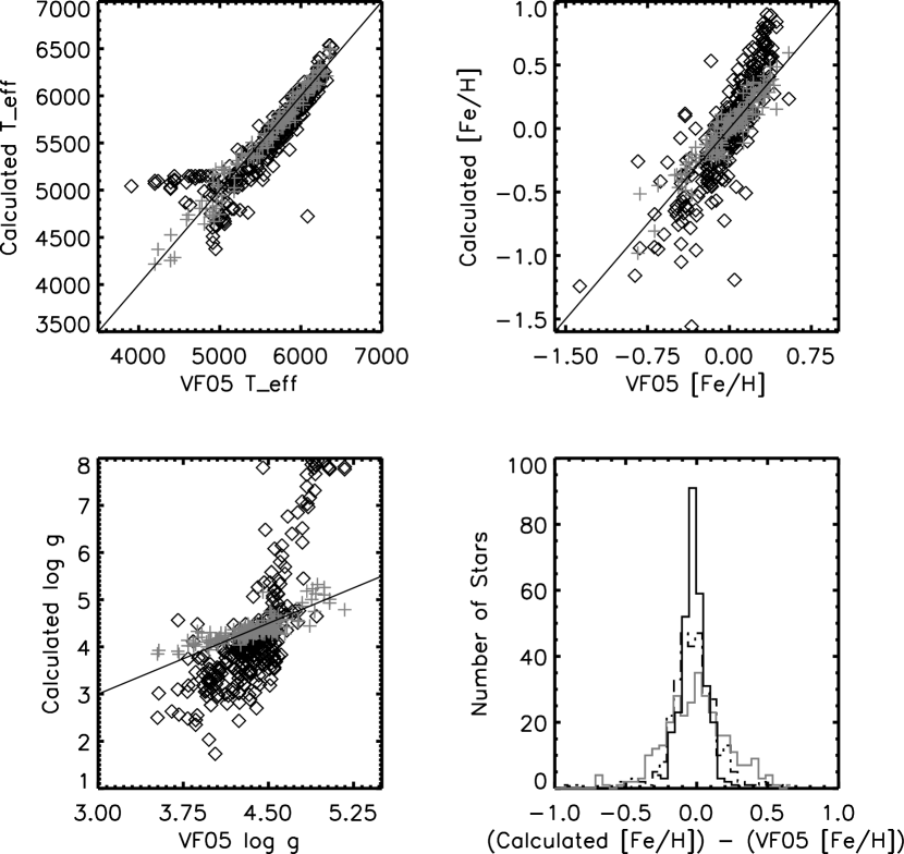
Figure 7: Results of inverting W94 fitting functions. Top left: $T_{\rm eff}$; top right: [Fe/H], bottom left: $\log\,g$. In each scatter plot, the black diamonds plot atmospheric-parameter values calculated using the WJ03 method against those of VF05. For comparison, the gray plus signs show the performance of the calibrations presented in this paper. The black, solid lines represent a 1:1 correlation. In the lower right, we show histograms of the residuals between metallicities determined by the WJ03 method and the VF05 values (solid gray); the WJ03-method residuals if the slope of the calculated vs. actual [Fe/H] trend is corrected to match the metallicity scale of VF05 (dotted black); and the residuals from our own calibration.

In Figure 7, we compare the results of the WJ03 method of finding atmospheric parameters with the new calibrations presented here. For stars warmer than 5015K, the two methods do a comparable job of finding effective temperature, though our calibrations show less scatter. For [Fe/H] and $\log\,g$, strong systematic differences are evident between the the two methods. The W94 metallicity scale appears to have a steeper tilt than that of VF05: Stars more metal-rich than the Sun have their metallicity substantially overpredicted by up to 0.5 dex, while [Fe/H] is underpredicted in stars more metal-poor than the Sun. In addition, as the histogram in Figure 7 shows, the [Fe/H] values found from the fitting functions are scattered more widely than those determined by our own calibrations. Since the systematic WJ03-method trend in [Fe/H] is mainly linear, the slope can be corrected to force the resulting [Fe/H] values to conform to the metallicity scale of VF05; doing so reduces $\sigma_{[Fe/H]}$ from 0.21 dex to 0.12 dex. The systematic trend in $\log\,g$ is even more pronounced, and has the added complication of being nonlinear: Fitting the WJ03-method results for stars with $\log\,g<4.5$ dex would yield a different slope than for stars with $\log\,g>4.5$ dex. Furthermore, there is substantial scatter in $\log\,g$ values found by inverting the W94 fitting functions for stars with $\log\,g<4.5$ dex.

Our $T_{\rm eff}$ calibration, $\sigma=82$K, performs comparably to that of Martell & Laughlin (2002), $\sigma=80$K. However, the benefits of using low-resolution spectroscopy are most evident when measuring [Fe/H] and $\log\,g$. Both of these parameters have only subtle effects on the shape of the stellar continuum, which can be measured well with photometry. Instead, [Fe/H] and $\log\,g$ change the depth and profile of broad spectral features in ways that are reflected in Lick indices. True empirical estimators for $\log\,g$ are uncommon in the literature; most methods are based on the combination of photometry and stellar models (see, e.g., Lastennet et al. 2001). One semiempirical calibration, based on photometry in the Vilnius system, is the Tautvaisiene & Lazauskaite (1993) GK-giants calibration ($0.5<\log\,g<3.0$ dex), which has precision $\sigma=0.3$ dex. Our $\log\,g$ calibration fills an important niche: It functions as a proof of concept for fully empirical modeling of $\log\,g$ (which is possible now that measurements from high-resolution spectra have become more precise and uniform), and it demonstrates the appreciable sensitivity of low-resolution spectra to $\log\,g$. Our [Fe/H] calibration, with $\sigma=0.07$ dex, is more precise than that of Martell & Laughlin (2002) ($\sigma_{\rm[Fe/H]}=0.10$ dex) or Schuster & Nissen (1989) ($\sigma_{\rm[Fe/H]}=0.13$ dex), and more accurate: Our Gaussian fit to the calibration residuals is centered at -0.017 dex, as opposed to -0.027 dex for Martell & Laughlin (2002) or -0.049 dex for Schuster & Nissen (1989).

4 $M_{V}$ and Distance Measurements

If one were to survey stars without Hipparcos parallaxes, as planet-search projects will certainly have to do within the next two years, it would be convenient to be able to estimate distances from low-resolution spectra. Such distance estimates could also be useful in screening photometric transit candidates emerging from projects such as the OGLE survey (Szymański 2005). The distance modulus can be calculated by interpolating stellar models to find the value of $M_{V}$ that matches a star’s effective temperature, surface gravity and metallicity. We used the Y² isochrones of Yi et al. (2001), for Solar abundance ratios and ages between 1 and 13 Gyr. The isochrones for the two metallicities surrounding the star’s [Fe/H] were interpolated in the $T_{\rm eff}$ and $\log\,g$ plane with a Gaussian-weighted sum of $M_{V}$ for the seven points nearest the star in temperature and gravity. We then interpolated the two resulting values of $M_{V}$ linearly in the metallicity dimension the to find the star’s absolute magnitude and distance modulus.

Figure 8 compares the absolute magnitude and distances estimated by our calibrations plus the Y² models with the Hipparcos values. This method gives distance measurements with uncertainty $0.2d$, where $d$ is the actual distance to the star—we are therefore estimating distance with $\sim 20\%$ accuracy. As expected, the limiting factor in our ability to spectroscopically estimate distance is the accuracy of the $\log\,g$ calibration: the $M_{V}$ scatter plot reflects the increased uncertainty in $\log\,g$ for subgiants and MSTO stars. The $M_{V}$ estimate also has a ceiling at 6.5 magnitudes beyond which it is no longer linear. This may reflect the sparseness of isochrone data points in $T_{\rm eff}$ and $\log\,g$ space for low-mass stars.

5 Planeticity Calibration

Martell & Laughlin (2002) suggested the possibility of finding an empirical calibration for “planeticity,” the presence or absence of a detectable planet around a star. Since the only known proxy for the presence of a planet is the metallicity, the best chance of creating a planeticity calibration should lie in finding trends in the abundance ratios of planet-bearing stars. One could then correlate Lick indices with other abundance ratios besides [Fe/H] and use these ratios to determine likely planeticity for each observed star. Even a minimally successful planeticity calibration would tremendously improve the observing efficiency of Doppler surveys.

Valenti & Fischer (2005) measured [Na/H], [Si/H], [Ti/H], [Fe/H] and [Ni/H], referenced to $\log\,N_{Fe}=7.50$, with other Solar abundances from Anders & Grevesse (1989). Planets have been found around 98 of 1040 stars. To form a calibration, we calculated each star’s metal-to-Hydrogen ratios as

$$M/H={N_{M}\over N_{H}}\,,$$

and each metal-to-metal ratio as

$$M_{1}/M_{2}={M_{1}/H\over M_{2}/H}\,.$$

We then used the Levenberg-Marquardt algorithm to find linear fits between the abundance ratios and several properties of the known extrasolar planets: $M\sin i$, $P$ and $M\sin i/P$ (a proxy for detectability, since high-mass and short-period planets are the easiest to detect). Stars without planets were assigned a planet mass of zero and a period of 5000 days. None of these fits were successful at replicating the properties of the training set. We also attempted a calibration aimed at discerning whether a particular star would have any planet at all, without reference to its mass or period: planet-bearing stars were assigned a planeticity of one, and stars without planets were assigned a planeticity of zero. As shown in Figure 9, this was unsuccessful: although stars with planets had slightly higher mean planeticity than those without, the calibration could not separate the populations of planet- and non-planet hosts.

One implication of the core accretion model of planet formation is that Oxygen-enhanced protostellar disks would have an enhanced probability of producing giant planets, which are thought to have cores composed mainly of H₂O ice. Therefore, if a chemical predictor of planeticity exists within the population of super-metal-rich stars, it is likely [$\alpha$/Fe]. With abundance data that included two Fe-peak elements (Fe and Ni) and two alpha elements (Si and Ti), we were unable to distinguish planet hosts from other stars. This might imply that alpha enhancement is not correlated with planet formation. It is also possible that a relationship between [$\alpha$/Fe] and planet formation exists, but we could not find it because our stars are of approximately Solar composition. Figure 10 shows [Si/Fe] vs. [Fe/H] for the Valenti & Fischer (2005) stars. [Si/Fe] in stars above Solar metallicity is confined to a tight locus that covers barely a factor of two. A more significant increase in alpha abundance may be necessary to increase the probability of planet formation. Finally, until terrestrial planets and planets at tens of AU from their host stars can be detected, we must assume that many stars that are presumed planetless do in fact have a system of satellites. This could preclude the possibility of a planeticity calibration, since these stars should not differ chemically from the stars that are known planet hosts. The dynamical interaction of the planets and the disk would likely determine the final configuration of the system.

6 Discussion

Our Lick-indices method of measuring atmospheric parameters has the advantage of being both precise and extremely efficient, requiring only one observation per star. Although small, systematic error trends no doubt remain in our calibrations, these systematics should match those contained in the VF05 dataset; our internal, random errors are small. The [Fe/H] and $T_{\rm eff}$ calibrations are especially robust and can be modestly extrapolated beyond the temperature and metallicity ranges of the training set. In producing our calibrations, we have been struck by the utility of linear or low-order fits involving several independent terms. These fits are more trustworthy than high-order fits on a few indices, which can be numerically unstable to interpolations even within the parameter space covered by the training-set data. We speculate that inverting the W94 fitting functions results in noticeable scatter of calculated atmospheric parameters because the fitting functions are third-order polynomials that may not be well behaved within the range of Lick indices analyzed here. Additionally, trial and error reveals that constructing a numerically robust empirical fit requires at least 10 times as many training-set members as terms in the calibration. Adding one or two thoughtfully chosen nonlinear terms, which can reasonably be expected to carry information about the parameter being measured, is therefore a far more economical way to make a fit more precise than increasing the order of the fit, which would necessitate the addition of many new training-set members (in this case, observations).

With our $T_{\rm eff}$ calibration, we are able to screen out candidate stars hotter than the $\sim{\rm F}7$ temperature limit for combined high-accuracy spectral synthesis modeling and $3-5\>{\rm ms^{-1}}$ Doppler precision (Fischer & Valenti 2005). Our $\log\,g$ calibration is currently valid for FGK main-sequence dwarfs because these stars comprise the bulk of the VF05 training set used to build the calibrations.

Certainly, as Doppler velocity surveys are extended to include stars that lack accurate Hipparcos parallaxes, it will be vital to extend the $\log\,g$ calibration to subgiants and giants. This extension should be straightforward given an adequate training set, and would be of considerable value. It could also be used, for example, to select stars in the Hertzsprung gap for inclusion in radial-velocity surveys (see Sato et al. 2005b, Johnson 2005). Stars that are evolving across the Hertzsprung gap are intrinsically luminous and relatively rare, and hence tend to lie outside the regime of good trigonometric parallaxes. Characterization of such stars is, however, a matter of great current interest for radial-velocity programs because many members of this population were originally early F through late B stars when they were on the main sequence. By monitoring Hertzsprung gap stars with the Doppler technique, one can probe the planetary distribution endemic to stars in the range $1.5M_{\odot}$ to $5M_{\odot}$. In any event, our current $T_{\rm eff}$ and $\log\,g$ calibrations can be combined with the $Y^{2}$ stellar models to give $20\%$-accurate distance estimates for nearby stars.

A planeticity calibration tied to specific abundance ratios remains a tantalizing idea, but we find that [Fe/H] remains the best predictor of presence of a detectable planet. By screening stars for high [Fe/H] with our Lick indices calibration, we can use the planet-metallicity correlation to increase the efficiency of Doppler planet searches. The N2K Consortium is obtaining low-resolution spectra of 2000 high-metallicity candidate stars (Robinson et al. 2005, in preparation), from which we expect to identify $\sim 500$ stars with ${\rm[Fe/H]}\geq 0.2\,{\rm dex}$. This pool should yield $\sim 30$ hot Jupiters and 2-3 transits of stars bright enough for high-precision follow-up studies from both ground and space.

Figure 1: Unsharp masking method. A smoothed version of each spectrum is subtracted from the original spectrum. Line centers are then located in the unsharp-masked spectrum by searching for minima in a $20\>\AA$ window around where each line should fall. This spectrum of HD 117176 was taken with the Nickel spectrograph.

Figure 2: Comparison between observed equivalent widths (y-axis) and those published in Worthey et al. (1994) (x-axis) for the 12 indices used in our fits to stellar atmospheric parameters. Strongly deviant points in metal-line measurements correspond to metal-poor stars ([Fe/H] $\leq-1.5$ dex); deviant points in Balmer-line measurements correspond to cool stars (spectral type K4 or later). These points were not used to transform our data to the Lick/IDS system.

Figure 3: Left: Scatter plot showing the performance of the $T_{\rm eff}$ calibration. The solid line shows a theoretical perfect fit, and the dotted lines show the calibration’s 1-$\sigma$ error. Right: Histogram of the residuals of the $T_{\rm eff}$ calibration. The residuals are well modeled by a Gaussian distribution with $\sigma=82$K, centered at -28.4K.

Figure 4: Left: Scatter plot showing the performance of the [Fe/H] calibration. The solid line shows a theoretical perfect fit, and the dotted lines show the calibration’s 1-$\sigma$ error. Right: Histogram of the residuals of the [Fe/H] calibration. The residuals are well modeled by a Gaussian distribution with $\sigma=0.07$ dex, centered at -0.017 dex.

Figure 5: Left: Scatter plot showing performance of $\log\,g$ calibration. The solid line shows a theoretical perfect fit, and the dotted lines show the calibration’s 1-$\sigma$ error. Although stars with $\log\,g\geq 3.5$ formed the training set, this calibration is not effective at separating subgiants and dwarfs; thus we report its useful range as $4.0<\log\,g<5.1$. Right: Histogram of the residuals of the $\log\,g$ calibration. The residuals are well modeled by a Gaussian distribution with $\sigma=0.13$ dex, centered at -0.038 dex.

Figure 6: Modified HR diagram of the VF05 stars in our dataset. Instead of luminosity, we have plotted $\log\,g$ on the vertical axis, showing that the divide between dwarfs and subgiants occurs at $\log\,g\sim 4.0$ dex.

Figure 8: Left: Comparison of M_V estimates from our calibrations and Y² isochrones to Hipparcos values. Right: Comparison of estimated distances and Hipparcos values. In both plots, the solid line represents a 1:1 correlation.

Figure 9: Histograms of calculated planeticity for non-planet-bearing stars (dashed line) and planet-bearing stars (solid line). Stars without planets were assigned a planeticity of 0, and stars with planets were assigned a planeticity of 1. The calibration is not able to distinguish stars with planets based on metal abundances.

Figure 10: [Si/Fe] vs. [Fe/H] for the stars in the VF05 data set. None of the metal-rich stars show significant alpha enhancement.

Table 1: Matching the Lick system: Linear transformations from observed to published Lick indices and index errors

Index	Slope	Intercept	Error	N Rejected
Ca4227	1.170	-0.081	0.216	2
	1.101	-0.309	0.210	1
G4300	1.182	-0.854	0.439	2
	1.229	-0.911	0.372	3
HgF	1.079	-0.250	0.387	2
	1.068	-0.019	0.520	3
Fe4383	1.016	0.287	0.569	1
	0.975	-0.575	0.693	1
Fe4531	1.011	-0.182	0.316	1
	0.988	-0.401	0.402	1
Fe4668	1.092	-0.526	0.588	2
	1.067	-0.234	0.607	2
Hbeta	1.021	-0.200	0.236	2
	0.991	-0.133	0.161	2
Fe5015	1.198	0.066	0.580	0
	1.055	-0.278	0.501	0
Mg2	1.043	0.044	0.009	1
	1.036	0.033	0.010	1
Mgb5177	1.490	0.590	0.298	1
	1.376	0.518	0.355	2
Fe5270	1.203	-0.021	0.234	1
	1.186	-0.257	0.308	0
Fe5406	1.348	-0.215	0.247	1
	1.183	-0.313	0.223	2
Na5895	1.004	0.219	0.303	1
	1.149	-0.279	0.211	2

Table 2: Lick Indices for Training-Set Stars.

HD	Site	Ca4227	G4300	H$\gamma_{F}$	Fe4383	Fe4531	Fe4668	H$\beta$	Fe5015	Mg2	Mg $b$	Fe5270	Fe5406	Na D
400	N	0.482	1.13	2.13	0.975	1.88	1.24	3.42	3.37	0.0696	1.29	1.34	0.352	1.04
	N	0.482	1.13	2.13	0.975	1.88	1.24	3.42	3.37	0.0696	1.29	1.34	0.352	1.04
691	N	0.977	5.51	-1.69	4.63	3.01	4.98	2.19	6.09	0.198	3.95	3.43	2.09	2.26
	N	0.977	5.51	-1.69	4.63	3.01	4.98	2.19	6.09	0.198	3.95	3.43	2.09	2.26
3079	N	0.477	2.84	1.54	1.61	1.99	1.77	3.05	4.15	0.0828	1.66	1.68	0.716	1.08
	N	0.477	2.84	1.54	1.61	1.99	1.77	3.05	4.15	0.0828	1.66	1.68	0.716	1.08
	K	0.470	3.59	1.05	2.79	2.30	1.58	3.15	3.46	0.0807	1.52	1.35	0.516	0.861
3765	K	2.99	5.83	-1.58	8.63	4.36	6.27	1.06	6.33	0.386	6.86	4.19	2.82	4.70
3770	K	0.410	4.22	1.18	2.58	2.36	1.79	3.16	3.68	0.0759	0.905	1.26	0.493	1.16
4256	K	3.81	5.71	-1.77	8.23	4.84	7.36	1.80	6.49	0.458	8.02	4.33	3.25	6.20
	K	3.73	5.96	-1.91	9.61	4.86	7.17	0.857	6.53	0.459	8.11	4.36	3.26	6.23
4903	K	0.305	3.75	1.25	2.50	2.44	1.84	3.30	3.52	0.0763	1.27	1.30	0.534	0.959
5470	K	0.625	4.81	0.268	3.85	2.88	4.26	3.13	4.81	0.117	2.13	1.99	0.848	1.62
6963	K	1.28	5.03	-1.83	4.91	2.84	2.73	2.00	4.13	0.157	3.40	2.31	1.33	1.75
7590	K	0.694	3.87	0.531	2.90	2.43	1.90	2.82	3.71	0.0946	1.96	1.52	0.704	1.12
8331	K	0.640	5.73	-1.12	4.09	2.76	3.43	2.44	4.34	0.117	1.96	1.90	0.923	1.31
9070	K	1.11	5.20	-1.21	5.51	3.28	5.75	2.73	5.65	0.170	3.04	3.07	1.41	2.39
9331	K	1.20	5.59	-1.50	5.58	3.31	5.20	2.56	5.36	0.169	3.37	2.69	1.35	1.98
10086	K	1.07	4.66	-1.17	4.67	2.99	4.11	2.47	4.78	0.147	2.78	2.27	1.22	1.68
11850	K	1.26	5.12	-1.47	4.85	3.01	3.74	2.19	4.67	0.152	2.97	2.43	1.25	1.73
	K	1.20	5.26	-1.29	4.89	3.04	3.86	2.36	4.65	0.155	2.95	2.56	1.30	1.89
12235	K	0.512	4.67	0.515	3.51	2.90	4.33	3.24	4.74	0.111	1.82	2.03	0.743	1.61
12328	K	1.62	5.85	-1.69	6.87	3.72	6.11	1.30	5.60	0.248	4.82	3.55	2.17	2.70
12414	K	0.227	2.42	2.72	0.902	1.69	0.809	3.63	2.24	0.0554	0.980	0.972	0.276	0.899
12661	K	0.662	5.36	-1.33	5.29	3.22	6.80	2.73	5.67	0.180	3.34	2.64	1.34	2.31
12846	K	0.824	5.15	-1.15	3.83	2.35	2.32	2.28	3.59	0.129	2.70	1.71	0.798	1.38
13531	K	1.19	5.18	-1.45	4.50	3.03	3.38	2.09	4.53	0.150	2.83	2.31	1.25	1.77
13825	K	0.708	5.37	-1.39	5.00	3.17	5.29	2.58	5.10	0.174	2.96	2.40	1.17	2.08
16275	K	0.826	4.67	-0.482	4.72	3.14	5.43	2.87	5.34	0.140	2.96	2.61	1.18	2.18
17230	K	6.86	5.55	-1.58	8.34	5.40	-3.20	1.45	6.32	0.572	8.53	5.28	4.14	11.3
	K	6.78	5.48	-1.44	8.09	5.57	-3.07	1.27	6.32	0.569	8.38	5.27	4.19	11.3
18143	K	2.35	5.55	-1.69	8.17	4.11	7.39	1.45	6.40	0.344	5.76	3.74	2.48	4.41
18803	K	0.911	4.90	-1.15	3.74	3.01	4.57	2.47	4.51	0.170	3.71	2.90	1.24	2.27
19373	K	0.587	4.26	0.727	2.30	2.62	2.96	3.09	4.28	0.104	2.01	1.90	0.755	1.55
21019	K	0.526	5.63	-1.71	3.61	2.36	2.03	1.73	3.48	0.105	1.83	1.54	0.765	1.38
21197	K	5.97	5.45	-1.59	8.79	5.65	-2.00	1.68	6.91	0.556	9.12	5.58	4.15	10.5
22072	K	1.06	6.07	-1.99	4.57	3.09	4.29	1.28	4.65	0.207	3.87	2.53	1.47	1.84
23249	K	1.19	6.14	-1.66	6.96	3.69	7.76	1.51	5.77	0.257	3.98	3.50	2.14	3.25
23596	K	0.542	4.63	0.527	3.56	2.93	3.97	3.34	4.73	0.110	1.62	1.83	0.794	1.53
	K	0.529	4.61	0.476	3.96	2.96	3.72	3.31	4.74	0.109	1.51	2.03	0.746	1.57
	K	0.575	4.66	0.529	3.53	2.66	3.73	3.26	4.70	0.106	1.83	2.01	0.863	1.74
24365	K	0.809	6.37	-2.91	5.17	3.04	4.01	1.57	4.23	0.152	2.36	2.47	1.17	1.69
24916	K	5.88	5.32	-1.26	8.41	5.39	-2.16	1.67	5.56	0.498	8.16	5.34	3.75	7.46
25069	K	0.954	6.10	-1.87	6.53	3.84	7.22	1.48	5.89	0.239	4.00	3.68	2.29	3.00
25790	K	0.611	5.47	-1.46	4.54	3.06	4.89	2.21	4.62	0.129	2.27	2.32	1.16	1.88
26794	K	3.67	5.51	-1.61	8.15	4.17	5.56	0.705	5.85	0.443	8.84	4.29	2.87	5.42
28005	K	0.477	5.12	-0.714	4.47	3.16	5.84	2.87	5.54	0.156	2.71	2.28	1.14	2.17
30508	K	0.838	6.38	-2.58	5.33	3.14	4.87	1.64	4.45	0.159	2.54	2.54	1.40	1.98
30825	K	0.825	6.28	-1.62	4.71	3.14	3.85	1.44	4.64	0.158	2.53	2.39	1.40	1.72
34575	K	0.955	5.32	-1.93	5.80	3.41	6.55	2.39	5.39	0.192	3.20	3.04	1.53	2.59
52456	N	2.34	6.64	-1.78	7.05	3.25	5.07	1.41	5.74	0.282	5.35	3.56	2.38	3.41
52711	N	1.03	4.44	0.374	2.99	2.54	2.20	2.69	3.83	0.110	2.37	1.75	0.745	1.37
56124	N	1.05	4.58	-0.0229	3.65	2.58	2.58	2.75	3.89	0.121	2.41	1.96	0.991	1.50
56303	N	0.982	4.36	0.697	3.43	2.49	3.44	3.07	4.34	0.111	2.15	2.10	0.840	1.44
58781	N	1.24	5.67	-1.45	4.81	3.05	4.75	2.38	4.87	0.177	3.04	2.72	1.17	2.21
59747	N	2.84	7.34	-2.06	7.03	3.79	-0.526	1.29	3.92	0.299	5.93	4.01	2.60	3.24
63433	N	1.39	5.13	-0.598	4.44	2.73	3.24	2.27	4.58	0.143	2.78	2.47	1.28	1.69
64468	N	3.44	6.84	-2.10	8.73	4.14	0.925	1.03	5.95	0.447	7.87	4.80	2.89	5.02
65430	N	2.07	6.84	-2.17	5.92	3.24	4.96	1.57	5.21	0.303	6.46	3.19	1.73	3.09
65583	N	1.70	5.67	-1.97	4.04	2.18	0.0508	1.58	3.46	0.206	4.96	2.03	0.797	1.91
67767	N	0.909	6.12	-2.03	5.05	2.80	4.44	1.82	5.02	0.163	3.06	2.50	1.40	1.84
68017	N	1.12	5.35	-1.14	3.71	2.04	2.21	2.07	3.30	0.154	3.43	1.71	0.599	1.52
69809	N	1.06	5.24	-0.265	4.25	2.79	5.65	2.96	5.27	0.150	2.87	2.52	1.04	1.98
70843	N	0.612	3.35	2.33	2.20	2.20	2.58	3.80	4.21	0.0856	1.34	1.80	0.661	1.39
72780	N	0.683	2.70	2.42	2.33	2.17	1.81	3.62	4.21	0.0844	1.32	1.86	0.621	1.26
73344	N	0.723	3.66	1.58	2.52	2.36	2.57	3.35	3.87	0.0925	1.78	1.72	0.653	1.25
73667	N	2.77	6.39	-1.83	5.73	2.98	1.99	0.981	4.45	0.343	7.34	2.91	1.90	3.04
73668	N	0.929	4.11	0.684	3.04	2.50	2.44	3.02	3.95	0.107	2.01	1.98	0.931	1.67
74156	N	0.729	4.00	1.07	2.53	2.31	3.01	3.30	4.48	0.0997	1.98	1.92	0.974	1.64
75302	N	1.07	5.04	-0.748	4.46	2.80	3.60	2.56	4.70	0.148	2.64	2.63	1.43	1.89
75332	N	0.540	2.92	2.01	2.27	2.11	1.52	3.60	4.39	0.0895	1.75	1.80	0.678	1.35
75732	N	1.06	6.57	-1.43	6.91	3.47	8.94	1.83	6.65	0.308	5.37	3.80	2.29	3.90
75782	N	0.323	4.60	0.802	2.90	2.87	3.73	3.22	5.03	0.104	1.56	2.06	0.845	1.37
76909	N	0.188	5.21	-0.941	4.11	3.01	7.30	2.85	6.25	0.184	3.71	2.74	1.33	2.42
80367	N	2.60	6.47	-1.68	7.20	3.70	5.66	1.20	5.51	0.349	7.77	3.86	2.56	3.39
80606	N	1.03	5.79	-1.43	6.15	3.08	7.56	2.45	4.04	0.225	3.94	3.22	1.73	2.81
82106	N	4.29	6.79	-1.67	9.06	4.70	-0.726	1.50	3.60	0.428	8.25	4.70	3.32	4.81
87836	N	0.794	5.80	-0.709	4.00	3.07	6.72	2.77	5.67	0.164	2.73	2.69	1.42	1.87
87883	N	3.11	6.55	-1.53	8.55	3.90	5.62	0.882	6.23	0.408	7.96	4.64	2.94	4.62
88371	N	1.05	5.19	-0.426	3.14	2.94	2.99	2.43	3.82	0.152	3.23	1.86	0.826	1.35
88986	N	0.819	5.21	-0.108	3.06	2.87	3.53	2.58	4.37	0.117	2.39	1.84	0.931	1.37
89269	N	1.07	5.33	-0.959	4.11	2.61	2.76	1.88	3.96	0.142	3.09	2.12	0.987	1.52
89307	N	0.744	4.03	0.694	2.51	2.29	2.15	2.95	3.73	0.103	2.19	1.69	0.825	1.18
91204	N	0.697	4.94	0.235	3.42	2.63	4.34	2.94	4.79	0.127	2.62	2.32	1.13	1.74
95128	N	0.831	4.89	0.318	3.09	2.66	3.05	2.62	3.76	0.110	2.40	1.74	0.771	1.08
96418	N	0.453	2.85	2.62	1.25	2.31	1.33	3.56	3.86	0.0729	1.11	1.51	0.548	0.911
96574	N	0.774	3.66	1.78	1.95	2.27	2.15	3.41	3.78	0.0866	1.66	1.59	0.890	1.02
97004	N	0.743	5.42	-1.22	5.52	3.61	7.57	2.46	5.84	0.214	4.39	3.18	1.47	2.45
98388	N	0.449	2.06	2.87	1.77	2.17	1.49	3.80	3.89	0.0786	1.38	1.54	0.505	0.899
98697	N	0.398	3.29	1.87	1.44	2.08	1.67	3.33	3.44	0.0741	1.09	1.51	0.434	1.06
99491	N	1.25	5.94	-2.08	5.60	3.20	7.69	2.11	5.93	0.231	4.67	3.30	1.65	2.78
99492	N	3.59	6.78	-1.87	9.51	4.76	7.58	0.730	6.63	0.461	8.87	4.81	3.59	5.95
100180	N	0.576	4.01	0.865	2.65	2.42	2.20	2.89	3.92	0.0957	1.97	1.62	0.654	1.13
102158	N	0.777	4.94	-0.299	2.87	2.11	1.20	2.16	2.46	0.111	2.52	1.37	0.423	0.999
103095	N	1.91	5.05	-0.409	3.44	1.69	-0.143	0.998	1.22	0.179	4.34	1.71	0.614	1.12
103432	N	0.835	5.05	-1.10	4.09	3.08	3.05	2.24	4.52	0.145	3.38	2.74	1.30	1.64
104556	N	1.24	6.78	-2.49	4.33	3.06	3.50	1.01	4.28	0.197	4.30	2.32	1.24	1.47
104800	N	0.944	4.63	0.261	2.01	2.09	0.536	2.42	2.42	0.108	2.50	1.05	-0.0899	0.922
105405	N	0.574	3.08	2.01	1.49	1.96	1.10	3.35	3.44	0.0761	1.47	1.27	0.580	1.03
105631	N	1.43	5.88	-1.95	6.31	3.65	6.01	1.89	5.74	0.227	4.36	3.58	2.11	2.59
106156	N	1.66	6.54	-2.26	6.46	3.54	6.53	1.91	5.43	0.238	4.71	3.56	1.86	2.66
106252	N	0.822	4.81	0.0376	2.92	2.67	2.63	2.70	3.98	0.109	2.09	1.69	0.913	1.17
106423	N	0.737	4.47	0.680	3.34	2.87	4.89	3.30	5.63	0.120	2.13	2.47	1.03	1.53
107146	N	1.08	4.77	0.0711	3.36	2.93	2.96	2.52	4.14	0.118	2.19	1.86	1.11	1.23
107213	N	0.476	3.29	2.03	1.41	2.60	2.98	3.63	4.31	0.0711	1.39	1.55	0.481	0.914
107705	N	0.830	3.18	1.72	2.43	2.53	2.53	3.18	3.80	0.0805	1.44	1.65	0.590	0.979
108874	N	0.898	5.74	-1.78	5.26	2.76	6.30	2.31	5.42	0.193	3.83	2.96	1.52	2.24
109358	N	0.713	4.49	0.102	2.20	2.21	1.97	2.64	3.47	0.0971	1.95	1.43	0.665	1.06
110315	N	5.66	6.75	-2.06	8.58	5.22	2.51	1.34	6.08	0.608	10.5	4.92	3.63	7.07
111066	N	0.597	3.62	1.47	2.05	2.07	1.93	3.40	3.83	0.0797	1.55	1.54	0.603	0.955
111395	N	1.47	5.32	-1.04	4.63	2.98	4.07	2.01	4.26	0.141	3.00	2.28	1.09	1.56
111398	N	0.944	5.81	-0.720	3.64	2.83	4.18	2.51	4.89	0.146	2.66	2.42	1.16	1.50
111515	N	1.22	5.93	-1.41	3.38	2.58	1.23	1.60	3.33	0.177	4.10	2.04	0.746	1.59
112060	N	0.814	6.44	-2.00	4.91	3.21	6.26	1.86	4.91	0.146	2.54	2.44	1.10	1.49
114174	N	0.900	5.22	-0.598	3.64	2.82	3.52	2.34	4.44	0.142	2.75	2.30	1.17	1.59
114762	N	0.493	3.95	0.905	1.93	1.80	0.339	2.54	2.41	0.0811	1.77	1.07	0.239	0.988
116442	N	1.64	6.32	-1.67	5.07	3.17	2.09	1.15	3.23	0.241	5.74	2.69	1.79	2.38
116443	N	2.14	5.99	-1.79	6.38	3.26	2.53	0.885	4.38	0.314	6.88	3.23	1.90	2.78
117126	N	0.924	5.27	-0.629	3.75	2.81	3.65	2.35	4.03	0.133	2.32	2.12	0.977	1.42
117176	N	0.968	5.89	-1.26	3.62	2.73	3.40	1.85	3.74	0.111	2.38	1.70	0.708	1.00
117936	N	3.85	6.30	-1.26	9.57	5.22	-0.730	1.51	5.11	0.471	8.22	4.74	3.38	5.85
118914	N	0.816	4.84	-0.211	3.72	2.77	0.454	2.71	4.14	0.152	2.25	2.56	1.19	1.55
120066	N	0.873	4.54	0.517	2.88	2.91	2.81	2.56	4.37	0.101	2.13	1.71	0.724	1.00
120136	N	0.654	2.38	3.07	1.78	2.65	1.72	4.12	4.19	0.0760	1.21	1.50	0.429	1.07
121560	N	0.453	3.26	1.72	1.44	1.71	0.118	3.13	2.56	0.0749	1.49	0.875	0.592	0.932
122120	N	4.84	4.39	-1.02	9.02	5.26	-1.91	0.317	6.62	0.563	8.89	4.92	3.82	8.01
122652	N	0.465	2.70	1.81	2.41	2.25	1.54	3.52	2.56	0.0894	1.83	1.64	0.649	1.10
122676	N	1.14	5.60	-1.37	4.33	2.96	3.82	2.20	4.63	0.174	3.55	2.31	1.65	2.30
124642	N	4.88	6.09	-1.15	9.67	4.99	-1.25	1.37	5.17	0.472	7.78	5.05	3.51	5.90
124694	N	0.474	3.28	1.68	1.95	2.10	2.17	3.37	3.79	0.0836	1.72	1.66	0.544	0.992
125040	N	0.652	1.91	2.54	1.71	2.03	0.927	3.71	3.37	0.0900	1.42	1.70	0.767	1.13
126053	N	1.08	5.29	-0.550	3.06	1.90	-0.757	2.15	2.27	0.123	2.61	1.56	0.480	1.25
126961	N	0.780	3.23	1.98	2.32	1.99	2.16	3.48	4.24	0.0892	1.60	1.60	0.801	1.22
127334	N	0.793	5.56	-1.11	4.31	2.71	5.91	2.36	5.25	0.148	2.88	2.25	1.15	1.60
128165	N	3.86	6.42	-1.39	8.34	4.28	-1.51	0.730	4.94	0.458	8.34	4.41	3.22	5.21
130087	N	0.692	4.68	0.773	2.79	2.59	4.04	3.02	5.97	0.119	1.96	2.14	0.919	1.66
130307	N	2.97	6.79	-1.34	6.87	3.71	-1.20	1.10	3.46	0.330	7.00	3.61	2.08	3.37
130322	N	1.71	6.98	-1.38	6.39	3.34	4.76	1.77	3.73	0.219	4.48	3.13	1.88	2.45
130871	N	3.21	6.64	-1.02	7.29	3.00	-1.29	0.666	3.59	0.441	8.67	4.27	2.60	4.47
131509	N	1.29	7.36	-1.75	5.58	2.99	5.37	1.43	3.12	0.217	4.12	3.12	1.77	2.16
132142	N	1.90	6.02	-2.49	5.64	2.91	3.58	1.27	4.19	0.287	6.24	3.03	1.63	2.39
133161	N	0.730	4.30	0.888	2.94	2.54	3.83	3.27	4.77	0.116	2.31	2.11	0.863	1.48
	K	0.595	4.34	0.800	2.92	2.84	3.56	3.33	4.68	0.104	1.69	1.86	0.820	1.69
133460	N	0.810	4.22	1.46	2.75	2.43	2.55	3.42	5.10	0.103	1.84	1.79	0.973	1.36
134044	N	0.589	3.20	1.94	1.93	2.12	2.27	3.56	4.31	0.0841	1.47	1.71	0.590	1.00
135101	N	0.799	5.52	-0.952	3.79	2.60	4.92	2.27	4.78	0.150	2.96	1.94	0.901	1.29
135599	N	2.22	6.71	-1.71	6.07	3.23	-0.668	1.51	3.88	0.254	5.15	3.15	1.81	2.38
136118	K	0.438	3.62	1.65	2.13	2.21	1.50	3.38	3.30	0.0633	0.883	1.25	0.401	1.15
136442	K	2.25	6.24	-2.15	8.44	4.43	9.95	1.16	7.13	0.363	6.83	4.55	2.93	4.44
136544	N	0.610	0.327	4.47	1.51	2.19	1.54	4.15	4.24	0.0787	1.46	1.65	0.541	0.994
	K	0.356	2.61	3.29	0.954	2.36	1.51	4.15	3.96	0.0628	1.11	1.38	0.395	1.22
136580	N	0.271	2.57	2.11	1.67	1.74	1.07	3.48	3.54	0.0750	1.48	1.25	0.443	0.947
136654	N	0.538	2.70	2.54	1.39	2.13	1.96	3.97	4.14	0.0726	1.17	1.44	0.537	1.02
136834	N	3.27	6.93	-1.62	10.1	3.67	7.58	1.04	4.70	0.456	8.49	4.53	3.24	5.70
136923	N	1.87	6.52	-1.67	5.59	3.20	4.00	1.76	3.45	0.219	4.54	2.70	1.64	2.16
137510	N	0.113	2.90	2.53	3.35	2.52	4.37	3.37	5.73	0.125	2.30	2.15	0.994	1.43
	K	0.435	4.84	0.604	3.04	3.13	4.69	3.25	5.29	0.108	1.62	1.99	0.855	1.62
137778	K	2.44	5.86	-1.55	8.10	4.21	6.46	1.43	6.59	0.315	5.48	3.93	2.63	4.67
138573	N	0.847	5.39	-0.569	4.23	2.37	3.43	2.44	3.05	0.142	2.56	2.25	1.07	1.56
139323	N	3.20	6.50	-3.09	8.44	4.57	8.86	1.29	8.03	0.395	6.65	4.64	3.15	4.72
139324	N	0.755	5.02	0.240	2.99	2.55	3.57	2.89	5.18	0.116	1.96	2.08	1.01	1.45
	K	0.520	4.80	-0.0381	3.86	2.60	3.43	2.98	4.55	0.113	1.93	1.88	0.781	1.55
139457	N	0.429	3.02	1.71	1.70	1.84	0.496	2.97	1.52	0.0706	1.36	1.21	0.523	1.05
	K	0.320	3.49	1.68	1.34	1.78	0.464	3.15	2.54	0.0648	1.02	1.13	0.242	0.922
142229	N	0.951	4.46	0.391	3.33	2.04	-1.09	2.53	4.57	0.120	2.21	2.34	1.11	1.67
	N	0.731	3.89	0.787	2.27	2.31	2.01	2.74	4.60	0.109	2.53	2.32	0.962	1.61
	K	0.807	4.39	0.0796	3.58	2.68	2.67	2.71	4.24	0.105	1.96	1.78	0.888	1.55
142373	N	0.154	4.51	0.520	1.84	1.84	0.574	2.28	3.11	0.0841	1.52	1.45	0.467	1.06
143291	N	1.66	6.33	-1.58	5.31	2.63	-0.778	1.59	4.12	0.227	4.80	2.49	1.42	1.94
	N	1.46	6.08	-1.20	4.43	2.43	2.93	1.26	4.06	0.226	5.64	2.61	1.52	2.03
143761	N	0.794	4.66	0.0369	2.62	2.14	1.82	2.41	3.74	0.108	2.27	1.38	0.399	1.05
	K	0.660	4.76	-0.191	3.09	2.25	1.79	2.44	3.59	0.101	2.11	1.37	0.637	1.19
144579	N	1.58	5.76	-2.31	3.97	2.05	1.86	1.38	2.20	0.208	5.12	1.77	0.893	1.69
145229	N	0.652	3.96	0.453	2.64	2.66	1.48	2.58	3.98	0.104	2.09	1.62	0.624	1.33
148467	N	6.14	4.73	-1.52	8.05	5.68	-2.99	1.79	4.73	0.581	9.23	5.04	4.04	8.80
	K	6.91	5.55	-1.35	8.63	5.56	-3.24	1.33	5.90	0.559	8.38	5.00	3.91	9.80
149200	K	0.600	2.90	2.35	2.32	2.40	2.07	3.73	4.00	0.0665	1.37	1.38	0.521	1.04
149652	N	0.435	2.84	2.35	1.57	1.77	0.811	3.60	2.95	0.0745	0.941	1.48	0.490	0.964
149661	N	1.43	6.35	-1.01	5.66	3.35	4.51	1.42	5.62	0.270	5.39	3.31	2.05	2.95
149806	N	1.60	6.74	-1.64	6.86	3.34	6.78	1.76	4.03	0.270	5.42	3.32	2.10	3.04
150933	N	0.841	3.88	1.33	2.60	2.37	2.46	3.29	4.49	0.104	1.67	1.64	0.721	1.30
151044	N	0.709	3.75	1.64	2.16	2.02	1.72	3.15	3.86	0.0922	1.47	1.59	0.708	1.01
151090	N	1.40	7.60	-1.85	5.66	2.76	4.18	1.22	4.67	0.200	3.82	2.36	1.28	1.51
	K	1.25	6.02	-1.86	5.27	3.21	4.44	1.31	4.70	0.203	3.74	2.62	1.51	1.93
	K	1.22	6.16	-1.62	5.21	3.19	4.76	1.30	4.40	0.202	3.90	2.74	1.51	2.01
151288	N	7.44	5.26	-1.32	8.42	5.26	-2.21	1.25	6.50	0.552	7.86	5.07	4.29	10.8
151877	N	2.31	6.98	-1.78	5.78	2.84	4.28	1.61	5.78	0.264	5.39	3.29	1.70	2.73
	K	1.96	5.58	-1.54	6.58	3.39	3.90	1.46	5.11	0.250	5.34	3.36	1.97	3.06
152446	N	0.575	2.68	1.96	1.80	1.80	1.49	3.40	3.68	0.0746	1.17	1.19	0.355	0.936
	N	0.508	2.77	1.96	1.12	1.79	0.800	3.30	3.71	0.0851	1.15	1.37	0.445	1.02
152792	K	0.500	5.06	-0.609	3.29	2.19	1.54	2.21	3.38	0.0910	1.77	1.48	0.587	1.17
153627	N	0.612	4.29	0.859	2.63	1.75	0.733	2.91	3.66	0.0985	1.56	1.59	0.496	0.975
154160	N	0.861	5.62	-1.48	4.78	3.02	7.60	2.49	3.82	0.166	2.69	2.49	1.24	1.77
	N	0.546	5.75	-1.16	4.20	2.76	7.51	2.48	6.46	0.189	3.35	2.92	1.53	2.14
154345	N	1.25	5.50	-1.56	4.24	2.64	3.24	1.93	4.84	0.196	3.97	2.48	1.43	2.04
154363	K	6.56	5.56	-1.72	7.37	4.63	-2.61	1.09	5.84	0.592	9.59	4.50	3.19	8.28
	K	6.34	5.12	-1.56	7.34	4.60	-2.32	1.04	5.79	0.600	9.84	4.44	3.12	8.25
154417	N	0.850	3.90	1.02	2.98	2.27	1.73	3.12	4.67	0.101	1.87	1.92	0.844	1.08
155060	N	0.843	3.99	1.01	2.18	2.07	1.37	2.98	2.76	0.0942	1.67	1.55	0.637	1.06
155423	N	0.666	3.37	1.97	2.38	2.23	2.92	3.66	5.10	0.0988	1.53	1.76	0.503	1.17
156826	K	0.889	6.10	-1.82	5.24	3.04	3.78	1.41	4.41	0.157	3.30	2.61	1.35	2.06
157214	N	1.06	5.19	-0.397	2.93	2.14	2.31	2.35	3.95	0.126	2.80	1.42	0.555	1.08
157466	N	0.569	3.14	1.54	1.63	1.58	0.757	2.94	1.87	0.0795	1.41	0.897	0.384	0.923
157881	N	6.62	4.62	-1.48	7.86	5.57	-3.13	1.13	5.54	0.545	7.68	5.01	3.80	10.7
	K	6.36	4.86	-1.20	7.67	5.50	-3.11	1.30	5.79	0.529	7.18	5.14	4.00	12.3
	K	6.33	4.73	-1.15	7.05	5.53	-3.08	1.28	5.81	0.526	7.15	5.24	4.03	12.5
159063	N	0.642	3.14	2.39	2.04	2.28	2.43	3.85	4.98	0.0943	1.48	1.63	0.660	1.15
159222	N	0.952	4.78	0.0173	4.02	2.33	3.39	2.76	4.77	0.123	2.04	1.95	0.816	1.38
159909	N	1.11	5.46	-0.780	3.87	2.80	4.73	2.65	5.26	0.155	2.85	2.16	1.09	1.64
160693	N	0.720	5.07	-0.0442	2.57	1.71	1.08	2.50	3.80	0.106	1.92	1.05	0.316	0.899
161797	N	1.03	5.20	-1.12	4.49	2.90	7.12	2.48	5.98	0.174	2.77	2.75	1.49	1.90
161848	N	2.42	6.78	-1.76	5.88	3.10	2.47	1.27	4.24	0.314	6.52	3.28	1.76	2.51
162826	N	0.786	3.36	1.68	1.79	1.99	1.83	3.14	3.78	0.0809	1.26	1.31	0.539	0.883
164507	K	0.694	5.66	-1.45	4.58	3.02	4.94	2.26	4.97	0.126	2.25	2.31	1.12	1.68
164922	N	1.96	5.72	-1.89	6.33	3.26	5.38	1.79	4.00	0.245	4.62	3.22	1.85	2.31
165567	N	0.473	2.45	2.72	1.43	1.90	1.47	3.61	3.38	0.0681	0.918	1.12	0.245	0.756
	K	0.336	2.60	2.52	1.81	2.25	1.33	3.83	3.69	0.0607	0.851	1.19	0.421	1.03
166435	N	1.13	4.64	-0.0214	3.20	2.57	2.46	2.56	4.63	0.126	2.17	2.16	1.03	1.53
167215	N	0.395	2.99	2.13	1.10	1.49	-0.119	3.31	3.25	0.0707	0.933	1.18	0.711	1.07
167389	N	1.06	4.61	0.420	3.02	2.34	2.57	2.87	4.32	0.119	2.23	1.90	0.737	1.20
169822	N	1.23	5.87	-1.24	4.26	2.38	3.02	1.92	3.52	0.170	3.28	2.42	1.35	1.85
	N	0.869	5.36	-1.21	3.82	2.15	3.01	2.13	3.97	0.166	3.66	2.29	1.03	1.93
170469	N	0.839	5.58	-0.639	4.03	3.11	5.15	2.87	3.05	0.160	2.65	2.53	1.07	1.90
	K	0.660	5.17	-0.642	4.66	3.01	6.03	2.80	5.24	0.150	2.92	2.38	1.17	2.15
170778	K	0.819	3.94	0.209	3.62	2.56	1.93	2.80	3.78	0.0992	1.79	1.72	0.800	1.37
170829	N	1.08	6.20	-2.05	5.18	2.81	5.78	1.98	4.74	0.158	2.70	2.30	1.12	1.46
	K	0.810	5.92	-2.53	5.61	3.07	5.98	2.00	5.07	0.167	2.86	2.74	1.40	2.05
171067	N	1.35	5.11	-0.869	4.24	2.57	3.00	2.38	4.53	0.156	3.05	2.42	1.13	1.63
171918	K	0.681	5.69	-1.20	4.84	3.12	4.91	2.70	4.92	0.139	2.19	2.20	1.09	1.84
172310	N	1.31	5.75	-2.21	4.57	2.19	2.26	1.58	2.98	0.178	4.32	2.51	0.998	1.93
173701	N	1.53	7.19	-1.76	5.94	3.69	8.35	2.05	3.75	0.281	5.07	3.53	2.07	3.41
173818	K	6.73	4.64	-1.18	7.60	5.47	-3.02	1.13	5.05	0.531	7.90	4.75	3.58	9.74
174080	N	4.64	6.77	-1.76	9.49	4.94	-0.862	1.76	5.01	0.502	8.53	5.08	3.82	6.56
	K	5.08	5.38	-1.60	9.32	5.03	-1.85	1.68	6.41	0.483	8.34	4.98	3.68	7.63
174457	N	0.799	4.45	0.574	2.69	1.98	1.49	2.63	3.90	0.111	1.88	1.55	0.714	1.27
174912	N	0.515	3.49	0.731	2.20	1.77	0.810	2.64	2.94	0.0899	1.66	1.24	0.561	1.05
175317	K	0.250	2.03	3.62	1.17	2.10	0.820	4.36	3.34	0.0453	0.590	1.08	0.322	1.23
175541	K	0.878	6.42	-1.76	5.53	3.36	4.51	1.44	5.25	0.162	2.65	2.71	1.57	1.97
175726	N	0.879	3.52	1.13	2.46	2.05	1.30	2.75	4.04	0.0930	1.66	1.44	0.549	1.04
176377	N	0.938	4.23	0.262	2.73	1.63	1.24	2.56	2.16	0.109	2.05	1.41	0.562	1.23
177830	K	1.78	6.32	-1.92	8.60	4.36	9.67	1.39	7.29	0.343	5.79	4.29	2.94	4.65
181655	K	1.03	4.80	-1.02	4.29	2.84	3.82	2.47	4.39	0.143	3.16	2.47	1.16	1.54
182488	K	1.41	5.57	-1.70	5.27	3.33	6.27	1.96	5.65	0.240	5.06	3.39	1.83	3.04
183650	N	0.000900	5.23	-0.752	3.66	2.60	6.27	2.54	6.14	0.183	2.95	2.96	1.33	2.04
	N	0.537	2.54	2.15	4.23	3.19	6.44	2.47	5.87	0.183	3.70	2.77	1.27	2.03
	K	0.527	5.68	-1.32	4.72	3.12	6.94	2.69	5.15	0.171	2.95	2.92	1.20	2.18
183658	N	0.691	4.89	-0.343	3.31	2.34	3.42	2.61	4.92	0.145	2.78	2.22	0.953	1.57
184385	N	0.918	3.35	1.58	4.33	2.72	4.25	2.11	5.20	0.196	3.54	2.95	1.46	2.08
184860	N	2.09	3.76	2.51	6.87	3.64	3.58	0.609	5.09	0.445	7.97	4.37	2.86	4.77
188512	K	0.981	6.39	-1.59	5.77	3.20	4.46	1.52	4.81	0.174	3.17	2.67	1.40	1.98
189067	K	0.642	5.04	0.156	2.45	2.55	3.01	2.90	3.86	0.105	1.65	1.68	0.762	1.03
190007	K	5.61	5.48	-1.36	8.93	5.49	-1.99	1.56	6.43	0.524	8.17	5.07	3.92	8.79
190067	N	1.48	5.62	-1.71	4.46	2.72	2.65	1.75	4.35	0.195	4.39	2.48	1.33	1.98
190228	N	0.853	6.28	-1.93	4.35	2.37	3.61	1.50	4.31	0.157	2.72	2.44	1.26	1.59
	K	0.837	6.26	-2.68	4.92	2.94	3.38	1.69	4.37	0.145	2.78	2.28	1.15	1.64
190360	K	0.822	5.37	-1.90	5.37	3.31	6.50	2.36	5.39	0.196	3.46	2.79	1.41	2.06
190771	K	1.01	4.50	-0.471	4.13	2.97	3.73	2.65	4.60	0.133	2.61	2.35	1.14	1.47
191022	K	0.597	5.05	-0.120	2.82	2.80	3.44	2.79	4.45	0.116	2.06	2.14	0.856	1.58
192343	K	0.675	5.37	-0.533	3.44	2.89	5.10	2.87	4.95	0.138	2.17	2.34	1.01	1.67
194035	N	0.908	5.93	-0.953	4.15	2.78	5.81	2.36	5.43	0.148	2.53	2.60	1.28	1.49
195019	N	0.928	4.85	-0.288	3.24	2.56	3.06	2.36	4.76	0.125	2.17	2.13	1.01	1.32
195104	N	0.730	2.65	1.95	1.78	2.03	1.53	3.31	3.74	0.0813	1.40	1.27	0.579	1.08
196201	N	1.17	5.61	-1.47	4.26	3.07	3.14	1.66	4.13	0.192	3.80	2.61	1.53	2.25
196850	N	0.874	4.28	0.110	3.09	2.40	2.59	2.47	4.13	0.112	2.21	1.79	0.789	1.27
196885	N	0.823	3.07	2.02	2.04	2.44	2.54	3.33	3.91	0.0786	1.35	1.42	0.471	1.04
197076	N	0.965	4.56	0.141	2.99	2.19	2.21	2.40	3.72	0.106	2.07	1.60	0.589	1.16
198089	N	0.718	4.31	0.172	2.47	2.17	1.67	2.87	3.80	0.107	2.08	1.69	0.796	1.37
198387	K	1.15	6.33	-1.61	6.13	3.33	5.05	1.33	5.14	0.198	3.68	2.85	1.67	2.00
198802	K	0.426	5.59	-0.654	3.69	2.71	3.13	2.59	4.22	0.102	1.49	2.05	0.769	1.44
199598	N	0.874	3.95	0.979	3.30	2.39	3.16	2.91	4.51	0.110	1.90	1.80	0.908	1.30
202108	K	0.940	4.93	-0.920	3.75	2.54	2.07	2.28	3.60	0.123	2.34	1.99	0.865	1.29
202575	K	4.72	5.30	-1.33	8.80	4.76	3.28	1.48	5.57	0.433	7.73	4.55	3.27	5.79
204587	K	6.89	5.32	-1.34	8.12	5.74	-2.82	0.891	5.98	0.579	8.27	5.17	3.82	10.3
	K	6.94	5.13	-1.27	7.19	5.65	-2.75	0.930	6.10	0.576	8.26	5.16	3.81	10.4
207740	K	1.17	5.58	-2.01	5.20	2.99	4.01	2.08	4.63	0.166	2.97	2.27	1.30	1.99
	K	1.13	5.64	-1.90	5.32	2.90	4.07	2.09	4.69	0.169	2.87	2.54	1.33	2.19
208776	K	0.325	4.54	0.603	2.45	2.38	2.13	3.02	3.62	0.0824	1.31	1.60	0.608	1.09
208801	K	1.67	6.06	-1.83	6.93	3.86	7.78	1.23	5.80	0.314	5.38	3.65	2.38	3.26
209393	K	1.08	5.18	-1.42	4.58	2.78	2.52	2.16	4.11	0.141	2.43	1.92	1.06	1.59
210312	K	0.813	5.32	-1.16	5.29	3.23	5.28	2.73	5.35	0.154	2.63	2.36	1.22	2.13
210460	K	0.576	5.34	-1.29	3.57	2.67	2.26	1.96	3.80	0.100	1.78	1.78	0.844	1.29
210667	K	1.49	6.03	-1.23	6.68	3.74	5.95	1.90	5.96	0.235	4.66	3.30	1.90	2.88
211038	K	1.46	6.06	-1.78	5.45	3.33	4.57	1.32	4.62	0.246	5.19	3.04	1.67	2.42
211080	K	0.520	5.54	-0.751	4.13	3.14	6.11	2.72	5.23	0.142	2.27	2.45	1.17	1.96
	K	0.584	5.32	-1.09	4.89	3.21	5.72	2.70	5.68	0.143	2.12	2.54	1.07	2.19
213472	K	0.844	5.54	-0.846	4.37	2.95	3.96	2.56	4.88	0.129	1.95	1.98	0.980	1.65
	K	0.902	5.33	-0.943	4.54	2.87	3.95	2.63	4.63	0.128	2.41	2.17	1.04	1.41
216259	K	2.82	5.59	-1.41	5.23	3.06	1.72	0.749	3.74	0.343	6.84	2.86	1.63	3.09
217014	K	0.707	4.94	-0.647	4.32	2.93	4.66	2.81	4.47	0.143	2.33	2.52	1.07	1.80
218687	N	0.690	3.74	0.395	1.87	2.25	1.87	2.94	4.02	0.101	1.94	1.82	0.998	1.42
	N	0.690	3.74	0.395	1.87	2.25	1.87	2.94	4.02	0.101	1.94	1.82	0.998	1.42
219172	N	0.460	2.99	1.52	1.68	1.99	2.66	3.51	4.41	0.0910	1.46	1.62	0.745	1.21
	N	0.460	2.99	1.52	1.68	1.99	2.66	3.51	4.41	0.0910	1.46	1.62	0.745	1.21
220339	N	1.66	4.47	1.66	6.57	3.23	-1.41	1.04	4.69	0.346	7.48	3.53	2.25	3.47
	N	1.66	4.47	1.66	6.57	3.23	-1.41	1.04	4.69	0.346	7.48	3.53	2.25	3.47
221146	K	0.571	4.91	-0.266	3.97	2.82	3.20	2.84	4.25	0.117	2.12	1.96	0.848	1.68
221830	N	0.541	4.64	0.192	1.91	1.79	1.22	2.25	3.70	0.133	2.79	1.52	1.06	1.06
	N	0.550	4.03	0.150	1.40	1.87	1.38	2.33	3.47	0.121	2.87	1.37	0.565	1.07
	N	0.550	4.03	0.150	1.40	1.87	1.38	2.33	3.47	0.121	2.87	1.37	0.565	1.07
223084	N	0.597	2.71	1.21	1.32	1.84	1.08	3.01	3.75	0.0813	1.74	2.63	10.4	1.34
	N	0.597	2.71	1.21	1.32	1.84	1.08	3.01	3.75	0.0813	1.74	2.63	10.4	1.34
223498	K	1.05	5.51	-1.97	5.50	3.23	5.68	2.32	5.18	0.187	3.10	2.90	1.46	2.13
225261	N	1.25	3.94	1.39	3.30	2.46	1.79	1.37	3.99	0.212	5.45	2.59	1.28	1.92
	N	1.25	3.94	1.39	3.30	2.46	1.79	1.37	3.99	0.212	5.45	2.59	1.28	1.92
230409	K	1.15	5.43	-2.11	3.58	1.92	0.576	1.49	2.62	0.165	3.90	1.53	0.747	1.58
233641	N	0.518	3.84	1.58	1.84	2.32	1.63	3.18	3.74	0.0753	0.934	1.64	0.372	1.13
281540	K	4.82	5.08	-1.16	6.22	3.58	-1.80	-0.188	4.26	0.502	9.37	3.38	2.19	4.74

Table 3: Polynomial Coefficients and Error Analysis for Atmospheric Parameter Calibrations.

Term	Coefficients
	$T_{\rm eff}$		[Fe/H]		$\log\,g$
Ca4227	-14.	3623	-0.	0293059	0.	194890
G4300	-14.	8610	0.	0463019	-0.	0789837
H$\gamma_{F}$	18.	7798	0.	0357787	0.	585302
Fe4383	5.	47675	0.	0411910	-0.	00129767
Fe4531	-55.	5761	0.	130995	-0.	0627585
Fe4668	3.	23671	0.	0219853	-0.	00592407
H$\beta$	325.	223	0.	0620154	0.	627797
Fe5015	23.	2768	0.	0469375	-0.	0305571
Mg2	-921.	616	0.	104847	-1.	65883
Mg $b$	31.	2165	-0.	0710682	0.	205974
Fe5270	-3.	47323	0.	182198	-0.	0301877
Na D	-57.	6065	0.	0367736	0.	0789505
$T_{\rm eff}$			0.	000489432	0.	00112577
$T_{\rm eff}\rm\left(H\gamma_{F}+H\beta\right)$					-0.	000120824
Constant	5167.	60	-4.	21179	-1.	79746
Reduced $\chi^{2}$	4.	52	6.	75	4.	10
Gaussian $\sigma$	82K		0.	07 dex	0.	13 dex
Gaussian Center	-28.	4K	-0.	017 dex	-0.	038 dex
Usable Range	4100–6400K		-0.95–0.5 dex		4.8–5.1 dex

References

- Anders & Grevesse (1989) Anders, E., & Grevesse, N. 1989, GeCoA, 53, 197
- Alonso et al. (2004) Alonso, R., Brown, T. M., Torres, G., Latham, D. W., Sozzetti, A., Mandushev, G., Belmonte, J. A., Charbonneau, D., Deeg, H., Dunham, E. W., O’Donovan, F. T., & Stefanik, R. P. 2004, ApJ, 613, 153
- Baraffe et al. (2005) Baraffe, I., Chabrier, G., Barman, T. S., Selsis, F., Allard, F., & Hauschildt, P. H. 2005, A&A, 436L, 47
- Bodenheimer, Laughlin & Lin (2003) Bodenheimer, P., Laughlin, G., & Lin, D. N. C. 2003, ApJ, 592, 555
- Butler et al. (2001) Butler, R. P., Tinney, C. G., Marcy, G., Jones, H., Penny, A., & Apps, K. 2001, ApJ, 555, 401
- Buzzoni et al. (2001) Buzzoni, A., Chavez, M., Malagnini, M. L., & Morossi, C. 2001, PASP, 113, 1365
- Buzzoni, Mantegazza & Gariboldi (1994) Buzzoni, A., Mantegazza, L., & Gariboldi, G. 1994, AJ, 107, 513
- Cardiel et al. (1998) Cardiel, N., Gorgas, J., Cenarro, J., & González, J. Jesús. 1998, A&AS, 127, 597
- Charbonneau et al. (2000) Charbonneau, D., Brown, T. M., Latham, D. W., & Mayor, M. 2000, ApJ, 529, 45
- Faber, Burstein & Dressler (1977) Faber, S. M., Burstein, D., & Dressler, A. 1977, AJ, 82, 941
- Fischer et al. (2005) Fischer, D., Laughlin, G., Butler, P., Marcy, G., Johnson, J., Henry, G., Valenti, J., Vogt, S., Ammons, S. M., Robinson, S., Spear, G., Strader, J., Driscoll, P., Fuller, A., Johnson, T., Manrao, E., McCarthy, C., Muñoz, M., Tah, K. L., Wright, J., Ida, S., Sato, B., Toyota, E., & Minniti, D. 2005, ApJ, 620, 481
- Fischer & Valenti (2005) Fischer, D., & Valenti, J. 2005, ApJ, 622, 1102
- Gorgas et al. (1993) Gorgas, J., Faber, S. M., Burstein, D., Gonzalez, J. J., Courteau, S., & Prosser, C. 1993, ApJS, 86, 153
- Gonzalez (1997) Gonzalez, G. 1997, MNRAS, 285, 403
- Hauck & Mermilliod (1998) Hauck, B., & Mermilliod, M. 1998, A&AS, 129, 431
- Henry et al. (2000) Henry, G. W., Marcy, G. W., Butler, R. P., & Vogt, S. S. 2000, ApJ, 529, 41
- Horne (2002) Horne, K. 2002, in Proc. First Eddington Workshop on Stellar Structure and Habitable Planet Finding, ed. B. Battrick, F. Favata, I. W. Roxburgh, & D. Galadi (ESA SP-485; Noordwijk: ESA), 137
- Johnson (2005) Johnson, J. 2005, Ph.D. Thesis, Berkeley, In Preparation.
- Korn, Maraston & Thomas (2005) Korn, A. J., Maraston, C., & Thomas, D. 2005, A&A, 438, 685
- Lastennet et al. (2001) Lastennet, E., Lignières, F., Buser, R., Lejeune, Th., Lüftinger, Th., Cuisinier, F., & van’t Veer-Menneret, C. 2001, A&A, 365, 535
- Laughlin (2000) Laughlin, G. 2000, ApJ, 545, 1064
- Lin, Bodenheimer & Richardson (1996) Lin, D. N. C., Bodenheimer, P., & Richardson, D. C. 1996, Nature, 380, 606
- Malagnini et al. (2000) Malagnini, M. L., Morossi, C., Buzzoni, A., & Chavez, M. 2000, PASP, 112, 1455
- Martell & Laughlin (2002) Martell, S., & Laughlin, G. 2002, ApJ, 577, 45
- Mayor & Queloz (1995) Mayor, M., & Queloz, D. 1995, Nature, 378, 355
- Nördstrom et al. (2004) Nördstrom, B., Mayor, M., Andersen, J., Holmberg, J., Pont, F., Jørgensen, B. R., Olsen, E. H., Udry, S., & Mowlavi, N. 2004, A&A, 418, 989
- Perryman et al. (1997) Perryman, M. A. C., Lindegren, L., Kovalevsky, J., Hoeg, E., Bastian, U., Bernacca, P. L., Crézé, M., Donati, F., Grenon, M., van Leeuwen, J., ven der Marel, H., Mignard, F., Murray, C. A., Le Poole, R. S., Schrijver, H., Turon, C., Arenou, F., Froeschlé, M., & Petersen, C. S. 1997, A&A, 323L, 49
- Press et al. (1992) Press, W. H., et al. 1992, Numerical Recipes in Fortran: The Art of Scientific Computing (Cambridge: Cambridge Univ. Press)
- Reid (2000) Reid, I. N. 2002, PASP, 114, 306
- Sato et al. (2005b) Sato, B., Kambe, E., Takeda, Y., Izumiura, H., Masuda, S., Ando, H. 2005, PASJ, 57, 97
- Sato et al. (2005a) Sato, B., Fischer, D. A., Henry, G. W., Laughlin, G., Butler, R. P., Marcy, G. W., Vogt, S. S., Bodenheimer, P., Wolf, A., Ammons, S. M., Boyd, L., Ida, S., Johnson, J. A., McCarthy, C., Minniti, D., Robinson, S., Strader, J., Tah, K. L., Toyota, E., Valenti, J. A., & Wright, J. T. 2005, ApJ, In Press (astro-ph/0507009)
- Schuster & Nissen (1989) Schuster, W. J., & Nissen, P. E. 1989, A&A, 221, 65
- Szymański (2005) Szymański, M. K. 2005, Acta Astron., 55, 43
- Tautvaisiene & Lazauskaite (1993) Tautvaisiene, G., & Lazauskaite, R. 1993, BaltA, 2, 256
- Trager et al. (1998) Trager, S. C., Worthey, G., Faber, S. M., Burstein, D., & González, J. Jesús. 1998, ApJS, 116, 1
- Valenti & Fischer (2005) Valenti, J. A. & Fischer, D. A. 2005, ApJS, 159, 141
- Yi et al. (2001) Yi, S., Demarque, P., Kim, Y-C., Lee, Y-W., Ree, C. H., Lejeune, T., & Barnes, S. 2001, ApJS, 136, 417
- Weiss & Kulikowski (1991) Weiss, S. M. & Kulikowski, C. A. 1991, Computer Systems that Learn: Classification and Prediction Methods from Statistics, Neural Nets, Machine Learning, and Expert Systems (San Mateo: Morgan Kauffman)
- Winn & Holman (2005) Winn, J. & Holman, M. 2005, ApJ, In Press (astro-ph/0506468)
- Worthey et al. (1994) Worthey, G., Faber, S. M., González, J. Jesús, & Burstein, D. 1994, ApJS, 94, 687
- Worthey & Jowett (2003) Worthey, G., & Jowett, K. J. 2003, PASP, 115, 96
- Worthey & Ottaviani (1997) Worthey, G., & Ottaviani, D. L. 1997, ApJS, 111, 377