Luminosity segregation in three clusters of galaxies
(A119, 2443, 2218)

Abstract

We use deep wide–field $V$-band imaging obtained with the Wide Field Camera at the prime focus of the Issac Newton Telescope to study the spatial and luminosity distribution of galaxies in three low redshift ($0.04<z<0.2$) clusters: Abell 119, Abell 2443 and Abell 2218. The absolute magnitude limits probed in these clusters are $M_{V}-5\log h_{0.7}=-13.3,\;-15.4\;{\rm and}-16.7$ mag, respectively. The galaxy population, at all luminosities, along the line-of-sight to the clusters can be described by the linear combination of a King profile and a constant surface density of field galaxies. We find that, for these three clusters, the core radius is invariant with intrinsic luminosity of the cluster population to the above limits and thus there is no evidence for luminosity segregation in these clusters. The exception is the brightest galaxies in A2218 which exhibit a more compact spatial distribution. We find the total projected luminosity distribution (within $1h_{0.7}^{-1}$ Mpc of the cluster centre) can be well represented by a single Schechter (1976) function with moderately flat faint–end slopes: $\alpha=-1.22_{-0.06}^{+0.07}$ (A119), $\alpha=-1.11_{-0.09}^{+0.10}$ (A2443) and $\alpha=-1.14_{-0.07}^{+0.08}$ (A2218). We perform a geometric deprojection of the cluster galaxy population and confirm that no ‘statistically significant’ evidence of a change in the shape of the luminosity distribution with cluster-centric radius exists. Again, the exception being A2218 which exhibits a core region with a flatter faint–end slope.

1 Introduction

Galaxies of different types in clusters are known to have different projected spatial distributions. This was realized by Oemler (1974), who showed that less luminous galaxies have a more extended profile than the more massive ellipticals. Melnick & Sargent (1977) and Dressler (1980) identified what is now known as the ‘morphology-density’ relation, where the relative fractions of elliptical, lenticular (S0) and spiral galaxies depend on the surface density, while Whitmore et al. (1993) argued that these trends are better correlated with cluster-centric radius. In a recent comprehensive study of an ensemble cluster built from 59 nearby rich clusters Biviano et al. (2002), demonstrated clear segregation between ellipticals, early and late-type spirals. This is also seen in a single HST mosaic of Abell 868 by Driver et al. (2003) which concludes that cluster cores are devoid of, or at least depleted, in late-type systems.

However, as well as morphological segregation, evidence is also emerging for luminosity segregation. Rood & Turnrose (1968) argued that dwarfs were less concentrated than giants in the Coma cluster; Capelato et al. (1981) detected a mass-density relation in Abell 196; Yepes et al. (1991) studied luminosity segregation in a number of clusters and found that the degree of segregation correlates with the dynamical state of the cluster. The study of Ferguson & Sandage (1989) in Virgo and Fornax demonstrated that dwarf ellipticals were highly concentrated leading to a division of the dwarf population into distinct strongly clustered nucleated dwarf ellipticals and a distributed population consisting of non-nucleated dwarf ellipticals and dwarf irregulars. In the Coma cluster, Lobo et al. (1997) and Kashikawa et al. (1998) found evidence for strong luminosity segregation, with the giants being clumped in two substructures while the dwarfs traced a more diffuse and regular distribution. Andreon (2002) argued that some form of mass segregation is also at work in the $z=0.31$ cluster AC 118 (also known as Abell 2744). The giant ellipticals and lenticulars may also be kinematically segregated (Stein 1997), suggesting that these objects are the original kernel of the clusters while spirals and dwarfs are comparatively late arrivals. Conversely, Biviano et al. (2002) find that the only evidence for luminosity segregation is for ellipticals outside of substructures in their ensemble cluster.

Smith et al. (1997) and Driver et al. (1998) found that the dwarf-to-giant ratio shows a trend with density and, because of the approximately spherical shape of clusters, with radius. This lead directly to the idea of a dwarf-density relation (Phillipps et al. 1998). Together with previous work (Lobo et al. 1997; Kashikawa et al. 1998) this may suggest that dwarfs are especially affected by the cluster environment, as one would expect for such fragile objects.

Pracy et al. (2004) have recently investigated luminosity segregation using a wide, deep mosaic of HST images of Abell 2218 and found evidence that dwarf galaxies avoid the central regions of this cluster and trace a more spatially extended distribution. A similar result was found for the NGC 5044 group by Mathews et al. (2004) and for a sample of loose groups by Girardi et al. (2003). If the segregation for dwarfs is real, it may originate from initial conditions, where low luminosity galaxies are only now in-falling into clusters (e.g., Croton et al. 2005), or it may be due to processes internal to clusters, such as tidal disruption and galaxy harassment. For these reasons, it is important to investigate the existence of luminosity segregation for dwarfs in a broader range of objects and to study its correlation with cluster properties. This is now feasible by wide–field imaging of relatively nearby clusters with panoramic mosaic cameras on 2m telescopes, and we present here the results of such a study for three clusters observed from the Isaac Newton 2.5m Telescope with the Wide Field Camera.

In this paper we use relatively–deep wide–field imaging of three galaxy clusters in the redshift range $0.04<z<0.2$ to measure the galaxy surface density in intervals of luminosity, recover the overall luminosity distributions and the deprojected luminosity distributions to explore the spatial segregation of the galaxy population with luminosity. The absolute magnitude limits probed in these clusters are $M_{V}-5\log h_{0.7}=-13.3,\;-15.4\;{\rm and}-16.7$ mag. In Section 2 we introduce the data and describe its reduction and the detection analysis and classification strategy. In section 3 we fit a King profile plus constant offset in intervals of luminosity to simultaneously determine both the cluster population profile and the non-cluster foreground/background level. In Section 4 we derive the projected luminosity distributions in these clusters and in Section 5 we perform a geometric deprojection to recover the ‘true’ luminosity distribution of the galaxy population. We summarise our findings in Section 6. Throughout we adopt a ${\Omega}_{M}=0.3$, ${\Omega}_{\Lambda}=0.7$ and $H_{0}=70$ km s^-1 Mpc^-1 cosmology.

2 The data

2.1 The Observations

The sample consists of three Abell clusters: A119 (Richness=1, BM=II-III, z=0.044), A2443 (Richness=2, BM=II, z=0.108) and A2218 (Richness=4, BM=II, z=0.181). The observations were obtained on the nights of $2^{nd}$ & $3^{rd}$ September 2000 using the Wide Field Camera (WFC) mounted at the prime focus of the Isaac Newton Telescope (INT). The WFC consists of a mosaic of four $2048\times 4096$ thinned EEV CCDs with a plate scale of 0.333 arcsec/pixel. The total sky coverage is 0.287 deg² per pointing. The imaging of each cluster consists of four partially overlapping pointings with the WFC, the exception being the higher redshift cluster A2218 which is a mosaic of just 2 pointings. Each cluster was imaged through the $V$ filter with an exposure time of 1200s. A summary of the observations is given in Table 1.

Table 1: Data characteristics.

Cluster	RA	DEC	Redshift	Exp	Seeing	No. Fields	Area	Area	BCG$\dagger$
	(J2000.0)			(sec)	(′′)		$(\deg^{2})$	($h_{0.7}^{-2}$ Mpc2)	(mag)
Abell 119	$00^{\rm h}56^{\rm m}21^{\rm s}$	$-01^{o}15^{{}^{\prime}}47^{{}^{\prime\prime}}$	0.044	1200	1.14	4	0.85	9.7	13.73
Abell 2443	$22^{\rm h}26^{\rm m}07^{\rm s}$	$+17^{o}20^{{}^{\prime}}17^{{}^{\prime\prime}}$	0.108	1200	1.18	4	0.82	50.4	15.07
Abell 2218	$16^{\rm h}35^{\rm m}54^{\rm s}$	$+66^{o}12^{{}^{\prime}}00^{{}^{\prime\prime}}$	0.181	1200	0.94	2	0.45	120.5	16.40

$\dagger$ Brightest Cluster Galaxy.

2.2 Data reduction

The data reduction was performed by the Cambridge Astronomical Survey Unit (CASU) and full details of the pipeline procedure can be found in Irwin & Lewis (2001). In summary, the data are first bias subtracted and trimmed. Bad pixels and columns are interpolated over using data from neighbouring regions. All four chips are then corrected for non-linear behaviour in the two analogue-to-digital converters. The data are then flat fielded using master sky flats and a gain correction is applied so that all the CCDs have the same zero-point. Finally, an astrometric solution is derived by matching bright stars in the field-of-view of each chip to the Guide Star Catalog.

2.3 Photometric calibration

Four Landolt (1992) standard star fields (SA92, SA95, SA110 and SA113) were observed at various air-masses throughout each night. For each observation of a standard star a zero-point was calculated:

$${\rm ZP_{star}}=m+2.5\log{f\over t}$$ (1)

where $m$ is the magnitude of the standard star given by Landolt (1992), $f$ is the star counts in ADUs as measured via SExtractor fixed aperture magnitude ($7\arcsec$ radius) and $t$ is the exposure time (10s). These zero-points were fitted with a double-linear function in airmass and $(B-V)$ colour (taken from Landolt 1992) to derive the extinction coefficient $(a_{\rm air})$ and an above-atmosphere zero-point $a_{0}$.

$${\rm ZP_{star}}=a_{0}+a_{\rm air}(\sec Z)+a_{\rm col}(B-V)$$ (2)

We then assigned to each field a final zero-point $ZP=a_{0}+a_{air}{\sec Z}$. Fig. 1 shows the data used for the $V$-band calibration on the night of $3^{\rm rd}$ September 2000, the top panel shows the colour-corrected zero-point versus airmass and the bottom panel shows the airmass-corrected zero-points versus $(B-V)$ colour. The fit (equation 2) to the data is represented by the solid line and the RMS of the data (top panel) is $\pm 0.06$ mag.

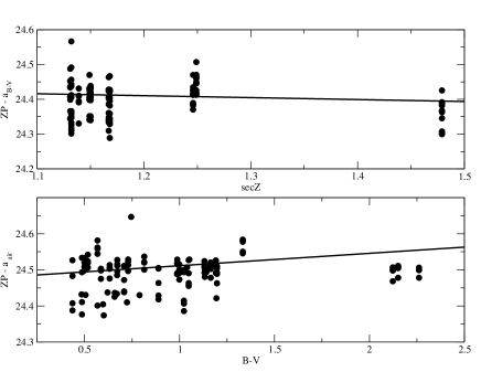
Figure 1: $V$-band standard star calibration for $3^{\rm rd}$ September 2000. Colour-corrected zero-points versus airmass (top) and airmass-corrected zero-points versus colour (bottom)

2.4 Object detection and photometry

Objects were detected automatically using the SExtractor package (Bertin & Arnouts 1996). SExtractor detects objects as groups of connected pixels which exceed a certain threshold. A criterion of 8 connected pixels above an isophotal threshold of $\mu_{0}=26.0$ mag arcsec^-2 was used. The best_mag parameter was used to measure total galaxy magnitude (hereafter denoted $V$); this corresponds to a Kron (1980) extraction aperture, except for crowed regions where an extrapolated isophotal magnitude is used. The Kron extraction aperture is set to 2.5 times $R_{K}$ where $R_{K}$ is the first moment of the image distribution. In regions where pointings overlap, the duplicate objects were removed from the catalogs.

2.5 Exclusion regions

After the initial object detection each field was visually inspected and any CCD defects, very bright stars, diffraction spikes and satellite trails causing spurious detections were identified. Circular and rectangular regions enclosing these areas were defined and excluded from the catalogs. In addition, the areas within 20 pixels of the CCD edge and the vignetted corner of CCD3 were also excluded.

2.6 Object classification

We used the position of objects in the central surface brightness–magnitude ($\mu_{o}$–$V$) plane to classify objects as either galaxies, stars or cosmic rays. The distribution of a subset of detected objects in this plane, for each cluster, is illustrated in Fig. 2. The central surface brightness was calculated in a circular aperture with an area equal to that of the detection criterion (i.e., 8 pixels).

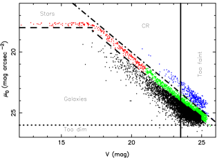
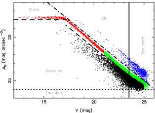
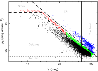
Figure 2: Distribution of detected objects in the central surface brightness–magnitude plane. Blue points are objects classified as cosmic rays, red points are objects classified as stars directly from their positions in this plane, green points are objects classified as stars by extrapolation from the brighter star counts and black points are the objects classified as galaxies. Top panel: A2218. Middle panel: A2443. Lower panel: A119. Only one in six objects, randomly selected, are displayed.

2.6.1 Cosmic ray rejection

In Fig. 2 a group of objects with a high central surface brightness (at a given magnitude) is clearly discernible (upper right). These objects, which have surface brightnesses higher than that of stars, are cosmic rays. We therefore define a region in the $\mu_{o}$–$V$ plane such that:

$$\mu_{o}\leq aV+b$$ (3)

and classify all objects in this region as cosmic rays. Equation (3) is shown as the dot-dashed line in Fig. 2. The slope ($a$) and intercept ($b$), were chosen separately for each cluster, to best match the data. The objects classified as cosmic rays are shown as blue points in Fig. 2.

2.6.2 Star-galaxy separation

The process of star-galaxy separation begins by identifying saturated stars in the catalogs. Stars brighter than $V\approx 17.2$ mag are saturated, these are clearly identifiable in the $\mu_{o}$–$V$ plane as a horizontal locus of points with $\mu_{o}<18.0$ mag arcsec^-2. We classify objects with:

$$\mu_{o}<18.0{\;\rm and\;}V\leq 17.2$$ (4)

as flooded stars (horizontal dashed line in Fig. 2). The stellar locus can be seen in Fig. 2 as a diagonal locus of points (red) with a higher surface brightness than the overall galaxy population (black points), and extending from $V\approx 17.2$ to $V\approx 21$ mag. We therefore define a line in the $\mu_{o}$–$V$ plane:

$$\mu_{o}=aV+b^{\prime}{\;\rm and\;}V>17.2{\;\rm and\;}V\leq 21.0$$ (5)

to pass between these populations, and we use it as a divider to separate stars and galaxies (see diagonal dashed line in Fig. 2). All objects with $V\leq 21$ mag which are classified as stars are shown in red in Fig. 2.

For objects fainter than $V\approx 21$ mag star-galaxy separation becomes problematic. At these magnitudes the stellar locus merges with that of the overall galaxy population and the two can no longer be distinguished. In order to perform star-galaxy classification faintward of $V=21$ mag we use a similar method to that outlined in Liske et al. (2003). Since the (logarithmic) slope of the star counts should remain roughly constant to $V\approx 24$ mag (Kümmel & Wagner 2001), we can use the star counts derived from the bright objects in the catalog and extrapolate them to derive the expected number of star counts at fainter magnitudes. We then classified objects as stars based on their position in the $\mu_{o}$–$V$ plane (objects with the lowest value of $\mu_{o}-mV$) until we had obtained the predicted number of stars. Although this method will result in some individual objects having incorrect classifications, the overall statistical proprieties of the catalogs will be correct. The objects that have been classified as stars in this way are shown in green in Fig. 2.

2.6.3 Completeness

At this point every object in the catalogs has been classified as either a star, galaxy or cosmic ray. We are limited to galaxies with a central surface brightness (over an area of 8 pixels) of $\mu_{o}\leq 26$ mag arcsec^-2 and from Fig. 2 we see that objects with central surface brightnesses close to this limit only occur in significant numbers at $V>23.5$ mag, indicating the beginning of detection incompleteness (Garilli et al. 1999). We therefore, define an apparent magnitude limit of $V=23.5$ mag.

3 Radial Profiles

The wide field-of-view provided by the WFC mosaics enable us to survey the radial distribution of galaxies beyond the domain of the cluster, well out into the surrounding field. To explore this, we plot for each cluster the galaxy-surface density against cluster-centric radius. This is achieved by deriving the galaxy counts in concentric annuli centred on the brightest cluster galaxy. The surface density was calculated taking into account the area of each annulus which encompasses the unmasked field-of-view of the available CCD area (i.e., corrected for any exclusion regions which intersect the annulus). We also corrected for the ‘diminishing area effect’ (Driver et al. 1998) whereby the area over which faint objects can be detected is reduced by the presence of brighter objects. To calculate this effect we used the SExtractor parameter ISOAREA – which returns the total area assigned to an object by SExtractor – to calculate the amount of area occupied by brighter objects.

The SExtractor best magnitudes were corrected for galactic extinction using the maps of Schlegel et al. (1998). The observed radial galaxy surface density profiles for A2218, A2443 and A119 are shown in Fig. 3, Fig. 4 and Fig. 5, respectively, as open squares. The error bars on the points are those expected from purely Poisson statistics.

Figure 3: The surface density of galaxies in A2218 as a function of cluster-centric radius for a series of magnitude intervals. The solid curves are the best fitting ‘King + constant’ profile given by equation (7). The (apparent) magnitude intervals and their corresponding absolute magnitude intervals (for the cluster redshift) as well as the best fitting values of the fit parameters are tabulated in each panel. The dashed lines show the value of the $N_{f}$ parameter from equation (7).

Figure 4: Same as Fig. 3 except for A2443

Figure 5: Same as Fig. 3 except for A119

3.1 Cluster profiles

The radial profiles in Figs. 3–5 represent the superposition of the cluster surface density profiles and a constant ‘field’ galaxy surface density. We elect to describe the cluster surface density in functional form by a King (1962) profile, plus a constant surface density of ‘field’ galaxies, thus:

$$\sigma(r)={\sigma_{0}\over 1+\bigl{(}{r\over r_{c}}\bigr{)}^{2}}+N_{f}$$ (6)

where $\sigma(r)$ represents the radially ($r$) dependent number-counts along the line-of-sight. The first term in equation (6) represents the projected distribution of cluster galaxies and the second term the superimposed ‘field’ population. In Figs. 3–5 we have binned the galaxy number counts in radial annuli. We therefore need to integrate our fitting function (equation 6) over the annuli to obtain the average surface density, which gives

$${1\over\pi(r_{max}^{2}-r_{min}^{2})}\int_{r_{min}}^{r_{max}}2\pi r\sigma(r)dr=$$

$$\left.{1\over r_{\rm max}^{2}-r_{\rm min}^{2}}\left[N_{f}r^{2}+\sigma_{0}r_{c}^{2}\log{(1+(r/r_{c})^{2})}\right]\right|_{r_{\rm min}}^{r_{\rm max}}$$ (7)

where $r_{min}$ and $r_{max}$ are the inner and outer radial boundaries of the bin, respectively. The fitted profiles to the measured galaxy surface density profiles are shown as the solid lines in Fig. 3–5 in 1 mag intervals of $V$. Overall, the surface density of galaxies are well described by equation (6).

In Fig. 6 we show the King profile core radii [given by the parameter $r_{c}$ in equation (7)] as a function of absolute $V$-band magnitude, the errors on the points are calculated directly from the covariance matrix returned from $\chi^{2}$ minimisation. In the case of the clusters A2443 (middle panel) and A119 (lower panel) we find that the core radius is essentially independent of magnitude, with both clusters having core radii of $r_{c}\approx$ 0.2–0.5 Mpc at all luminosities. The best fitting slopes are given by $-0.001\pm 0.033$ Mpc mag^-1 and $0.058\pm 0.040$ Mpc mag^-1, respectively – both consistent with zero at $\sim 1\sigma$. In A2218, we find that the brightest galaxies have a smaller core radius then their fainter counterparts, with marginal evidence that this trend – increasing core radius with decreasing luminosity – continues for the intermediate population. The best fitting slope is given by $0.086\pm 0.030$ Mpc mag^-1. However, if the brightest points ($M_{V}<-21$ mag) are removed, the slope becomes $0.051\pm 0.054$ Mpc mag^-1 which is consistent with zero at less than the $1\sigma$ level. This trend is generally consistent with Pracy et al. (2004) who found that the spatial distribution of galaxies in A2218 is more extended for the lower luminosity populations. Unfortunately the data do not extend to their dwarf and ultra-dwarf regimes.

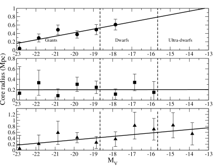
Figure 6: Core radii [$r_{c}$ from equation (7)] versus absolute $V$-band magnitude. Top panel: A2218. Middle panel: A2443. Lower panel: A119. The best fitting slopes are displayed as solid lines. The ‘Giant’, ‘Dwarf’ and ‘Ultra-dwarf’ regimes, as defined by Pracy et al. (2004), are delineated by the dashed lines. These definitions have been adjusted due to differences in the filters and the assumed cosmology.

3.2 Reference field counts

In order to study the cluster galaxy population we need to remove the contribution to the counts along the line-of-sight from foreground and background ‘field’ galaxies. To do this we use the standard technique of statistical field subtraction. However rather than use data obtained from off-cluster pointings we are now able to use the counts derived from the radial fits (i.e., $N_{f}$ in equation 7).

The field galaxy number counts derived in this way are shown in the top panel of Fig. 7, where we have plotted the counts from the A2218 field (filled squares), the A2443 field (filled circles) and the A119 field (stars), separately. For comparison we also plot the galaxy number counts from the Millennium Galaxy Catalog (MGC) of Liske et al. (2003), which we have converted from the $B$-band to the $V$-band using the mean field galaxy colour $(B-V)=0.94$ (Norberg et al. 2002). We note that this colour is only strictly valid for $V<18$ mag; however, the number counts agree quite well over the entire range of luminosities. The ‘field’ counts derived for the low redshift cluster A119 generally have larger error bars and much larger scatter than those derived for the other two clusters. This is expected since the radial profiles for this cluster extend to a radius of only $\sim 2$ Mpc. The scatter in the points can be seen more clearly in the lower panel of Fig. 7 where we show the galaxy counts relative to a $N\propto 10^{0.45V}$ relation.

Figure 7: Top: ‘field’ galaxy counts derived from equation (7, see text for details); filled squares are the reference ‘field’ counts from the A2218 field; filled circles for the A2443 field and stars for the A119 field. The open triangles are the ‘field’ galaxy counts from the MGC. The solid line is a quadratic fit to the counts from all three clusters. Bottom: ‘field’ galaxy counts shown relative to a $10^{0.45V}$ relation. The quadratic fits to the counts are shown as the solid line (A2218), dashed line (A2443) and dot-dash line (A119).

In order to give a smooth representation of the ‘field’ counts we fitted a quadratic function to them. Since ‘field’ galaxy counts can vary significantly between fields, a quadratic fit was performed separately for each set of reference ‘field’ counts. These fits are shown in the lower panel of Fig. 7 as the solid, dashed and dot-dashed lines for A2218, A2443 and A119, respectively. For illustrative purposes a simultaneous fit to all three data sets is shown as the solid line in the top panel of Fig. 7. We also used the MGC counts at $V<18$ mag to provide a bright end ‘anchor’ to the fit – we artificially introduced errors of 10% on these points so as not to allow the MGC points to influence the fit at the critical faint end. The quadratic fits yield:

$${dN\over dV} =10^{a+bV+cV^{2}}$$

$$a =-7.83486,-7.64871,-10.87945$$

$$b =0.6404656,0.6162334,0.9579601$$

$$c =-0.0052439445,-0.0044137863,-0.0130500505$$

(for A2218, A2443, A119, respectively). We use these analytical representations of the ‘field’ counts, adjacent to each cluster, for statistical field subtraction throughout. We note that this method will also correct, in a statistical sense, for any incompleteness in the cosmic ray rejection.

Since we will use the analytic representation of the ‘field’ counts given in equation (3.2) to remove contamination by ‘field’ galaxies superimposed on the cluster, we require an estimate of the uncertainty in this analytic representation. To do this we use the formal variances and covariances for each of the fit parameters ($a$, $b$ and $c$) returned from the $\chi^{2}$ minimization. The error ($\epsilon$) on the ‘field’ counts is given by:

$$\epsilon^{2}=\left({dN\over dV}\ln 10\right)^{2}\left(\delta_{a}^{2}+V^{2}\delta_{b}^{2}+V^{4}\delta_{c}^{2}\right.$$

$$\left.+2V\delta_{ab}+2V^{2}\delta_{ac}+2V^{3}\delta_{bc}\right)$$ (9)

where $dN\over dV$ is the number of galaxies per magnitude interval [given by equation (3.2)] centred on apparent magnitude $V$. $\delta_{a}^{2}$, $\delta_{b}^{2}$ and $\delta_{c}^{2}$ are the variances and $\delta_{ab}$, $\delta_{ac}$ and $\delta_{bc}$ are the covariances on the fitted parameters $a$, $b$ and $c$.

3.3 Lensing

A possible concern regarding the background counts is the impact of lensing by the cluster mass. This consists of two effects: a magnification effect whereby the background population is brightened, and a tangential compression of the the background volume. While the former can increase the counts, the latter can decrease it (i.e., the effect is to narrow and lengthen the observable volume behind the cluster). The precise details of this correction are given by Trentham (1998) and Bernstein et al. (1995).

In Fig. 8 we plot the fractional change in the observed number of ‘field’ galaxy counts caused by lensing, $f_{lens}$, as a function of $V$-band magnitude for each cluster – averaged over the central 500 kpc. That is, the ratio of the number of ‘field’ galaxies observed at a given magnitude viewed along the cluster line-of-sight to the number of galaxies expected if not observed through the cluster lens. In modelling the lensing effect we follow the procedure outlined in Pracy et al. (2004) and references therein. We use a value for the velocity dispersion of 1370 km s^-1 for A2218 (Le Borgne et al. 1992) and 778 km s^-1 for A119 (Struble & Rood 1987); since no velocity data is available for A2443 we assume a velocity dispersion for this cluster of 1000 km s^-1. We use the local luminosity function measured from the MGC (Driver et al. 2005) and convert to the $V$-band using $B-V=0.94$ (Norberg et al. 2002).

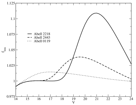
Figure 8: The function $f_{lens}$ averaged over the central 500 kpc for A2218 (solid line), A2443 (dashed line) and A119 (dotted line).

In Fig. 8 the function $f_{lens}$ is shown for A2218 as the solid line, for A2443 as the dashed line and for A119 as the dotted line. Clearly, the effect is largest for A2218, primarily as a result of the cluster’s higher redshift. In A2218 the effect is most evident for galaxies with $V\approx 21$ with a fractional change in the ‘background’ population of approximately 10%. At this level the lensing effect represents a minor component of the error budget. However it is worth noting that the lensing correction depends critically on the assumptions concerning the evolution of the galaxy number counts as a function of redshift, which is not well known. Given this uncertainty and the small size of the corrections in Fig. 8, we do not correct for lensing at this time.

4 Luminosity functions

We now use our data along with our measured ‘field’ counts to study the luminosity distribution of galaxies in each cluster. The faint–end limits for A2218, A2443 and A119 are, respectively, $M_{V}=-16.7$, $M_{V}=-15.4$ and $M_{V}=-13.3$ mag. These include correction for galactic dust (Schlegel et al. 1998) and K-correction (Poggianti 1997).

4.1 Central luminosity distribution

We first construct, for each cluster, the luminosity distribution of galaxies within a cluster-centric radius of 1 Mpc. We use equation (3.2) – scaled to the appropriate area – to correct ‘statistically’ for contamination by the superimposed ‘field’ galaxy population. These are shown in the left panels of Fig. 9 for A2218 (top), A2443 (middle) and A119 (bottom) – and are also tabulated in Table 2. We fit each of the luminosity distributions with a Schechter (1976) function; which has been convolved with the magnitude bin width. The luminosity distributions in all three clusters are well described by a Schechter function with shape parameters $M^{*}_{V}=-21.54_{-0.11}^{+0.14}$ and $\alpha=-1.14_{-0.07}^{+0.08}$ for A2218, $M^{*}_{V}=-21.32_{-0.36}^{+0.39}$ and $\alpha=-1.11_{-0.09}^{+0.10}$ for A2443 and $M^{*}_{V}=-21.51_{-0.20}^{+0.30}$ and $\alpha=-1.22_{-0.06}^{+0.07}$ for A119. Since the parameters $M^{*}$ and $\alpha$ are dependent we plot, in the right hand panels of Fig. 9, the $1$, $2$ and $3\sigma$ error contours for the Schechter function fit.

Figure 9: Left panels: The luminosity distributions for the clusters A2218 (top), A2443 (middle) and A119 (bottom) within a cluster-centric radius of 1 Mpc. The data are shown by the stars and the solid line is a Schechter (1976) function fit to the data. The right panels show the $1$, $2$ and $3\sigma$ error ellipses for the Schechter function parameters $M^{*}$ and $\alpha$. Also shown (open circle in top panel) is the best–fitting Schechter function parameters for the ‘bright-end’ of the luminosity distribution of A2218 from Pracy et al. (2004).

Table 2: luminosity distributions

Cluster	Mag interval	Counts	Error
A2218	$-23.68<M_{V}\leq-22.68$	2.19	1.73
”	$-22.68<M_{V}\leq-21.68$	26.67	5.39
”	$-21.68<M_{V}\leq-20.68$	60.48	8.19
”	$-20.68<M_{V}\leq-19.68$	82.16	10.00
”	$-19.68<M_{V}\leq-18.68$	103.37	12.29
”	$-18.68<M_{V}\leq-17.68$	138.87	16.22
”	$-17.68<M_{V}\leq-16.68$	212.23	22.98
A2443	$-23.39<M_{V}\leq-22.39$	0.42	1.00
”	$-22.39<M_{V}\leq-21.39$	16.28	4.24
”	$-21.39<M_{V}\leq-20.39$	31.01	6.00
”	$-20.39<M_{V}\leq-19.39$	47.78	7.87
”	$-19.39<M_{V}\leq-18.39$	66.31	10.30
”	$-18.39<M_{V}\leq-17.39$	100.41	14.46
”	$-17.39<M_{V}\leq-16.39$	99.91	19.78
”	$-16.39<M_{V}\leq-15.39$	73.38	28.96
A119	$-23.31<M_{V}\leq-22.31$	1.80	1.41
”	$-22.31<M_{V}\leq-21.31$	12.24	3.61
”	$-21.31<M_{V}\leq-20.31$	32.24	5.92
”	$-20.31<M_{V}\leq-19.31$	66.54	8.72
”	$-19.31<M_{V}\leq-18.31$	63.48	9.72
”	$-18.31<M_{V}\leq-17.31$	65.33	12.72
”	$-17.31<M_{V}\leq-16.31$	111.00	20.16
”	$-16.31<M_{V}\leq-15.31$	173.38	32.21
”	$-15.31<M_{V}\leq-14.31$	200.41	49.05
”	$-14.31<M_{V}\leq-13.31$	254.88	78.41

The luminosity distribution of galaxies in A2218 has been studied by Pracy et al. (2004) using a deep HST mosaic of the cluster. Their ‘bright-end’ luminosity distribution is comparable in bandpass, areal coverage and luminosity range to the one derived above – with a projected area covered of $\sim 2.6\,h^{-2}_{0.7}$ Mpc² (compared with $\sim 3.1\,h^{-2}_{0.7}$ Mpc² in this study) and a luminosity range corresponding to $M_{V}<-17$ (compared with $M_{V}<-16.7$ here). Here we have converted to the $V$-band using the relation $V=F606W+0.12$ (Norberg et al. 2002; Driver et al. 2003) and corrected for differences in assumed cosmology, dust extinction, K-correction, and the omission of the cD galaxy in Pracy et al. (2004). We show the best–fitting Schechter function parameters from Pracy et al. (2004) along with the error contours in Fig. 9. The recovered Schechter function parameters are in good agreement ($-1.23\pm 0.09$ cf. $\alpha=-1.14_{-0.07}^{+0.08}$ in this study and $M^{*}_{V}=-21.85\pm 0.46$ compared with $M^{*}_{V}=-21.54_{-0.11}^{+0.14}$ here).

Table 3: Recent measurements of the LF parameters from wide–field $V$-band CCD photometry

Cluster	redshift	Area (Mpc2)	Magnitude range	$M_{V}^{*}$	$\alpha$	Reference
Coma$\dagger$	0.023	$\sim 0.9$	$-21.51<M_{V}<-11.51$	NA	$-1.43_{-0.03}^{+0.06}$	Andreon & Cuillandre (2002)
Coma	0.023	$\sim 1.1$	$-21.51<M_{V}<-14.01$	NA	$-1.59\pm 0.02$	Lobo et al. (1997)
Abell 2151	0.037	$\sim 8.3$	$M_{V}<-15.0$	$-21.56_{-0.41}^{+0.44}$	$-1.29_{-0.08}^{+0.09}$	Sánchez-Janssen et al. (2005)
Abell 119	0.044	$\sim 3.1$	$M_{V}<-13.3$	$-21.51_{-0.20}^{+0.30}$	$-1.22_{-0.06}^{+0.07}$	This work
Abell 2443	0.108	$\sim 3.1$	$M_{V}<-15.4$	$-21.32_{-0.36}^{+0.39}$	$-1.11_{-0.09}^{+0.10}$	This work
Abell 2218	0.181	$\sim 3.1$	$M_{V}<-16.7$	$-21.54_{-0.11}^{+0.14}$	$-1.14_{-0.07}^{+0.08}$	This work
ABCG 209	0.209	$\sim 3.4$	$M_{V}<-17.6$	$-22.18\pm 0.3$	$-1.27\pm 0.10$	Mercurio et al. (2003)
ABCG 209	0.209	$\sim 6.9$	$M_{V}<-17.6$	$-22.03\pm 0.3$	$-1.25\pm 0.08$	Mercurio et al. (2003)
AC 118	0.310	$\sim 5.5$	$M_{V}<-18.2$	$-20.93\pm 0.4$	$-1.02\pm 0.18$	Busarello et al. (2002)

$\dagger$ Based on a Schechter function fit to on-line data

In Table 3 we tabulate the results of recent wide–field $V$-band LF studies: column (1) identifies the cluster, column (2) gives the cluster redshift, column (3) gives the total area covered, column (4) indicates the absolute magnitude limits of the data, column (5) presents the characteristic magnitude, column (6) gives the value of the faint–end–slope parameter, and column (7) identifies the reference. All values have been converted to an ${\Omega}_{M}=0.3$, ${\Omega}_{\Lambda}=0.7$ and $H_{0}=70$ km s^-1 Mpc^-1 cosmology. Although, comparison of the LF parameters is somewhat complicated by differences in redshift (and hence rest-frame bandpass), areal coverage, and the magnitude limits of the data – the values, and the precision, of the LF parameters presented here are comparable to those given in the literature. However, we derive faint–end–slope parameters for these clusters which are marginally flatter than the average. With the exception of Andreon & Cuillandre’s (2002) Coma LF, our Abell 119 data represents the deepest determination of a wide–field $V$-band LF available.

4.2 Composite luminosity distribution

We now construct a composite luminosity distribution from our three clusters. To do this we average the background–subtracted number counts in each magnitude bin normalised by the cluster’s ‘richness’:

$$\zeta(M)={\sum_{i=1}^{n_{\rm c}}N_{i}(M)\over\sum_{i=1}^{n_{\rm c}}R_{i}},$$ (10)

where $\zeta(M)$ is the combined galaxy number ‘counts’ in the magnitude interval centred on $M$, $n_{\rm c}$ is the number of clusters in the composite luminosity distribution ($n_{\rm c}=3$) and $N_{i}(M)$ is the galaxy number counts in the magnitude bin centred on $M$ for the $i$th cluster. $R_{i}$ is the ‘richness count’ of the $i$th cluster, which is taken to be the total number of background–subtracted galaxies in the magnitude range $-21<M_{V}<-19$ within a cluster-centric radius of $1.5\;h_{0.7}^{-1}$ Mpc (Valotto et al. 2001).

The composite luminosity distribution and best–fitting Schechter function (solid line) is shown in Fig. 10. The shape of the best–fitting Schechter function is parameterised by $M^{*}_{V}=-21.82_{-0.18}^{+0.21}$ and $\alpha=-1.22_{-0.04}^{+0.05}$. The $1$, $2$ and $3\sigma$ error contours of the parameters $M^{*}_{V}$ and $\alpha$ for our composite luminosity distribution are shown in the right panel of Fig. 10, along with the positions in the $M^{*}_{V}$–$\alpha$ plane of a subsample of the composite luminosity function parameters from the literature (converted to the $V$-band). The open circle and star represent the field galaxy luminosity functions derived from the MGC (Driver et al. 2005) and Two Degree Field Galaxy Redshift Survey (2dFGRS; Colless et al. 2001), both of which exhibit faint–end slopes ($\alpha$) that are similar to that of our composite luminosity function but have a brighter and fainter characteristic magnitude ($M^{*}$), respectively. The open square represents the best–fitting Schechter function parameters for a composite of clusters (De Propris et al. 2003) drawn from the 2dFGRS with a mean redshift of $z=0.12$. Our composite luminosity function has a marginally brighter characteristic magnitude to that of the 2dFGRS cluster composite and a slightly flatter $\alpha$. The open triangle shows the formal Schechter function parameters from Goto et al. (2002) for a composite of clusters in the redshift range $0.2<z<0.25$ from the Sloan Digital Sky Survey, which has a significantly brighter characteristic magnitude and flatter faint–end slope.

Figure 10: Left panel: The composite luminosity function of the three clusters. Right panel: the $1$, $2$ and $3\sigma$ error ellipses with a set of Schechter function parameters for composite luminosity functions from the literature superimposed. See text for details.

5 Geometric deprojection

The wide field-of-view of the WFC mosaics provides coverage of the entire cluster area, in the sense that the number of galaxies per unit area no longer decreases with radius at the outermost regions covered by the imaging.

We use the scheme of Fabian et al. (1981, see ) to perform geometric deprojection of the clusters. The projected cluster galaxy population is separated into a set of concentric annuli within which the galaxy density is assumed to be constant. The deprojection scheme assumes the cluster galaxies are distributed spherically symmetrically so that the projected number of galaxies in each annulus corresponds to a real galaxy number density in the corresponding spherical shell. The number density in each shell can then be corrected for the projection of galaxies from all shells of greater radius, beginning with the outermost shell and iteratively moving inward.

The projected galaxy density for each magnitude bin, $m$, in the $i$th annulus, $N_{i,m}$, is given by:

$$N_{i,m}=\phi_{i,m}F(R_{i},R_{i-1},R_{i})+$$

$$\sum_{j=i+1}^{n}\phi_{j,m}(F(R_{j},R_{i-1},R_{i})-F(R_{j-1},R_{i-1},R_{i}))$$ (11)

where the $R_{i}$’s are the radii of the annuli, $\phi_{i,m}$ is the 3D galaxy density and the function $F$ is defined by:

$$F(\alpha,\beta,\gamma)={4\over 3}\pi\alpha^{3}\biggl{(}\biggl{(}1-{\beta^{2}\over\alpha^{2}}\biggl{)}^{3/2}-\biggl{(}1-{\gamma^{2}\over\alpha^{2}}\biggl{)}^{3/2}\biggl{)}$$ (12)

(Beijersbergen et al. 2002).

We set radial bin partitions at cluster-centric radii of 0.3, 0.6 and 1.5 Mpc – splitting the cluster field into four regions ($n=4$) – and perform geometric deprojection of the data in 1 magnitude intervals. We first subtract from the number counts in each annuli the contribution from the superimposed field galaxy population using equation (3.2) – normalised to the area of ‘detectability’ for each annulus. We use the outermost annuli ($R>1.5$ Mpc) to begin the deprojection, that is, set $i=3$ in equation (5) and then iteratively calculate the deprojected (3-Dimensional) luminosity function in each of the inner three annuli: $0.0\,{\rm Mpc}<r<0.3\,{\rm Mpc}$, $0.3\,{\rm Mpc}<r<0.6\,{\rm Mpc}$ and $0.6\,{\rm Mpc}<r<1.5\,{\rm Mpc}$. The errors in the 3D galaxy density are calculated by propagating the appropriate galaxy–count and field–subtraction errors through equation (5).

The deprojected 3D luminosity functions are shown in Fig. 11 for A2218 (top), A2443 (middle) and A119 (bottom). The open circles, open squares and open triangles are the galaxy densities in the inner, middle and outer annuli, respectively, and the solid, dashed and dotted lines show their best fitting Schechter functions. The $1$, $2$ and $3\sigma$ error contours for the Schechter function shape parameters $M_{V}^{*}$ and $\alpha$ are shown in the right hand panels of Fig. 11. The core region ($r<300$ kpc) of A2218 has a LF with a flatter faint–end slope than the LFs measured at larger cluster-centric radii within this cluster, while the other clusters show no significant systematic correlation with cluster-centric radius. A summary of the Schechter function fit parameters are given in Table 4.

Table 4: Schechter function parameter values for the deprojected (3-dimensional) luminosity functions in three annuli: $0.0\,{\rm Mpc}<r<0.3\,{\rm Mpc}$, $0.3\,{\rm Mpc}<r<0.6\,{\rm Mpc}$ and $0.6\,{\rm Mpc}<r<1.5\,{\rm Mpc}$

Cluster	Radius (Mpc)	$M_{V}^{*}$	$\alpha$
A2218	0–0.3	$-22.12_{-0.57}^{+0.57}$	$-0.94_{-0.16}^{+0.19}$
	0.3–0.6	$-22.31_{-0.77}^{+0.60}$	$-1.30_{-0.15}^{+0.16}$
	0.6–1.5	$-21.86_{-0.35}^{+0.37}$	$-1.36_{-0.10}^{+0.11}$
A2443	0–0.3	$-20.72_{-0.63}^{+0.58}$	$-1.00_{-0.19}^{+0.22}$
	0.3–0.6	$-21.72_{-0.63}^{+0.72}$	$-1.19_{-0.12}^{+0.14}$
	0.6–1.5	$-20.03_{-0.88}^{+1.02}$	$-1.01_{-0.18}^{+0.45}$
A119	0–0.3	$-22.24_{-1.78}^{+1.54}$	$-1.25_{-0.11}^{+0.16}$
	0.3–0.6	$-21.53_{-0.70}^{+0.71}$	$-1.16_{-0.12}^{+0.16}$
	0.6–1.5	$-21.66_{-0.54}^{+0.51}$	$-1.23_{-0.10}^{+0.12}$

Figure 11: Left panels: the deprojected luminosity distributions of galaxies in cluster-centric annuli of 0–0.3 Mpc (open circles), 0.3–0.6 Mpc (open squares) and 0.6–1.5 Mpc (open triangles) and their best fitting Schechter functions (solid, dashed and dotted lines, respectively). Right panels: $1$, $2$ and $3\sigma$ error contours for the Schechter function parameters $M_{V}^{*}$ and $\alpha$. A2218: top panel, A2443: middle panel and A119: bottom panel.

6 Summary and Discussion

We have exploited wide–field imaging of three galaxy clusters to examine the luminosity and spatial distribution of their member galaxies and to search for evidence of luminosity segregation. We cover a total projected area which corresponds to 120.5 Mpc², 50.4 Mpc² and 9.7 Mpc² in A2218, A2443 and A119, respectively. We find that the radial distribution of galaxies can be well described by a King profile with a core radius which is essentially independent of luminosity – the exception being the brightest galaxies in A2218 which exhibit a more compact spatial distribution. Galaxies at different luminosities having the same spatial distribution, of course, indicates that no luminosity segregation is present. We find, in all three clusters, a luminosity distribution of galaxies which is well described by a Schechter function with a flat faint–end slope ($\alpha\sim-1.2$). We have performed a geometric deprojection of the cluster population. The luminosity function remains flat after deprojection and (except for the core region of A2218) we find no statistically significant evidence for any change with cluster-centric radius – consistent with our radial profile analysis.

The segregation of galaxies of different luminosities is a key prediction of hierarchical models of galaxy formation and evolution. The numerical CDM models of Kauffmann et al. (1997), for example, predict that low luminosity galaxies should be less clustered than the bright ‘giant’ galaxies (see Phillipps et al. 1998). Evolutionary mechanisms operating in clusters which should give rise to luminosity segregation have also been suggested. Moore et al. (1998) have been able to explain the dwarf population–density relation (in which the ratio of dwarf galaxies to giant galaxies increases with decreasing local galaxy density) as the result of galaxy ‘harassment’ – which operates more effectively in regions of high galaxy density. Interaction with the cluster tidal field will destroy the lowest surface brightness (least bound) objects in the central region of a cluster, resulting in a deficiency of faint galaxies in the cluster core. If luminosity segregation in clusters is not present then the impact of these effects on the low-luminosity cluster galaxies has been exaggerated.

The key issue in searching for luminosity segregation in clusters is that of the technique of background subtraction employed. The fractional difference between the total (cluster+‘field’) galaxy counts and the ‘field’ galaxy counts decreases with decreasing luminosity. Therefore, any systematic error in the estimate of the field galaxy counts can mimic both a faint–end upturn in the luminosity function and luminosity segregation – in the sense that underestimating the field counts will result in a larger fraction of faint galaxies at low local galaxy densities. Using spectroscopy to confirm cluster membership is essentially useless for all but the nearest clusters, since the galaxies at the critical faint end of the luminosity function are too faint for spectroscopic confirmation. Hence, most often a statistical subtraction of the field is performed using galaxy counts measured from a region offset from the cluster line-of-sight. Valotto et al. (2001) point out one possible source of bias in statistical field subtraction due to the alignments between filaments and clusters which can result in an underestimate of the ‘field’ galaxy population. Here we have used an analytic representation (equation 6) of the radial distribution of galaxies toward the cluster sight-line to simultaneously obtain the cluster profile and the superimposed ‘field’ galaxy surface density. Note, fitting equation (6) to the radial profiles in Fig. 3, Fig. 4 and Fig. 5 does not require prior subtraction of the field galaxy population and we, therefore, suggest that this is a superior test for luminosity segregation. Very recently Andreon et al. (2005) have suggested an alternative method to alleviate and quantify the problems of background subtraction in deriving cluster luminosity functions – a detailed comparison of these methods and the traditional method should be pursued in a future paper.

References

- Andreon (2002) Andreon S., 2002, A&A, 382, 821
- Andreon & Cuillandre (2002) Andreon S., Cuillandre J.-C., 2002, ApJ, 569, 144
- Andreon et al. (2005) Andreon S., Punzi G., Grado A., 2005, MNRAS, 360, 727