Reconciling the local galaxy population with damped Ly $\alpha$ cross-sections and metal abundances

Abstract

A comprehensive analysis of 355 high-quality WSRT H i 21-cm line maps of nearby galaxies shows that the properties and incident rate of Damped Lyman $\alpha$ absorption systems (DLAs) observed in the spectra of high redshift QSOs are in good agreement with DLAs originating in gas disks of galaxies like those in the $z\approx 0$ population. Comparison of low $z$ DLA statistics with the H i incidence rate and column density distribution $f(N_{\rm HI})$ for the local galaxy sample shows no evidence for evolution in the integral “cross section density” $<n\sigma>=l^{-1}$ ($l$=mean free path between absorbers) below $z\approx 1.5$, implying that there is no need for a hidden population of galaxies or H i clouds to contribute significantly to the DLA cross section. Compared with $z\approx 4$, our data indicates evolution of a factor of two in the comoving density along a line of sight. We find that $dN/dz(z=0)=0.045\pm 0.006$. The idea that the local galaxy population can explain the DLAs is further strengthened by comparing the properties of DLAs and DLA galaxies with the expectations based on our analysis of local galaxies. The distribution of luminosities of DLA host galaxies, and of impact parameters between QSOs and the centres of DLA galaxies, are in good agreement with what is expected from local galaxies. Approximately 87 per cent of low $z$ DLA galaxies are expected to be fainter than $L_{*}$ and 37 per cent have impact parameters less than 1^′′ at $z=0.5$. The analysis shows that some host galaxies with very low impact parameters and low luminosities are expected to be missed in optical follow up surveys. The well-known metallicity–luminosity relation in galaxies, in combination with metallicity gradients in galaxy disks, cause the expected median metallicity of low redshift DLAs to be low ($\sim$1/7 solar), which is also in good agreement with observations of low $z$ DLAs. We find that $f(N_{\rm HI})$ can be fitted satisfactorily with a gamma distribution, a single power-law is not a good fit at the highest column densities $\mbox{$N_{\rm HI}$}>10^{21}~{}\mbox{$\rm cm^{-2}$}$. The vast majority ($\approx 81$ per cent) of the H i gas in the local Universe resides in column densities above the classical DLA limit ($\mbox{$N_{\rm HI}$}>2\times 10^{20}\mbox{$\rm cm^{-2}$}$), with $\mbox{$N_{\rm HI}$}\sim 10^{21}\mbox{$\rm cm^{-2}$}$ dominating the cosmic H i mass density.

1 Introduction

How does the cosmological mass density of neutral hydrogen (H i) gas evolve over the history of the Universe and what sort of galaxies are responsible for this evolution? Two completely unrelated observational techniques are used to find answers to these questions for the present epoch and at earlier cosmic times. At intermediate and high redshifts (out to $z\sim 6$) deep optical and UV spectra of background quasars are scrutinised to find high column density H i that causes optical depth $\tau_{\rm LL}\ga 1$ blueward of the Lyman limit. In detecting these absorbing systems, their distance is not a limiting factor since the detection depends only on the brightness of the background source against which the absorber is found. However, the nature of the absorbing system is difficult to determine because the absorption spectrum only gives information along a very narrow sight-line through the system. Despite the large effort that has been dedicated to identify and characterise the high redshift absorbers through deep optical imaging, very little about their properties is yet known (e.g., Møller et al., 2002, and references therein).

At $z=0$, 21-cm emission line surveys are used to study the high column density H i. Blind surveys with the Arecibo and Parkes radio telescopes have resulted in accurate measurements of the cosmic H i mass density $\mbox{$\Omega_{\rm HI}$}(z=0)$ (Zwaan et al., 1997; Rosenberg & Schneider, 2002; Zwaan et al., 2003, 2005). In contrast to the high redshift studies, the 21-cm emission line surveys readily result in measurements of the total H i masses of the detected objects. Furthermore, after follow-up with an aperture synthesis instrument, the 3-dimensional H i data cube can be obtained, from which a detailed velocity field and column density map can be derived. Unfortunately, the H i 21-cm hyperfine line is very weak, which limits the studies to the very local Universe ($z<0.2$). The column densities that routine 21-cm emission line observations can sense, are the same as those of the highest column density Ly$\alpha$ absorbers known as Damped Ly$\alpha$ systems, or DLAs, with column densities $\mbox{$N_{\rm HI}$}>2\times 10^{20}\,\mbox{$\rm cm^{-2}$}$. These are the systems that contain most of the cosmic H i mass (e.g., Wolfe et al. , 1986; Lanzetta et al., 1991; Storrie-Lombardi & Wolfe, 2000), although there are indications that systems with slightly lower column densities may contribute approximately 20 per cent to $\Omega_{\rm HI}$ (Péroux et al., 2005).

The purpose of this paper is to test whether the results from the $z=0$ 21-cm line surveys and the $z>0$ UV and optical surveys can be reconciled. This question relates directly to the problem of the origin of DLA systems. Traditionally, DLAs were thought to arise in large gaseous disks in the process of evolving to present-day spiral galaxies (Wolfe et al. , 1986, 1995). This idea was supported by the fact that the velocity profiles of unsaturated, low-ion metal lines are consistent with rapidly rotating, large thick disks (Prochaska & Wolfe, 1997, 1998). Dissenting views do exist, perhaps most notably presented by Haehnelt, Steinmetz, & Rauch (1998), who argued that the velocity structure can alternatively be explained by protogalactic clumps coalescing on dark matter haloes (see also Ledoux et al., 1998; Khersonsky & Turnshek, 1996). In this view, the DLA systems are aggregates of dense clouds with complex kinematics rather than ordered rotating gas disks.

Imaging surveys for DLA host galaxies have so far not resulted in a consistent picture of their properties (Le Brun et al., 1997; Fynbo, Møller, & Warren, 1999; Kulkarni et al., 2000; Bouché et al., 2001; Warren et al., 2001; Colbert & Malkan, 2002; Møller et al., 2002; Prochaska et al., 2002; Rao et al., 2003; Lacy et al., 2003; Chen & Lanzetta, 2003). The few successful identifications show that a mixed population of galaxies is responsible for the DLA cross section. Semi-analytical and numerical models of galaxy formation point to sub-$L_{*}$ galaxies as the major contributors to H i cross section above the DLA limit (e.g., Kauffmann, 1996; Gardner et al., 2001; Nagamine, Springel, & Hernquist, 2004; Okoshi & Nagashima, 2005).

In this paper we concentrate primarily on cross-section arguments. Burbidge et al. (1977) started the discussion on whether the disks of normal galaxies can explain the incidence rate of absorbers. The method consists of multiplying the space density of galaxies (measured through the optical luminosity function) with the average area of the H i disk above the DLA column density limit. Burbidge et al. (1977) concluded that the mean free path for interception with a galactic disk was too large to account for the number of observed absorbers. Wolfe et al. (1986), Lanzetta et al. (1991), Fynbo, Møller, & Warren (1999), Schaye (2001), and Chen & Lanzetta (2003) use variations of this same simple analytical approach for estimates at high and low $z$. Although these approaches are useful to gain insight in the problem, a much more direct method is to use real 21-cm column density maps of local galaxies to evaluate the DLA incidence rate. This method was first used by Rao & Briggs (1993) who used Gaussian fits to the radial H i distribution of 27 galaxies as measured with the Arecibo Telescope. Much higher resolution H i maps were used by Zwaan, Briggs, & Verheijen (2002) who used WSRT maps of a volume-limited sample of 49 galaxies in the Ursa Major cluster (Verheijen & Sancisi, 2001). A similar study was conducted by Ryan-Weber, Webster, & Staveley-Smith (2003) based on 35 galaxies selected from HIPASS (Meyer et al., 2004), which were observed with the ATCA. Finally, Rosenberg & Schneider (2003) used low-resolution ($\sim 45^{\prime\prime}$) VLA maps of their sample of 50 H i-selected galaxies.

With the completion of WHISP (The Westerbork H i survey of Spiral and Irregular galaxies, van der Hulst, van Albada, & Sancisi 2001) we have available a much larger sample of galaxies, with a high dynamic range in galaxy properties and observed with a spatial resolution of $\approx 12^{\prime\prime}\times 12^{\prime\prime}/\sin\delta$. With this sample, the cross section analysis can be done more accurately and in more detail. This paper is organised as follows. In the following section we describe the details of the WHISP sample, in section 3 we summarise surveys for low redshift DLA host galaxies and compile a sample of these systems that we use for our comparison with $z=0$. We calculate the H i column density distribution function in section 4 and compare the results with the statistics at higher redshifts in section 5. A comparison of the redshift number density $dN/dz$ between $z=0$ and higher redshift is given in section 6. In section 7 we calculate the probability distribution functions of various parameters of cross-section selected galaxy samples and show that these agree well with results of low-$z$ DLA host galaxy searches. In Section 8 we show that the observed metallicities in DLAs are in good agreement with the expected values if low-$z$ DLAs arise in the gas disks of galaxies typical of the $z=0$ population. Section 9 summarises the results. We use $H_{0}=75~{}\mbox{$\rm km\,s^{-1}\,Mpc^{-1}$}$ throughout this paper to calculate distance dependent quantities.

2 The WHISP sample

The incidence rate of high column density H i in the local Universe can best be calculated from 21-cm maps of a large sample of galaxies with uniform selection criteria and high spatial resolution. Such a sample is available through WHISP (The Westerbork H i survey of Spiral and Irregular galaxies, van der Hulst, van Albada, & Sancisi 2001), an H i survey of some 390 galaxies carried out with the Westerbork Synthesis Radio Telescope in the periods 1992 to 1998 and 2000 to 2002. The aim of this survey is to obtain maps of the distribution and velocity structure of the H i in a large sample of galaxies, covering all Hubble types from S0 to Im and a considerable range in luminosity. This survey increases the number of well-analysed H i observations of galaxies by an order of magnitude, with the principal goal of investigating the systematics of rotation curves and the properties of the dark matter haloes they trace. First results on the late type galaxies have been published (Swaters et al., 2002) and a study of the early type galaxies is on its way (Noordermeer et al., 2004, 2005). Examples of H i maps of nine galaxies used in our analysis are shown in Fig. 1, where the top three galaxies have H i masses of $\mbox{$M_{\rm HI}$}\sim 10^{8}\mbox{${\rm M}_{\odot}$}$, the middle three have $\mbox{$M_{\rm HI}$}\sim 10^{9}\mbox{${\rm M}_{\odot}$}$, and the bottom three have $\mbox{$M_{\rm HI}$}\sim 10^{10}\mbox{${\rm M}_{\odot}$}$.

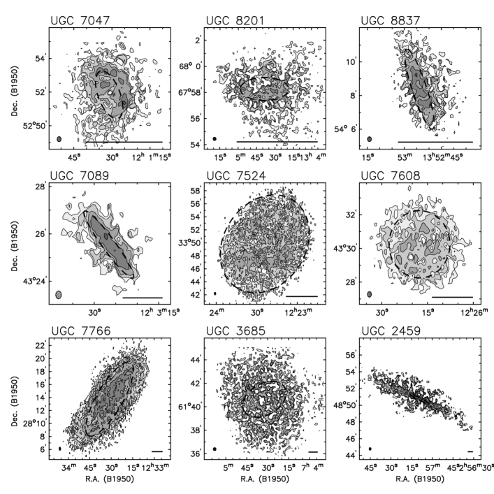
Figure 1: H i column density maps of six of the WHISP galaxies. The top three galaxies have total H i masses of $10^{8}\mbox{${\rm M}_{\odot}$}$, the middle three have $\mbox{$M_{\rm HI}$}\sim 10^{9}\mbox{${\rm M}_{\odot}$}$, and the bottom three have $\mbox{$M_{\rm HI}$}\sim 10^{10}\mbox{${\rm M}_{\odot}$}$. Contour levels are at column densities of $0.2$, $0.5$, $1$, $2$, $4$, $8$ and $16\times 10^{21}\,\mbox{$\rm cm^{-2}$}$, where the lowest contour corresponds to the DLA limit. The beam sizes are indicated in the lower left corners of each panel. The ellipses indicate the orientation parameters of the optical images of these galaxies and the extent corresponds to the diameter measured at the 25th $B$-magnitude isophote. The scale bar in the lower right corner corresponds to 5 kpc at the distance of the galaxies.

The sample from which WHISP candidates have been selected consists of galaxies in the Uppsala General Catalogue (UGC) of Galaxies (Nilson, 1973) that fit the following criteria: 1) $B$-band major axis diameter more extended than $1.2\arcmin$; 2) declination (B1950) north of $+20^{\circ}$; and 3) the 21-cm flux density averaged over the H i profile exceeds $100$ mJy. For observations after the year 2000 the flux density criterion was relaxed to also include galaxies with lower average flux densities. This enabled observation of a reasonably large number of galaxies of Hubble type S0 - Sb, which typically have lower H i fluxes than galaxies of Hubble type Sbc and later. For the analysis presented in this paper we made use of the data of 355 galaxies out of the total of 391 in the WHISP sample, which had been fully reduced at the time this analysis started. The distribution over Hubble type and optical luminosity for the 355 galaxies in our sample is given in table 1.

Table 1: Properties of the WHISP sample

	$L_{B}<L_{B}^{*}/20$	$L_{B}^{*}/20<L_{B}<L_{B}^{*}/5$	$L_{B}^{*}/5<L_{B}<L_{B}^{*}$	$L_{B}>L_{B}^{*}$	Total
E/S0	2	2	8	9	21
Sa/Sb	4	7	31	41	83
Sbc/Sc	7	14	37	52	110
Scd/Sd	19	15	17	4	55
Sm/Irr	43	31	7	5	86
Total	75	69	100	111	355

A total of about 4500 hours of observing time (more than one year of continuous data taking) was used over a period of 10 years to observe 391 galaxies. Of these, 281 were observed with the old WSRT system between 1992 and 1998. The remaining 110 galaxies were observed with the upgraded, more sensitive system between 2000 and 2002. The main difference between the two periods is the upgrade of the WSRT with cooled receivers on all telescopes and a greatly improved bandwidth and correlator capacity. In practice this means that the sensitivity of the observations made in 2000 and thereafter are a factor of $\sim 4$ better than before (e.g. a typical r.m.s. of 0.8 mJy/beam as compared to 3 mJy/beam). The velocity resolution for most galaxies is 5 km s^-1. The highly inclined galaxies in the sample with inclinations typically above $60^{\circ}$ have been observed at a lower velocity resolution of 20 km s^-1, while more face-on galaxies and galaxies with narrow single dish profiles ($\Delta v\leq 60\,\mbox{$\rm km\,s^{-1}$}$) have been observed with a velocity resolution of $2.5\,\mbox{$\rm km\,s^{-1}$}$.

The WSRT observations of the WHISP galaxies have been processed following a well described standard procedure consisting of a (u,v) data processing phase (data editing, calibration and Fourier transformation) using the native WSRT reduction package NewStar and an image processing phase (continuum subtraction, cleaning, determination of H i distributions and velocity fields using GIPSY. The resulting data cubes and images have been archived and a summary is displayed on the web at http://www.astro.rug.nl/$\sim$whisp. A precise description of the reduction procedures can also be found there.

For each observed galaxy the WHISP pipeline reduction recipe produces data cubes with an angular resolution of $\sim 12^{\prime\prime}\times 12^{\prime\prime}/\sin\delta$, $30^{\prime\prime}\times 30^{\prime\prime}$ and $60^{\prime\prime}\times 60^{\prime\prime}$. The maps with different resolutions are used to obtain some insight in the effect of spatial resolution on the measurement of H i cross sectional areas (see section 4.1). The median 3-$\sigma$ column density sensitivity limit of the highest resolution H i maps is $2.3\times 10^{20}~{}\mbox{$\rm cm^{-2}$}$. At the lower resolutions ($30^{\prime\prime}$ and $60^{\prime\prime}$) the column density sensitivities improve with factors of approximately 3.5 and 10, respectively. To illustrate the resolution of our data, we calculate the total number of beams over the optical area within the 25th magnitude isophote, and the number of beams over the area with an H i column density exceeding the DLA limit. These statistics are presented in Fig. 2. The median number of beams over the optical area is $\approx 40$, whereas the median number of beams over the H i area is $\approx 220$. We note that the total number of independent H i column density measurements above the DLA limit in our sample is $\approx 140,000$.

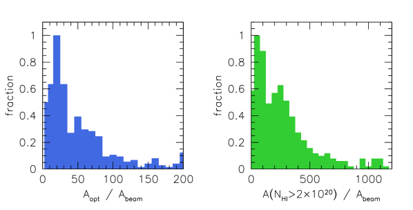
Figure 2: Left: Distribution of number of beams over the optical area within $D_{25}$. Right: Distribution of number of beams over the area with H i column density exceeding the DLA limit of $2\times 10^{20}\,\rm cm^{-2}$.

A possible concern about the selection of the WHISP sample is that the sample is based on the UGC, which implies that the parent sample from which the WHISP galaxies are chosen is optically selected. Since DLA systems are purely H i-selected, our $z=0$ comparison sample of galaxies should ideally also be H i-selected to guarantee that all possible optical selection biases are ruled out. However, Zwaan (2000) has shown that the properties of H i-selected galaxies are not different from those of optically selected galaxies if compared at the same luminosity. Specifically, he showed that the gas richness, optical surface brightness, and scale length of optically selected and H i-selected galaxies are indistinguishable if subsamples with similar median absolute magnitude are compared. Therefore, if the weighting of the sample is properly taken into account (using the luminosity function or H i mass function) no strong biases should be introduced by using optically selected galaxies. As will be discussed in section 4, we use morphological type-specific H i mass functions to calculate weights for individual galaxies, which will ensure that the morphological type distribution of our weighted sample at a given H i mass is similar to that of an H i-selected galaxy sample. Small differences in the optical properties of optically and H i-selected samples as a function of H i mass might remain, but given the findings of Zwaan (2000) and the fact that we apply type-specific weighting, these differences are unlikely to bias are results significantly. This is also illustrated by the fact that the value for the redshift number density $dN/dz$ that we derive in section 6 is consistent with what Ryan-Weber, Webster, & Staveley-Smith (2003); Ryan-Weber, Webster, & Staveley-Smith (2005a) find based on a smaller sample of H i-selected galaxies.

The field of view of the 21-cm WSRT observations is defined by the diameter of the individual dishes and is approximately $30^{\prime}$ across (at half power beam width). The WHISP data base contains many instances of multiple H i detections within one such field. We separated these multiple detections into individual galaxies if both H i detections could be identified with optically identifiable galaxies in the NASA/IPAC Extragalactic Database (NED). In most cases the multiple detections are known pairs or groups of galaxies. If a second H i detection in the field targeted on a UGC galaxy could not be associated with a catalogued galaxy, we did not separate this H i detection but treated it as a companion H i cloud to the known optical galaxy and therefore included it in the total cross section calculation, keeping information about the impact parameter at which the $N_{\rm HI}$ occurs.

All 21-cm maps of the resulting sample of galaxies were transformed to column density maps using the well-known equation

$$N_{\rm HI}=1.823\times 10^{18}\int T_{\rm B}(v)dv,$$ (1)

where $T_{\rm B}$ is the observed brightness temperature. This equation is valid for optically thin emission. For cold, high column density ($>10^{21}\,\mbox{$\rm cm^{-2}$}$) gas clouds, the optically thin approximation might break down, which would result in slightly underestimated H i column densities. This effect is probably only important for the very highest H i column densities, in the range where there are only very few DLA measurements. Therefore, it is unlikely to affect our comparison between DLAs and local galaxies. Furthermore, the measurement of total cross-sectional area above the DLA column density limit is not affected at all by H i optical depth effects.

3 Searches for low redshift DLA galaxies

The aim of this paper is to make a detailed comparison between the local galaxy population and local DLA galaxies. The difficulty in this comparison is that the number of identified DLA galaxies is very low, at any redshift. There are now approximately 600 DLA systems known in the Universe (Prochaska et al., 2005), only $\sim$ 50 of which are at $z<1.7$. This number is especially small at low redshifts, because the Ly-$\alpha$ line is only observable from the ground when it is redshifted to $z>1.7$. Furthermore, due to the expansion of the Universe, the expected number of absorbers along a line of sight decrease with decreasing redshift, which naturally leads to a scarcity of DLA systems at low $z$.

At high $z$ there is a substantial number of systems available, but attempts to directly image their host galaxies have generally been unsuccessful (see e.g., Colbert & Malkan, 2002; Møller et al., 2002; Prochaska et al., 2002). A few positive identifications do exist, mostly the result of HST imaging (Fynbo, Møller, & Warren, 1999; Warren et al., 2001; Kulkarni et al., 2000; Møller et al., 2002). Possibly the best data to date are available for three objects imaged with STIS by Møller et al. (2002). They found emission from three DLA galaxies with spectroscopic confirmation and concluded that the objects are consistent with being drawn from the population of Lyman-break galaxies.

Although the absolute number of DLAs at low $z$ is small, the success rate for finding their host galaxies is better for obvious reasons: the host galaxies are expected to be brighter and the separation on the sky between the bright QSO and the DLA galaxy is likely larger. The first systematic survey for low $z$ DLA host galaxies was performed by Le Brun et al. (1997), who obtained HST $R$ and $B$-band imaging of seven QSO fields with known DLAs. For most of their targets they found likely galaxies, the properties of which span a large range from LSB dwarfs to large spirals. Similar searches for single systems were done by Burbidge et al. (1996) and Petitjean et al. (1996). The DLA at $z=0.656$ in the sightline toward 3C336 was studied extensively by Steidel et al. (1997) and Bouché et al. (2001), but despite the deep HST imaging in the optical and H$\alpha$, no galaxy has been identified. All these studies lacked spectroscopic follow-up, so associations were purely based on the proximity of identified galaxies to the QSO sight line, which is not unique in many cases. Optical and infrared imaging combined with spectroscopic follow-up observations was first done by Turnshek et al. (2001), who successfully identified two galaxies at $z=0.091$ and $z=0.221$. Using a similar technique, Lacy et al. (2003) also identified two low $z$ DLA galaxies. Chen & Lanzetta (2003) demonstrated that it is possible to use photometric redshifts to determine the association of optically identified galaxies with DLAs, and applied this technique to six DLA systems. Finally, Rao et al. (2003) studied four DLA systems and were able to confirm two DLA galaxies based on spectroscopic confirmation, one using a photometric redshift, and one association was based on proximity to the QSO.

Two attempts have been made to measure directly the cold gas contents of low $z$ DLA systems by means of deep 21-cm emission line observations (Kanekar et al., 2001; Lane, Briggs, & Smette, 2000). The problem with these observations is that the 21-cm line is extremely weak so that with present technology surveys are limited to the very local ($z<0.2$) Universe. Both observations resulted in non-detections, which allowed the authors to put upper limits to the H i masses of approximately $\mbox{$M_{\rm HI}$}=2.3\times 10^{9}~{}\mbox{${\rm M}_{\odot}$}$, which is one third of the H i mass of an $L_{*}$ galaxy (Zwaan et al., 2003, 2005).

In addition to these surveys for low $z$ DLA galaxies, there are two cases of high column density absorption systems found in local galaxies. Miller, Knezek, & Bregman (1999) and Bowen, Tripp, & Jenkins (2001) study the absorption line systems seen in NGC 4203 and SBS 1543+593, at redshifts of $z=0.004$ and $z=0.009$, respectively. For these systems, the galaxy-QSO alignment was identified before the absorption was found and in one case (NGC 4203) Ly-$\alpha$ absorption has not been seen to date, but the structure and strength of observed metal lines resemble those of DLAs.

All together, including the $z\approx 0$ systems NGC 4203 and SBS 1543+593, there are now 20 DLA galaxies known at $z<1$. Table 2 summarises the properties of these galaxies. We have been fairly generous in assembling this table because not all listed galaxies have been spectroscopically confirmed. Also, some of the systems fall just below the classical DLA column density limit of $\log\mbox{$N_{\rm HI}$}=20.3$, but we decided to include these because our 21-cm emission line data is also sensitive below this limit. However, if in the remainder of this paper when we refer to “DLA column densities,” we restrict our analysis to $\log\mbox{$N_{\rm HI}$}>20.3$ and disregard the identified systems with lower column densities. Some systems in our compilation have been studied by several authors, in which case we choose the parameters from the most recent reference. The measurements of $L/L_{*}$ are mostly based on $B$-band data, but in some cases these data were not available in which cases we used $K$ or $R$-band. For the value of $L_{*}$ we adopted the recent measurement of $M_{B}^{*}-5\log h_{75}=-20.3$ from Norberg et al. (2002), $M_{R}^{*}-5\log h_{75}=-21.1$ from Lin et al. (1996), and $M_{K}^{*}-5\log h_{75}=-24.1$ from Cole et al. (2001). The morphological classifications are copied directly from the relevant references and are very heterogeneous in their degree of detail. Therefore, we note that the $L/L_{*}$ values and the listed types should be treated with caution and both parameters have large uncertainties. Our local DLA galaxy sample is defined to have redshifts $z<1$, which is of course a random choice. However, cutting the sample at lower redshift would result in too small a sample to make a meaningful comparison with our nearby galaxy statistics. The median redshift of the DLA galaxy sample is $<z>=0.5$. In the analysis we ignore any evolutionary effect in the redshift range $z=1$ to $z=0$. This assumption is justified by our finding in section 6, that the cross section times comoving space density of DLA systems is not evolving in this redshift range. However, an important caveat is that this lack of evolution in cross section puts no constraints on how gas is distributed in individual systems, but only on the total gas content averaged over the whole galaxy population. The mean properties of gas disks in galaxies might evolve since $z=1$. Given the fact that the cosmic star formation rate density drops by a factor $~{}8$ between $z=1$ and $z=0$ (e.g., Hopkins, 2004), it is possible that evolution of the neutral gas disks actually takes place as well. To study the H i mass evolution of galaxies deep observations with future instrument such as the Square Kilometer Array (SKA, Carilli & Rawlings, 2004) are required. At present no observational constraints exist. Apart from the evolution of the H i disks, the optical properties of DLA host galaxies could evolve between $z=1$ and $z=0$ as well. However, Chen & Lanzetta (2003) find that DLA galaxies do not show luminosity evolution between $z=1$ and $z=0$, although the constraints are limited by small number statistics.

Finally, one might be concerned about the process of choosing which galaxy to attribute to a certain absorber (see discussion in Chen & Lanzetta, 2003). In some cases more than one candidate is available, in which case the authors are forced to choose which one is the most likely absorber. The set of arguments on which this choice is based, varies between different studies. We note that this introduces some randomness in our compilation presented in Table 2.

Table 2: Properties of $z<1$ (sub-)DLA host galaxies.

QSO	$z_{\rm abs}$	log $N_{\rm HI}$	$b$	$L/L_{*}$	Morphology	Reference	Redshift1
		(cm-2)	(kpc)
Ton 1480	0.004	20.34	7.9	0.44	early type	a	spectro-z
HS 1543+5921	0.009	20.34	0.4	0.02	early type	b	spectro-z
Q0738+313	0.091	21.18	$<$3.1	0.08	LSB	c	no
PKS 0439-433	0.101	20.00	6.8	1.00	disk	d,g,k	spectro-z
Q0738+313	0.221	20.90	17.3	0.17	dwarf spiral	c,g	spectro-z
PKS 0952+179	0.239	21.32	$<$3.9	0.02	dwarf LSB	e	photo-z
PKS 1127-145	0.313	21.71	$<$5.6	0.16	Patchy irr LSB2	e,g,l	spectro-z
PKS 1229-021	0.395	20.75	6.6	0.17	Irr LSB	f	no
Q0809+483	0.437	20.80	8.3	2.80	giant Sbc	f,j,k	spectro-z
AO 0235+164	0.524	21.70	12.5	1.90	late-type spiral 2	g,m	spectro-z
B2 0827+243	0.525	20.30	29.5	1.04	disturbed spiral	e,g	spectro-z
PKS 1629+120	0.531	20.69	14.7	0.78	spiral	e,g	spectro-z
LBQS 0058+0155	0.613	20.08	7.5	0.60	spiral	h,k	spectro-z
Q1209+107	0.630	20.20	9.7	1.90	spiral	f	no
HE 1122-1649	0.681	20.45	23.5	0.58	compact	g	photo-z
Q1328+307	0.692	21.19	5.7	0.67	LSB	f	no
FBQS 1137+3907C	0.720	21.10	10.3	0.20	spiral?	i	spectro-z
FBQS 0051+0041A	0.740	20.40	22.4	0.80	spiral?	i	spectro-z
MC 1331+170	0.744	21.17	25.1	3.00	edge-on spiral	f	no
PKS 0454+039	0.860	20.69	5.5	0.60	compact	f,j	no

References: (a) Miller, Knezek, & Bregman (1999); (b) Bowen, Tripp, & Jenkins (2001); (c) Turnshek et al. (2001); (d) Petitjean et al. (1996); (e) Rao et al. (2003); (f) Le Brun et al. (1997); (g) Chen & Lanzetta (2003); (h) Pettini et al. (2000); (i) Lacy et al. (2003); (j) Colbert & Malkan (2002); (k) Chen, Kennicutt, & Rauch (2005); (l) Lane et al. (1998); (m) Burbidge et al. (1996)
¹ Indication of whether the redshift of the DLA galaxy has been confirmed by either spectroscopy or a photometric redshift measurement
² Probably arising in galaxy group

The conclusion from studying Table 2 is that the sample of low $z$ DLA galaxies spans a wide range in galaxy properties, ranging from inconspicuous LSB dwarfs to giant spirals and even early type galaxies. Obviously, it is not just the luminous, high surface brightness spiral galaxies that contribute to the H i cross section above the DLA threshold, although it is these galaxies that contribute most to the total comoving density $\Omega_{\rm HI}$.

4 Calculating the column density distribution function - $f(N_{\rm HI})$

In QSO absorption line studies, the column density distribution $f(N_{\rm HI})$ function is defined such that $f(\mbox{$N_{\rm HI}$})d\mbox{$N_{\rm HI}$}dX$ is the number of absorbers with column density between $N_{\rm HI}$ and $\mbox{$N_{\rm HI}$}+d\mbox{$N_{\rm HI}$}$ over an absorption distance interval $dX$. The analysis in this paper derives $f(N_{\rm HI})$ from the statistics of H i emission line distributions in the local galaxy population in order to predict the effectiveness of present day galaxies at accounting for the absorption line statistics. The parameter $dX$ assures that $f(\mbox{$N_{\rm HI}$})$ counts the number of absorbers per co-moving unit of length, but since $dX/dz=1$ at $z=0$, we can replace $dX$ with $dz$ in our calculation of $f(\mbox{$N_{\rm HI}$})$. The local $f(\mbox{$N_{\rm HI}$})$ can now be calculated from

$$f(\mbox{$N_{\rm HI}$})=\frac{c}{H_{0}}\frac{\sum_{i}\Phi({\bf x}_{i})w({\bf x}_{i})A_{i}(\log\mbox{$N_{\rm HI}$})}{\mbox{$N_{\rm HI}$}\,\ln 10\,\Delta\log\mbox{$N_{\rm HI}$}}.$$ (2)

Here, $\Phi({\bf x}_{i})$ is the space density of objects with property ${\bf x}_{i}$ equal to that of galaxy $i$. In reality, the parameter ${\bf x}$ could be the H i mass or the optical luminosity of the galaxies in the sample, so that $\Phi({\bf x})$ is the H i mass function or the optical luminosity function of galaxies in the local Universe. $A_{i}(\log\mbox{$N_{\rm HI}$}$) is the area function that describes for galaxy $i$ the area in $\rm Mpc^{2}$ corresponding to a column density in the range $\log\mbox{$N_{\rm HI}$}$ to $\log\mbox{$N_{\rm HI}$}+\Delta\log\mbox{$N_{\rm HI}$}$. In practice, this is simply calculated by summing for each galaxy the number of pixels in a certain $\log\mbox{$N_{\rm HI}$}$ range multiplied by the physical area of a pixel. The function $w({\bf x}_{i})$ is a weighting function that takes into account the varying number of galaxies across the full stretch of $\bf x$, and is calculated by taking the reciprocal of the number of galaxies in the range $\log{\bf x}-\Delta/2$ to $\log{\bf x}+\Delta/2$, where $\Delta$ is taken to be 0.3. The results are very insensitive to the exact value of $\Delta$. The summation sign denotes a summation over all galaxies in the sample. Finally, $c/H_{0}$ converts the number of systems per Mpc to that per unit redshift. Note that dependencies on $H_{0}$ disappear in the final evaluation of $f(\mbox{$N_{\rm HI}$})$.

The WHISP sample that is used in this analysis is somewhat biased toward early type galaxies (S0 to Sb) because these were specifically targeted for the projects described in van der Hulst, van Albada, & Sancisi (2001). If we were to apply a simple weighting scheme using a luminosity or H i mass function, early type galaxies would be given too much weight in the calculation of the $f(\mbox{$N_{\rm HI}$})$. To avoid this problem, we choose to apply type-specific H i mass functions as published by Zwaan et al. (2003). Morphological types are available in LEDA for all but 18 galaxies in the WHISP sample. We divide the WHISP sample into five subsets of galaxies: E-S0, Sa-Sb, Sbc-Sc, Scd-Sd, and Sm-Irr. Visual inspection of the unclassified galaxies learned that these were mostly dwarf irregular or small compact galaxies and hence we put these in the Sm/Irr subset. We note that the difference between the $f(\mbox{$N_{\rm HI}$})$ calculated using the weights based on one H i mass function for all WHISP galaxies and that based on type-specific weighting is very small.

Fig. 3 shows our measured column density distribution function $f(\mbox{$N_{\rm HI}$})$. We use a binning of $\log\mbox{$N_{\rm HI}$}=0.1\,\rm dex$. The error bars indicate $1\sigma$ uncertainties and include uncertainties in the H i mass function normalisation from Zwaan et al. (2003) as well as counting statistics of the WHISP sample. The open symbols indicate column densities below $\log\mbox{$N_{\rm HI}$}=19.8$, which we adopt as our sensitivity limit (see Section 4.1 for a discussion on this limit). Following Pei & Fall (1995), Storrie-Lombardi, Irwin, & McMahon (1996), Storrie-Lombardi & Wolfe (2000), and Péroux et al. (2003), we fit $f(\mbox{$N_{\rm HI}$})$ with a gamma distribution, analogous to the Schechter function, which is used for fitting luminosity functions and H i mass functions:

$$f(\mbox{$N_{\rm HI}$})=(f^{*}/\mbox{$N^{*}_{\rm HI}$})(\mbox{$N_{\rm HI}$}/\mbox{$N^{*}_{\rm HI}$})^{-\beta}e^{-\mbox{$N_{\rm HI}$}/\mbox{$N^{*}_{\rm HI}$}}.$$ (3)

This gives an excellent fit to our data with parameters: $\beta=1.24$, $\log\mbox{$N^{*}_{\rm HI}$}=21.2\,\mbox{$\rm cm^{-2}$}$, and $f^{*}=0.0193$ if we use all data points above $\log\mbox{$N_{\rm HI}$}>19.8$. The parametric $f(\mbox{$N_{\rm HI}$})$ is shown as a solid line in Fig. 3. If we restrict the fit to column densities above the DLA limit, we find $\beta=1.52$, $\log\mbox{$N^{*}_{\rm HI}$}=21.3\,\mbox{$\rm cm^{-2}$}$, and $f^{*}=0.0137$, which is shown by the dotted line. We note that there is no physical motivation for fitting the $f(\mbox{$N_{\rm HI}$})$ with a gamma distribution other than that it provides a reasonable fit. Neither is there a physical reason to fit $f(\mbox{$N_{\rm HI}$})$ with a power law, which is traditionally done (e.g., Tytler, 1987). However, the good gamma distribution fit demonstrates that at high H i column densities ($\log\mbox{$N_{\rm HI}$}>21$), the $f(\mbox{$N_{\rm HI}$})$ deviates strongly from a traditional single power-law fit. This is consistent with the form of the cut-off identified by Péroux et al. (2003) based on a large sample of DLAs and sub-DLAs.

Figure 3: The H i column density distribution function at $z=0$ from 21-cm emission line observations. Error bars include uncertainties in the H i mass function as well as counting statistics and indicate $1\sigma$ uncertainties. Open symbols correspond to measurements below our sensitivity limit. The solid line is a gamma distribution fit (see Eq. 3) to all points above $\log\mbox{$N_{\rm HI}$}>19.8$, the dotted line is the same but restricted to $\log\mbox{$N_{\rm HI}$}>20.3$.

The total H i mass density can be calculated by integrating over the column density distribution function. When using the parametrised gamma distribution, it can be easily seen that the H i mass density can be calculated as

$$\rho_{\rm HI}=\Gamma(2-\beta)f^{*}\mbox{$N^{*}_{\rm HI}$}\,m_{\rm H}\,H_{0}/c,$$

where $m_{\rm H}$ is the mass of the hydrogen atom and $\Gamma$ is the Euler gamma-function. Using the best-fit parameters of our gamma distribution fit to $\log\mbox{$N_{\rm HI}$}>19.8$, we find $\rho_{\rm HI}=6.8\times 10^{7}\mbox{${\rm M}_{\odot}$}\rm Mpc^{-3}$, in excellent agreement with Zwaan et al. (2003). This may not come as a surprise, since we used the H i mass functions from that paper to calibrate $f(N_{\rm HI})$. Nonetheless, the result of this calculation is a good consistency check and assures that the normalisation of our $f(\mbox{$N_{\rm HI}$})$ is correct (see also Rao & Briggs, 1993).

There are a few interesting features in Fig. 3. First, our measured points begin to deviate from the power law end of the gamma distribution fit at column densities $\log\mbox{$N_{\rm HI}$}<19.8$. The first obvious explanation for this is that in this range of $N_{\rm HI}$ we start to loose sensitivity in the 21-cm maps. There might also be a more physical origin of this effect, which is the expected ionisation of the outer H i disks of galaxies by the metagalactic UV-background below $\log\mbox{$N_{\rm HI}$}\approx 19.5$ (Corbelli & Salpeter, 1993; Maloney, 1993). Corbelli & Bandiera (2002) argue that if $f(N_{\rm HI})$ is corrected to include H ii, it would follow a power-law down to $\mbox{$N_{\rm HI}$}=10^{17}~{}\mbox{$\rm cm^{-2}$}$. Our 21-cm maps lack the sensitivity to study this effect in detail. At the high $N_{\rm HI}$ end in Fig. 3, the $f(N_{\rm HI})$ drops off exponentially, which is faster than $\mbox{$N_{\rm HI}$}^{-3}$ above $\log\mbox{$N_{\rm HI}$}=21.6$. A fall-off of $\mbox{$N_{\rm HI}$}^{-3}$ is theoretically expected for randomly oriented gas disk, irrespective of their radial $N_{\rm HI}$ distribution (see Milgrom, 1988; Fall & Pei, 1993; Zwaan, Verheijen, & Briggs, 1999). Three independent effects can cause deviation of the $\mbox{$N_{\rm HI}$}^{-3}$ expectation: 1) beam smearing in the 21-cm maps can smooth out the very highest column densities; 2) galaxies are not infinitely thin (this is assumed in the $f(N_{\rm HI})$ calculation of randomly oriented disks); and 3) the H i gas is not optically thin at the highest column densities. In the remainder of this paper, our possible biases at the extreme edges of $f(\mbox{$N_{\rm HI}$})$ are not important because we only compare our data with the absorption line data in the intermediate $N_{\rm HI}$ range. Furthermore, the cosmological H i mass density is also dominated by the intermediate $N_{\rm HI}$ values, as will become clear in section 5.

4.1 The effect of spatial resolution on $f(N_{\rm HI})$

One concern when comparing column densities measured from 21-cm maps with those measured from absorption line systems is the large difference in spatial resolution. The median distance of the WHISP sample is 20 Mpc, implying that for the highest resolution maps the synthesised beam corresponds to $\approx 1.3$ kpc. This is almost $10^{5}$ times greater than the diameter of the optical emission region of a QSO ($\leq 0.03$ pc, e.g. Wyithe, Agol, & Fluke 2002), the area probed by DLA column density measurements.

Despite this disparity in resolution, 21-cm emission and Lyman $\alpha$ absorption measurements generally seem to be in agreement. Dickey & Lockman (1990) noted a consistency between Lyman $\alpha$ absorption measurements towards high latitude stars and 21-cm emission measurement in the Galaxy. There is only one example where a column density from both 21-cm emission and DLA absorption has been measured of the same source. The DLA galaxy SBS 1543+593 has Lyman $\alpha$ absorption measured at $2.2\times 10^{20}\,\mbox{$\rm cm^{-2}$}$ (Bowen, Tripp, & Jenkins, 2001), whereas the 21-cm emission at the position of the background QSO is measured to be $5\times 10^{20}\,\mbox{$\rm cm^{-2}$}$ (Chengalur & Kanekar, 2002).

An alternative method to test the effect of resolution is to spatially smooth high resolution 21-cm maps and measure the resulting column densities and $f(N_{\rm HI})$. Ryan-Weber, Staveley-Smith, & Webster (2005b) used a high resolution 21-cm data cube of the Large Magellanic Cloud and convolved it with circular 2-dimensional Gaussians of various widths in the spatial plane. The $N_{\rm HI}$ distribution was then re-measured and $f(N_{\rm HI})$ was re-calculated, based on the new, low resolution column densities. Lowering the resolution was found to have a truncating effect on the $N_{\rm HI}$ distribution, generally decreasing the occurrence of the highest column densities.

For our set of WSRT maps, we can test the effect of lowering the spatial resolution. This is shown in Fig 4, where we present the $f(N_{\rm HI})$ distribution derived from the $30^{\prime\prime}$ and $60^{\prime\prime}$ maps, along with that from the original resolution maps. It can be seen that going to lower resolution, the highest column densities are smoothed away and this flux appears again as lower column densities. Effectively, this causes a ‘tilt’ of $f(N_{\rm HI})$. From this sample it is impossible to estimate if this tilting would continue if even higher resolution maps would be used. However, for our comparison with DLA data the effect of resolution is probably unimportant because the effects are minimal in the intermediate $N_{\rm HI}$ range where we make the comparison.

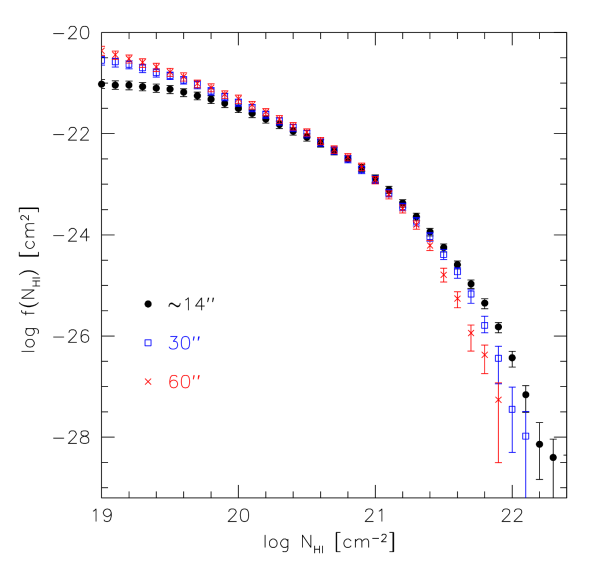
Figure 4: The effect of spatial resolution of the 21-cm line observations on the H i column density distribution function at $z=0$. Filled circles correspond to the highest resolution, which is approximately $14^{\prime\prime}$, open squares and crosses are for the spatially smoothed data, to resolutions of $30^{\prime\prime}$ and $60^{\prime\prime}$, respectively.

The redshift number density, $dN/dz$ (see section 6) is also only minimally affected by resolution. The LMC study by Ryan-Weber, Staveley-Smith, & Webster (2005b) showed that $dN/dz$ (at a limit of $\log\mbox{$N_{\rm HI}$}=20.3$) increases on the order of 10 per cent when the spatial resolution is changed from 15 pc to 1.3 kpc, the typical resolution of the WHISP sample. A 10 per cent change in the measured $dN/dz$ for the WHISP sample is well within the errors quoted in section 6.

Finally, we comment on our adopted sensitivity limit of $\log\mbox{$N_{\rm HI}$}=19.8$ for the column density distribution function. In Section 2 we quoted a formal 3$\sigma$ sensitivity limit of $\log\mbox{$N_{\rm HI}$}=20.3$ for the high resolution maps, which implies that below this limit we might start to underestimate $f(N_{\rm HI})$. However, Fig. 4 shows that $f(N_{\rm HI})$ based on lower resolution data is marginally higher in the range $19.8<\log\mbox{$N_{\rm HI}$}<20.3$, and only significantly deviates from the high resolution curve for $\log\mbox{$N_{\rm HI}$}<19.8$. As explained above, the higher $f(N_{\rm HI})$ values for lower resolution data are not only the result of these data having lower sensitivity limits and thus picking up lower column density H i, but also because small regions of high $N_{\rm HI}$ gas are smoothed away and appear again as lower column densities. This also explains why small differences between $f(N_{\rm HI})$ based on the different resolution data already become apparent above $\log\mbox{$N_{\rm HI}$}=20.3$. Therefore, if we were to construct a “hybrid” $f(N_{\rm HI})$ using high $N_{\rm HI}$ results from high resolution data and low $N_{\rm HI}$ from low resolution data, we would double-count some of the H i atoms. We choose to simply adopt a sensitivity limit of $\log\mbox{$N_{\rm HI}$}=19.8$, and note that the low end ($\log\mbox{$N_{\rm HI}$}<20.3$) of $f(N_{\rm HI})$ might be slightly underestimated, but by not more than 20 per cent. This does not influence any of our conclusions presented in this paper.

5 Comparison of $f(N_{\rm HI})$ with high $z$ data

In Fig. 5 we reproduce the $f(N_{\rm HI})$ measurements from our analysis of 21-cm maps and compare these with data at higher redshifts from Péroux et al. (2005), Rao et al. (2005) and Prochaska et al. (2005). The Péroux et al. (2005) measurements of $f(N_{\rm HI})$ below the DLA limit are the result of their new UVES survey for “sub-DLAs”. We choose here to only plot the points for $\log\mbox{$N_{\rm HI}$}>19.8$, which roughly corresponds to our sensitivity cut-off. Their higher column density points stem from the combined data of Storrie-Lombardi, Irwin, & McMahon (1996), Storrie-Lombardi & Wolfe (2000), and Péroux et al. (2001), together based on $\approx 100$ $z>4$ quasars. The Prochaska et al. (2005) data are from an automatic search for $z>2.2$ DLA systems in SDSS-DR3 and also include the results from previous DLA surveys. We represent their results by both a gamma distribution fit and a double power-law fit to the whole data set in the redshift range $2.2<z<5.5$. The intermediate redshift points from Rao et al. (2005) are based on Mg ii-selected DLA systems. All calculations are based on a $\Omega_{\rm m}=0.3$, $\Omega_{\Lambda}=0.7$ cosmology. The surprising result from this figure is that there appears to be only very mild evolution in the intersection cross section of H i from redshift $z\sim 5$ to the present. This is a conclusion in stark contrast to earlier works that claimed strong evolution in the DLA cross section (e.g., Wolfe et al. , 1986; Lanzetta et al., 1991). We will come back to this weak evolution in section 6 in which we discuss the redshift number density.

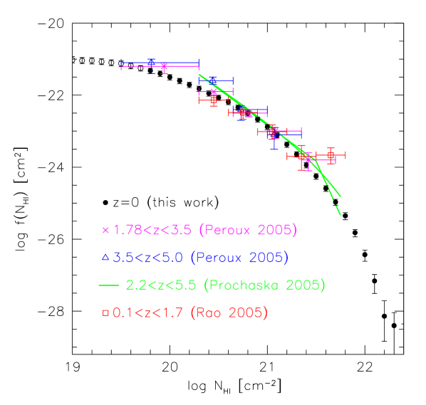
Figure 5: Comparison between the H i column density distribution function at $z=0$ and higher redshifts. The solid points are from our 21-cm emission line observations and are the same as in Fig. 3. The higher redshift points are from Péroux et al. (2005) and Rao et al. (2005). Horizontal errorbars indicate the bin sizes. The curves show the gamma distribution and double power-law fits to the SDSS-DR3 results from Prochaska et al. (2005) and cover a redshift range of $2.2<z<5.5$. All results based on a $\Omega_{\rm m}=0.3$ and $\Omega_{\Lambda}=0.7$ cosmology.

In Fig. 6 we plot the contribution of systems with different column densities to the integral H i mass density $\rho_{\rm HI}$. At $z=0$ it is clear that systems with column densities $\mbox{$N_{\rm HI}$}\sim 10^{21}\,\mbox{$\rm cm^{-2}$}$ dominate the H i mass density. At higher redshifts ($z>1.7$), the uncertainties are much larger, but also there it appears that $\mbox{$N_{\rm HI}$}\sim 10^{21}\,\mbox{$\rm cm^{-2}$}$ systems contribute most, although the Prochaska et al. (2005) data suggest that column densities between $\log\mbox{$N_{\rm HI}$}=20.3$ and $21.3$ contribute almost evenly. Any possible differences between the results at various redshifts are much more pronounced in Fig. 6 than in Fig. 5 because the vertical scale is stretched from nine decades to only four decades. The one point that clearly deviates is the highest $N_{\rm HI}$ point from Rao et al. (2005) at $\log\mbox{$N_{\rm HI}$}=21.65$. This elevated interception rate of high $N_{\rm HI}$ Mg ii-selected intermediate redshift DLAs is present in both redshift bins that Rao et al. (2005) distinguish ($0.1<z<0.9$ and $0.9<z<1.7$), and is also reported in their earlier work (Rao & Turnshek, 2000). Fig. 6 very clearly demonstrates that this point dominates the $\Omega_{\rm HI}$ measurement at intermediate redshifts. It is therefore important to understand whether the Mg ii-based results really indicate that high column densities ($\log\mbox{$N_{\rm HI}$}\sim 21.65$) are rare at high redshift, then indeed become more abundant at intermediate redshifts ($0.1<z<1.7$) and subsequently evolve to the scarce numbers at $z=0$. Alternatively, the high $f(N_{\rm HI})$ point might be a result of yet unidentified selection effects introduced by the Mg ii-selection, although presently there are no indications that support this (Péroux et al., 2004; Rao et al., 2005).

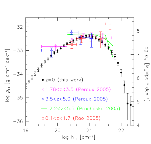
Figure 6: The H i mass density contained in systems of different column density per decade of $N_{\rm HI}$. Solid circles are for $z=0$ and are from our data, other symbols are for higher redshifts and are derived from Péroux et al. (2005) and Rao et al. (2005). The curves are the converted fits to the SDDS-DR3 results from Prochaska et al. (2005).

To further investigate the relative contribution of different column densities to the H i mass density, we plot in Fig. 7 the cumulative H i mass density as a function of column density. The solid curve is based on our measured $f(N_{\rm HI})$ points, not on the gamma distribution fit to the data. From this curve alone, we would conclude that at $z=0$ the fractional mass in systems with $\log\mbox{$N_{\rm HI}$}>20.3$ (classical DLAs) is 86 per cent. However, the contribution of gas with column densities below our sensitivity limit of approximately $\log\mbox{$N_{\rm HI}$}=19.8$ is very uncertain. Unfortunately, only selective regions have been imaged to low column density limits, but no large scale 21-cm emission line surveys that reach sensitivities below $\log\mbox{$N_{\rm HI}$}=19.8$ are available yet. For example, the M31 environment has been imaged with the GBT and the WSRT at resolutions between 50 pc and 11 kpc (Braun & Thilker, 2004, and references therein), covering the column density range $17<\log\mbox{$N_{\rm HI}$}<22$. However, the H i emission in this region is mostly due to discrete High Velocity Clouds (HVCs) physically associated to M31. These surveys may not be representative of all low column density H i gas at $z=0$, and do not provide good constraints on the shape of $f(N_{\rm HI})$. To obtain a rough estimate of the contribution of gas below our sensitivity limit, we extrapolate our measured $f(N_{\rm HI})$ below $\log\mbox{$N_{\rm HI}$}=19.8$ with $\mbox{$f(N_{\rm HI})$}\propto\mbox{$N_{\rm HI}$}^{-1.5}$ (per e.g., Tytler, 1987) and find that the fractional mass in systems with $\log\mbox{$N_{\rm HI}$}>20.3$ is $\approx 81$ per cent, and hence only $\approx 19$ per cent of the H i atoms in the local UniverUniverse are in sub-DLA column densities. For illustrative purposes, we also show as a shaded area the cumulative distribution functions based on the gamma distribution fits to $f(N_{\rm HI})$ as presented in Figure 3. Here, the fit to $\log\mbox{$N_{\rm HI}$}>19.8$ corresponds to the upper boundary and the fit to $\log\mbox{$N_{\rm HI}$}>20.3$ to the lower boundary to this area. Obviously, simply extrapolating the gamma distribution fits to $f(N_{\rm HI})$ below the DLA limit results in a severe overestimation of the number of H i atoms in sub-DLA systems.

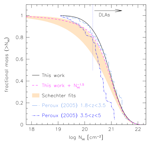
Figure 7: Cumulative H i mass distribution in systems with column density $>\mbox{$N_{\rm HI}$}$. The solid line is based on our data alone, the dashed line includes a correction for H i gas with column densities below our sensitivity limit and indicates that $\approx 81$ per cent of the integral mass in H i is in classical damped systems with $\log\mbox{$N_{\rm HI}$}>20.3\,\rm cm^{-2}$. The shaded area indicates the distribution based on the gamma distribution fits to our $f(N_{\rm HI})$ (Figure 3), where the lower boundary corresponds to the fit to $\log\mbox{$N_{\rm HI}$}>20.3$ and the upper boundary to the fit to $\log\mbox{$N_{\rm HI}$}>19.8$. The long-dashed and dash-dotted lines are from Péroux et al. (2005) and are for redshift ranges $1.8<z<3.5$ and $z>3.5$, respectively.

The higher redshift curves are based on the data of Péroux et al. (2005). With their new column density measurements of individual sub-DLAs, these authors improved the earlier estimates of $f(N_{\rm HI})$ presented in Péroux et al. (2003) and now show that the fractional contribution of sub-DLAs to $\Omega_{\rm HI}$ is approximately 20 per cent at all redshifts $z>1.8$. These curves also indicate that at high redshifts the highest column densities are relatively rarer, as can also be seen in Figure 5. Prochaska et al. (2005) estimate the fractional contribution of sub-DLA systems to the integral mass density by combining their measured $f(N_{\rm HI})$ with the redshift number density of sub-DLAs from Péroux et al. (2001). They conclude that the sub-DLAs (or super-LLSs in their terminology) contribute between 20 and 50 per cent over the redshift range 2.2 to 5.5, but emphasise that their single power-law fit to $f(N_{\rm HI})$ might even underestimate this fraction. Obviously, the importance of sub-DLA systems at high redshift remains a topic needing further clarification in the future.

The fact that from our high resolution 21-cm maps we find that $\approx 81$ per cent of the H i mass density at $z=0$ is in column densities above the DLA limit, implies that $\Omega_{\rm HI}$ measurements from blind 21-cm surveys overestimate $\Omega_{\rm DLA}(z=0)$ by only $\approx 23$ per cent. When comparing measurements of the atomic gas mass density at high and low redshifts, it is important that the $z=0$ value be corrected with a factor 0.81 when compared to measurements from DLAs. On the other hand, when at higher redshift the sub-DLA contribution is taken into account (e.g., Péroux et al., 2005), no correction of the $z=0$ value is required. We refer to Prochaska et al. (2005) for various definitions of $\Omega_{\rm gas}$ and their recommended usage.

6 The redshift number density at $\mbox{$z$}=0$

The redshift number density $dN/dz$ for column densities larger than $N_{\rm HI}$ can be calculated from the $z=0$ $f(N_{\rm HI})$ distribution by summing over all column densities larger than $N_{\rm HI}$:

$$dN/dz = \int_{N^{\prime}_{\rm HI}>N_{\rm HI}}f(N^{\prime}_{\rm HI})\,d{N^{\prime}_{\rm HI}}$$ (4)

$$= \frac{c}{H_{0}}\sum_{N^{\prime}_{\rm HI}>N_{\rm HI}}\frac{\sum_{i}\Phi({\bf x}_{i})w({\bf x}_{i})A_{i}(\log N^{\prime}_{\rm HI})}{\Delta\log N^{\prime}_{\rm HI}},$$ (5)

where definitions of $\Phi$, $w$, and $A_{i}$ are equal to those in section 4. In Fig. 8 we show $dN/dz$ as a function of $N_{\rm HI}$. For column densities in excess of the DLA limit of $\log\mbox{$N_{\rm HI}$}=20.3$ we find $dN/dz=0.045\pm 0.006$, where the $1\sigma$ uncertainty is dominated by the uncertainty in the parameters of the H i mass function that is used to calibrate $f(N_{\rm HI})$. For larger column densities $dN/dz$ drops rapidly, systems with $\log\mbox{$N_{\rm HI}$}>21$ contribute only 20 per cent to the total DLA cross section. Our measurement of $dN/dz$ translates into a mean cross section density of $<n\sigma>=(1.13\pm 0.15)\times 10^{-5}\,\rm Mpc^{-1}$, or to a mean free path between absorbers of $l=<n\sigma>^{-1}=88\pm 12\,\rm Gpc$.

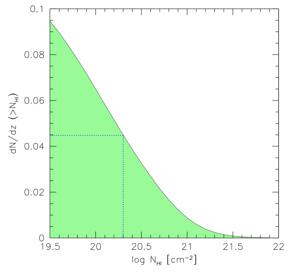
Figure 8: Integral redshift number density $dN/dz$ as a function of H i column density cut-off. For $\log\mbox{$N_{\rm HI}$}>20.3\,\rm cm^{-2}$ we find $dN/dz=0.045$, dropping rapidly for higher column densities.

The value of $dN/dz(z=0)=0.045$ agrees very well with our previous measurement of $dN/dz=0.042\pm 0.015$, based on a much smaller sample of galaxies (Zwaan, Briggs, & Verheijen, 2002). Rosenberg & Schneider (2003) used H i-selected galaxies to find $dN/dz=0.053\pm 0.013$, also in good agreement with our value. Their slightly higher value is probably the result of the steeper H i mass function slope that these authors use to calibrate their $f(N_{\rm HI})$. Ryan-Weber, Webster, & Staveley-Smith (2003) also used a sample of H i-selected galaxies observed with the ATCA and applied the same HI mass function normalisation as in the present analysis, to find $dN/dz=0.046^{+0.03}_{-0.02}$ (see also Ryan-Weber, Webster, & Staveley-Smith, 2005a). An earlier calculation by Rao & Briggs (1993) resulted in a much lower value of $dN/dz=0.015$. This discrepancy arises partly because these authors limited their analysis to large, optically bright galaxies, whereas the newer values take into account dwarf and low surface brightness (LSB) galaxies, and partly because their calculation is based on the Gaussian luminosity function from Tammann (1985), which has a lower normalisation than the most recent H i mass function measurements.

It has been noted before that the area of the H i disk of galaxies above the DLA limit correlates very tightly to the H i mass (e.g., Broeils, 1992; Rosenberg & Schneider, 2003). We can make use of this correlation to obtain a alternative measurement of $dN/dz$. Suppose that the projected H i area $A$ correlates with $M_{\rm HI}$ as $A\propto\beta\mbox{$M_{\rm HI}$}$, and $A^{*}$ is the projected area of an $\mbox{$M_{\rm HI}$}^{*}$ galaxy, then

$$dN/dz = \frac{c}{H_{0}}\int\theta(\mbox{$M_{\rm HI}$})A(\mbox{$M_{\rm HI}$})d\mbox{$M_{\rm HI}$}$$ (6)

$$= \frac{c}{H_{0}}\,A^{*}\theta^{*}\Gamma(1+\alpha+\beta),$$ (7)

where $\theta*$ and $\alpha$ are the normalisation and the low-mass power-law slope of the H i mass function, respectively. For our WHISP sample we find that $A^{*}=992\,\rm kpc^{2}$. Using this value, the Zwaan et al. (2003) H i mass function parameters ($\alpha=-1.30$ and $\theta^{*}=0.0086\,{\rm Mpc}^{-3}$), and $\beta=1$, we find that $dN/dz=0.044$. Quite surprisingly, this simplistic approach yields a result very close to our measurement of $dN/dz=0.045$ based on a much more detailed analysis.

6.1 Evolution of $dN/dz$

We now have a robust measurement of the redshift number density at $z=0$. How does this value compare to DLA measurements at higher redshifts? In Fig. 9 we show the combined results of high and low redshift $dN/dz$ measurements from different surveys. At $z=0$, we plot our points as well as those from Ryan-Weber, Webster, & Staveley-Smith (2003); Ryan-Weber, Webster, & Staveley-Smith (2005a) and Rosenberg & Schneider (2003). All these local values are based on analyses of H i 21-cm maps of galaxies, have small error bars and are consistent with each other. The points at $z\approx 0.6$ and $z\approx 1.2$ are from Rao et al. (2005) based on their $z<1.65$ HST survey of Mg ii selected systems from the SDSS-EDR. Their total sample of $z<1.65$ DLAs is now 41, which is a considerable improvement over the original sample of 16 DLAs presented in Rao & Turnshek (2000). The underlying assumption that the incidence of DLA systems can be derived from Mg ii surveys relies on the empirical fact that all DLA systems show Mg ii absorption, whereas the reverse is not true. The known incidence of Mg ii systems can therefore be used to bootstrap the DLA statistics. A similar technique was used by Churchill (2001) , who found $dN/dz=0.08^{+0.09}_{-0.05}$ at a median redshift of $z=0.05$. This number is based on HST data on four Mg ii absorbers. The high redshift points from Prochaska et al. (2005) are the result of an automatic search for $z>2.2$ DLA systems in SDSS-DR3 and also include the results from previous DLA surveys as summarised in Storrie-Lombardi & Wolfe (2000) and Péroux et al. (2003).

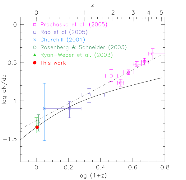
Figure 9: Number density of DLAs per unit redshift as function of redshift. All points at $z>0.1$ are from UV and optical surveys for DLA systems or MgII systems (see text). The points at $z\sim 0$ are from techniques similar to that presented in this work. The dashed line shows the best fit to $dN/dz$ from Storrie-Lombardi & Wolfe (2000). The solid line represents “no evolution in the product of cross section and co-moving space density” for a cosmology with $\Omega_{\rm m}=0.3$ and $\Omega_{\Lambda}=0.7$. This line is scaled vertically so as to fit our $z=0$ point.

Also shown in Fig. 9 by a dashed line is the fit $dN/dz=0.055(1+z)^{1.11}$ from Storrie-Lombardi & Wolfe (2000), which agrees reasonably well with the $z=0$ value. It is often quoted in the literature that this fit indicates “no intrinsic evolution in the product of space density and cross-section” of damped absorbers, which is another way of saying that the number of systems per co-moving unit of length does not evolve. This statement is based on the fact that for a $q_{0}=0$ Universe, $dX/dz=1+z\approx(1+z)^{1.11}$. However, for a modern non-zero $\Lambda$ Universe, $dX/dz$ is given by

$$\frac{dX}{dz}=\frac{(1+z)^{2}}{\sqrt{\Omega_{\rm M}(1+z)^{3}-(\Omega_{\rm M}+\Omega_{\Lambda}-1)(1+z)^{2}+\Omega_{\Lambda}}},$$ (8)

which starts to deviate significantly from the $q_{0}=0$ prediction for $z>1$. For no evolution in the number of systems per co-moving unit of length, we expect

$$\frac{dN}{dz}=\left(\frac{dN}{dz}\right)_{z=0}\frac{dX}{dz}.$$ (9)

The solid line in Fig. 9 represents this run of $dN/dz$ as function of $z$ for an $\Omega_{\rm m}=0.3$ and $\Omega_{\Lambda}=0.7$ Universe. We normalise this line to our $dN/dz(z=0)=0.045$ measurement. With respect to this $\Omega_{\rm m}=0.3$, $\Omega_{\Lambda}=0.7$ prediction, there is only weak evolution in the comoving incidence rate from $z\sim 4$ to the present time. Between $z\sim 1.5$ and $z=0$ there is no evidence for evolution at all, between $z\sim 4$ and $z=0$, the evolution in the comoving incidence rate is approximately a factor 2.

This conclusion contrasts with previous claims that the local galaxy population cannot explain the DLA incidence rate. For example, estimates of the cross section to DLA absorption in local galaxy disks by Wolfe et al. (1986) and Lanzetta et al. (1991) indicated that there should be evolution of at least a factor of 2 to 4 (depending on the value of $q_{0}$). Likewise, the analysis of Rao & Briggs (1993) pointed toward strong evolution in the incidence rate since $z=2.5$. Part of the reason for our conclusion being different from older works, is the change in cosmological parameters. For no evolution in the comoving number density in a $q_{0}=0.5$ cosmology, the allowed change in $dN/dz$ is much smaller than that for a modern $\Omega_{\rm m}=0.3$, $\Omega_{\Lambda}=0.7$ cosmology. The other reason is that the galaxy luminosity functions that were used for older $dN/dz$ calculations had a lower normalisation than the more recent estimates from large scale optical and 21-cm surveys.

We emphasise that the normalisation of $f(N_{\rm HI})$ and hence of $dN/dz$ is completely independent of the WHISP galaxy sample, but instead depends only on the H i mass functions derived from HIPASS. This is a large scale blind 21-cm emission line survey covering the whole southern hemisphere and the redshift range $z=0$ to $z=0.04$. Most of the weight to the normalisation of the H i mass function comes from galaxies around $z=0.01$. Optical and infrared surveys have shown that a large angular area around the southern Galactic pole is underdense by $\approx 25$ per cent extending out to $z=0.1$ (Frith et al., 2003; Busswell et al., 2004). This area occupies approximately one third of the HIPASS sky coverage, but it is not clear whether the underdensity extends to even larger regions in the southern hemisphere. In any case, our measured $f(N_{\rm HI})$ and $dN/dz$ might be underestimated by up to 25 per cent due to this local galaxy deficiency. This implies that the evolution in the comoving incidence rate is perhaps even slightly weaker than portrayed in Fig. 9.

The lack of evolution in the comoving incidence rate since redshift $z\sim 1.5$ implies that the average H i cross section above the DLA limit has not changed significantly over half the age of the Universe. At present, it is difficult to ascertain whether this should be interpreted as no evolution in the DLA population – meaning no change in the space density and size of DLA absorbing systems – or as a combined effect where an evolving space density is compensated by a change in mean absorber size.

7 Expected properties of low-redshift DLA host galaxies

In this section we calculate the probability distribution functions of the expected properties of galaxies responsible for high column density H i absorption at $z=0$. To this end, we define a quantity $\mathcal{N}$ as the ‘volume density of cross sectional area’ for different column density cut-offs. $\mathcal{N}$ is calculated as

$$\mathcal{N}({\bf y})=\int\Sigma({\bf y},{\bf x})\Phi({\bf x})d{\bf x},$$ (10)

where $\Sigma({\bf y},{\bf x})$ is the cross-sectional area of H i in Mpc² above a certain column density cut-off as a function of galaxy properties ${\bf x}$ and ${\bf y}$, and $\Phi({\bf x})$ is the space density of galaxies in $\rm Mpc^{-3}$ as a function of ${\bf x}$. Similarly to the calculation of $f(\mbox{$N_{\rm HI}$})$, the parameter ${\bf x}$ has elements $M_{\rm HI}$ and $L$, such that $\Phi$ is again the H i mass function or the optical luminosity function that is used to calculate real space densities. The vector ${\bf y}$ could be any galaxy property, such as optical surface brightness or morphological type. For example, if ${\bf x}=\mbox{$M_{\rm HI}$}$ and ${\bf y}=\mu$, we calculate $\mathcal{N}(\mu)$, the volume density of cross-sectional area as function of surface brightness $\mu$, using the H i mass function to calculate space densities. In the remainder of this paper we will use ${\bf x}=\mbox{$M_{\rm HI}$}$, so that the H i mass function is used for calibration. We find that the conclusions would not change significantly if we were to use the optical luminosity function instead.

Another way of looking at $\mathcal{N}$ is that it defines the number of systems above a certain column density limit that would be encountered along a random 1 Mpc path through the $z=0$ Universe. Put differently, $\mathcal{N}$ can be written as $dN/dz\times H_{0}/c$, where $dN/dz$, the number of systems per unit redshift, is a familiar quantity in QSO absorption line studies. The run of $\mathcal{N}$ as a function of galaxy property x represents the probability distribution of x of galaxies responsible for absorption above a certain column density.

In the following, we present this probability distribution for four different column density limits, $\log\mbox{$N_{\rm HI}$}>19.8$, $>20.3$, $>20.8$, and $>21.3$. The distribution for $\log\mbox{$N_{\rm HI}$}=20.3$, which is the classical DLA limit, is always shown as a thick line. In table 3 we tabulate the relative contributions of galaxies of different luminosities and H i masses to the total DLA cross section. In table 4 the mean and median properties of expected DLA host galaxies are summarized.

7.1 Luminosities

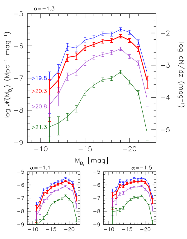
Figure 10: The expected distribution of absolute $B$-band magnitudes of high column density H i absorbing systems. The lines plus errorbars show the product of cross sectional area and space density, which translates to the number of expected absorbers per Mpc per magnitude. The right axis shows the corresponding number of absorbers per unit redshift $dN/dz$.The different lines correspond to different column density limits, as indicated by the labels. The thick line corresponds to the classical DLA limit of $\log\mbox{$N_{\rm HI}$}>20.3$. The smaller panels show the effect of changing the slope of the low-mass slope of the H i mass function that is used to calculate the normalisation.

In Figure 10 we show $\mathcal{N}$ as a function of $B$-band absolute magnitude. As described in the preceding section, this distribution is calculated by multiplying the H i mass function with the cross-sectional area above a certain column density cut-off, and binning in absolute magnitude. The two lower panels in Figure 10 show the effect of changing the slope of the HI mass function that is used to calibrate the distribution. The luminosity measurements are taken from the RC3, or when these are not available, from LEDA, which gives $B$-band magnitudes transformed to the RC3 system. Since we use the $L_{*}$ measurement from Norberg et al. (2002), which is in the $b_{J}$ system, we convert our magnitudes to $b_{J}$ using $b_{J}=B_{\rm RC3}+0.185$ as derived by Liske et al. (2003), and hence Figure 10 is approximately in the $b_{J}$ system. What is immediately obvious from this plot is that the probability distribution is not strongly peaked around $L_{*}$ galaxies. Rather, for column densities above the DLA limit, the distribution is almost flat between $M_{B}\approx-15$ and $M_{B}\approx-20$. The consequence of this is that if an H i column density $\mbox{$N_{\rm HI}$}>10^{20.3}\,\mbox{$\rm cm^{-2}$}$ is encountered somewhere in the local Universe, the probability that this gas is associated with an $L_{*}/50$ galaxy is only slightly lower than for association with an $L_{*}$ galaxy. More specifically, 87 per cent of the DLA cross section is in sub-$L_{*}$ galaxies and 45 per cent of the cross section is in galaxies with $L<L_{*}/10$. These numbers agree very well with the luminosity distribution of $z<1$ DLA host galaxies. Taking into account the three non-detections of DLA host galaxies and assuming that these are $\ll L_{*}$, we find that 80 per cent of the $z<1$ DLA galaxies is sub-$L_{*}$. The median absolute magnitude of a $z=0$ DLA galaxy is expected to be $M_{B}=-18.1$ ($\sim L_{*}/7$), with 68 per cent in the range $-15.5<M_{B}<-20.0$, whereas the mean luminosity is $L_{*}/2.5$.

By studying a sample of low-$z$ DLA galaxies, Rao et al. (2003) also conclude that low luminosity galaxies dominate the H i cross section, whereas Chen & Lanzetta (2003) claim that luminous galaxies can explain most of the DLA systems and that a contribution by dwarfs is not necessary. The origin of this apparent disagreement lies in the definition of a dwarf galaxy. Using the definition of Rao et al. (2003) that all sub-$L_{*}$ are dwarfs, these galaxies would indeed dominate the DLA cross section. However, using the more stringent definition of dwarf galaxies being fainter than $L_{*}/10$, these systems only contribute approximately 45 per cent of the cross-section.

What can also be seen from Fig. 10, is that the highest column densities ($\log\mbox{$N_{\rm HI}$}>21.3$) are largely associated with the most luminous galaxies: the probability distribution for the highest column densities is more peaked around $L_{*}$. Small cross sections of very high column density gas can still account for high H i masses, which explains why the total H i mass density is dominated by $L_{*}$ galaxies.

7.2 H i masses

In Figure 11 we show $\mathcal{N}$ per decade of H i mass as a function of log H i mass. This figure shows largely the same behaviour as Figure 10, but the distribution is somewhat more peaked around $M^{*}_{\rm HI}$ galaxies ($\log\mbox{$M^{*}_{\rm HI}$}/\mbox{${\rm M}_{\odot}$}=9.8$). The contribution from sub-$M^{*}_{\rm HI}$ galaxies to the total DLA cross section is still 81 per cent, that of galaxies with H i masses lower than $10^{9}\mbox{${\rm M}_{\odot}$}$ is 31 per cent. These figures agree very well with those of Rosenberg & Schneider (2003) and Ryan-Weber, Webster, & Staveley-Smith (2003), based on samples of galaxies observed with lower spatial resolution. The median H i mass of a $z=0$ DLA galaxy is expected to be $\log\mbox{$M_{\rm HI}$}/\mbox{${\rm M}_{\odot}$}=9.3$, with 68 per cent in the range $8.5<\log\mbox{$M_{\rm HI}$}/\mbox{${\rm M}_{\odot}$}<9.8$. Again we see that the highest column densities are preferentially associated with the most massive galaxies. We will come back to this fact in section 7.5.

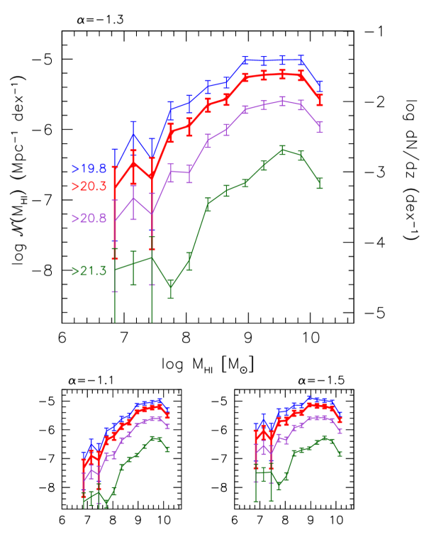
Figure 11: The expected distribution of the H i masses of high column density H i absorbing systems. The lines plus errorbars show the product of cross sectional area and space density, which translates to the number of expected absorbers per Mpc per decade of H i mass. The right axis shows the corresponding number of absorbers per unit redshift $dN/dz$.The different lines correspond to different column density limits, as indicated by the labels. The thick line corresponds to the classical DLA limit of $\log\mbox{$N_{\rm HI}$}>20.3$. The smaller panels show the effect of changing the slope of the low-mass slope of the H i mass function that is used to calculate the normalisation.

7.3 Surface brightness and Hubble type

The probability distribution function of $\mu_{B}^{25}$, the mean $B$-band surface brightness within the 25th mag arcsec^-2, is given in Fig. 12. Similar to the finding of Ryan-Weber, Webster, & Staveley-Smith (2003), we find that the cross section is dominated by galaxies with $\mu_{B}^{25}$ in the range 23 to 24 mag arcsec^-2. For reference, for our sample we find the median value of $\mu_{B}^{25}$ for $L_{*}$ galaxies is 23.6 mag arcsec^-2. At the bright end the distribution drops rapidly, showing that galaxies with high surface brightnesses contain a small fraction of the cross section. Toward dimmer galaxies, the distribution drops off slower. We find that 53 per cent of the DLA cross section is in galaxies dimmer than $\mu_{B}^{25}=23.6$ mag arcsec^-2. However, for 8 per cent of the galaxies in our sample no measurement of $\mu_{B}^{25}$ is available. Assuming that these galaxies have no measurement because of their low surface brightness, we are biased against LSB galaxies. Including these in our lowest $\mu_{B}^{25}$ bins increases the fraction of cross section in galaxies dimmer than $23.6$ mag arcsec^-2 to 64 per cent.

The measurement of optical surface brightness that we have used tends to understate the contribution of LSB galaxies to the DLA cross section. The reason for this is that if the surface brightness is measured within a fixed isophote, the radius of this isophote shrinks if the surface brightness decreases. $\mu_{B}^{25}$ is therefore always measured over the central brightest part of a galaxy, which naturally decreases the dynamic range in surface brightness measurements. A better alternative would be $\mu_{B}^{\rm eff}$, the effective surface brightness (the average surface brightness within the half-light radius), but unfortunately this parameter is only available for 40 per cent of the galaxies in the WHISP sample. For illustrative purposes, we can assign values of $\mu_{B}^{\rm eff}$ to those galaxies that have no measurements, by using the surface brightness–luminosity relation observed for nearby galaxies, for example by Cross & Driver (2002). For galaxies without $\mu_{B}^{\rm eff}$ we simply take the measurement of the galaxy closest in absolute magnitude in our sample. Thus, we find that the probability distribution of $\mu_{B}^{\rm eff}$ is much flatter at the LSB end than that of $\mu_{B}^{25}$. Specifically, we find that 71 per cent of the cross section is in galaxies dimmer than $\mu_{B}^{\rm eff}=22.0$ mag arcsec^-2, which corresponds to the peak of the distribution for $L_{*}$ galaxies. If an LSB galaxy is defined as having a surface brightness fainter than 1.5 mag arcsec^-2 below this value, we find that 44 per cent of the cross section is in LSB galaxies, in accord with the findings of Minchin et al. (2004). The fractional contribution of LSB galaxies to the DLA cross section is larger than their contribution to the H i mass density because their typical H i mass densities are lower than those observed in high surface brightness galaxies (e.g., de Blok & McGaugh, 1997). This is supported by the galaxy formation models of Mo, Mao, & White (1998), which indicate that cross-section-selected samples are weighted towards galaxies with high angular momentum (i.e., LSB galaxies). In conclusion, our data is not ideal to make firm statements about the contribution of LSB galaxies to the DLA cross-section. However, using the information we have available we can state that galaxies with surface brightness dimmer than that of a typical $L_{*}$ galaxy make up at least half of the cross section.

Turning now to the Hubble types, we see in Fig. 13 that late-type galaxies are preponderant in the distribution of DLA cross section. Earlier types are not negligible and the probability of identifying an S0 galaxy with a DLA is approximately a third of finding an Sc galaxy.

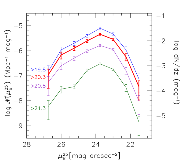
Figure 12: The expected distribution of the $B$-band surface brightness within the 25th mag isophote of host galaxies of high column density H i absorbing systems. The lines plus errorbars show the product of cross sectional area and space density, which translates to the number of expected absorbers per Mpc per magnitude. The right axis shows the corresponding number of absorbers per unit redshift $dN/dz$.The different lines correspond to different column density limits, as indicated by the labels. The thick line corresponds to the classical DLA limit of $\log\mbox{$N_{\rm HI}$}>20.3$.

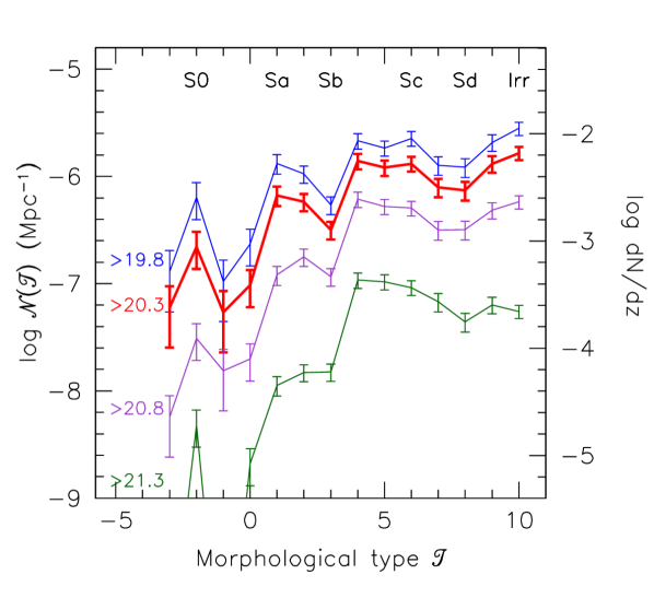
Figure 13: The expected distribution of the morphological types of host galaxies of high column density H i absorbing systems. The lines plus errorbars show the product of cross sectional area and space density, which translates to the number of expected absorbers per Mpc. The right axis shows the corresponding number of absorbers per unit redshift $dN/dz$.The different lines correspond to different column density limits, as indicated by the labels. The thick line corresponds to the classical DLA limit of $\log\mbox{$N_{\rm HI}$}>20.3$.

Table 3: Relative contribution to DLA cross section from different galaxies

Quantity	$<L_{*}/10$	$<L_{*}/5$	$<L_{*}$	$<2L_{*}$
$L$	0.45	0.58	0.87	0.96
$M_{\rm HI}$	0.22	0.37	0.81	0.96

Table 4: Expected properties of low-$z$ DLAs

Quantity	median	mean	logarithmic mean
$M_{B}$	$-18.1_{-1.9}^{+2.6}$	-19.2	-17.7
$\log\mbox{$M_{\rm HI}$}$ ($M_{\odot}$)	$9.3_{-0.7}^{+0.5}$	9.5	9.0
$b$ (kpc)	$7.6_{-5.0}^{+10.2}$	10.6	7.0

7.4 Impact parameters

Figure 14 shows the probability distribution of H i cross section in the $N_{\rm HI}$-$b$ plane, where $b$ is the impact parameter in kpc from the position of the observed column density to the centre of the galaxy. The WHISP sample was used to calculate the cross sectional area contributed by each element $d\mbox{$N_{\rm HI}$}db$ on a fine grid in the $N_{\rm HI}$-$b$ plane. We again used the type-specific H i mass functions to assign weights to each individual galaxy (see section 4). To increase the signal-to-noise in the figure, we smoothed the probability distribution with a Gaussian filter, which results in a final resolution of $\sigma=0.13$ dex in the $N_{\rm HI}$ direction and $\sigma=1.3$ kpc in the $b$ direction. The contour levels are chosen at 10, 30, 50, 70, and 90 per cent of the maximum value. The shaded area in the figure indicates the column density region that corresponds to DLA column densities.

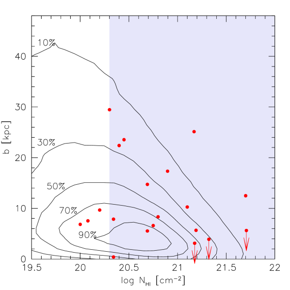
Figure 14: The two-dimensional probability distribution of H i cross section in the H i column density - impact parameter plane. The contours are calculated from our H i 21-cm maps and are drawn at 10, 30, 50, 70 and 90 per cent of maximum. The points are from DLA galaxy searches in the $z<1$ Universe. The shaded area shows the column density region corresponding to classical damped systems ($\log\mbox{$N_{\rm HI}$}>20.3$)

A few interesting features can be readily seen in Figure 14. The lowest contour illustrates that the highest H i column densities are very rarely seen at large galactocentric radii: there appears to be a strong correlation between $N_{\rm HI}$ and the maximum radius at which this is observed. The observational fact that the H i distribution in galaxies often shows a central depression can be seen by the compression of contours near $b=0$ kpc. Finally, this plot shows that the largest concentration of H i cross section in galaxies in the local Universe is in column densities in the range $20.3<\log\mbox{$N_{\rm HI}$}<20.8$ and impact parameters $b<7$ kpc.

The points in Figure 14 are the pairs of $N_{\rm HI}$ and $b$ measurements from the literature sample of low $z$ DLA galaxies from Table 2. If low $z$ DLAs are drawn from the same population of galaxies as those in our sample from the local Universe, we would expect the points to show the same distribution as the contours. Unfortunately, the statistics are too poor to calculate contours from the DLA galaxy data, but there seems to a qualitative agreement between the two data sets.

A more straightforward comparison between the DLA galaxies and local galaxy properties is presented in Figure 15, which shows the conditional probability distribution of impact parameter $b$ as a function of column density $N_{\rm HI}$. This figure is calculated by normalising at each value of $N_{\rm HI}$ in Figure 14 the distribution function of cross section as function of $b$ to the peak of the distribution. The solid line shows the median $b$ value as a function of $N_{\rm HI}$, the other lines show the 10th, 25th, 75th, 90th, and 99th percentiles, respectively. The literature values are again overplotted as points. Both in the $z=0$ data and in the DLA data, there is a weak correlation between $N_{\rm HI}$ and $b$. Rao et al. (2003) also noted the existence of this relation. The agreement between the points and the contours is remarkably good: 50 per cent of the literature values are within the 25th and 75th percentiles, and 75 per cent are within the 10th and 90th percentile contours. Based on our analysis, the expected median impact parameter of $\log\mbox{$N_{\rm HI}$}>20.3$ systems is 7.6 kpc, whereas the median impact parameter of identified $z<1$ DLA galaxies is 8.3 kpc. Although we are limited by small number statistics, a comparison between the contours and the points suggests that the observed number of very low $b$ systems is lower than expected. These identifications are the ones most likely to be missed due to the proximity of a the bright background QSO. Alternatively, if dust obscuration in DLA host galaxies is important, these low $b$ sight lines are expected to be the first to drop out of a flux limited quasar sample.

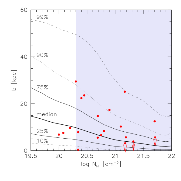
Figure 15: Conditional probability of impact parameter as a function of H i column density. The thick solid line shows the median impact parameter as calculated from our 21-cm emission line maps. The other lines show the 10th, 25th, 75th, 90th, and 99th percentiles, as indicated by the labels. The points are from DLA galaxy searches in the $z<1$ Universe.

A more detailed view of the distribution of impact parameters is presented in Figure 16, which shows the predicted probability distribution of $b$ for different column density cut-offs. The peak of the distribution for DLA column densities is at $b\sim 5$ kpc and the distribution drops rapidly toward higher values of $b$. The inset shows the probability distribution of $b$ above the DLA limit on a linear scale. For higher column densities, the probability distributions drop off even more rapidly, which again shows that it is extremely unlikely to encounter a high $N_{\rm HI}$ at a large separation from the centre of a galaxy. For DLA column densities, we find that 60 per cent of the host galaxies are expected at impact parameters $<10\,\rm kpc$ and 32 per cent at $<5\,\rm kpc$. Assuming no evolution in the properties of galaxy’s gas disk, these numbers imply that 37 per cent of the impact parameters are expected to be less than $1^{\prime\prime}$ for systems at $z=0.5$ and 48 per cent less than $1^{\prime\prime}$ at $z=1$. These numbers illustrate that very high spatial resolution imaging programs are required to successfully identify a typical DLA galaxy at $z\sim 1$.

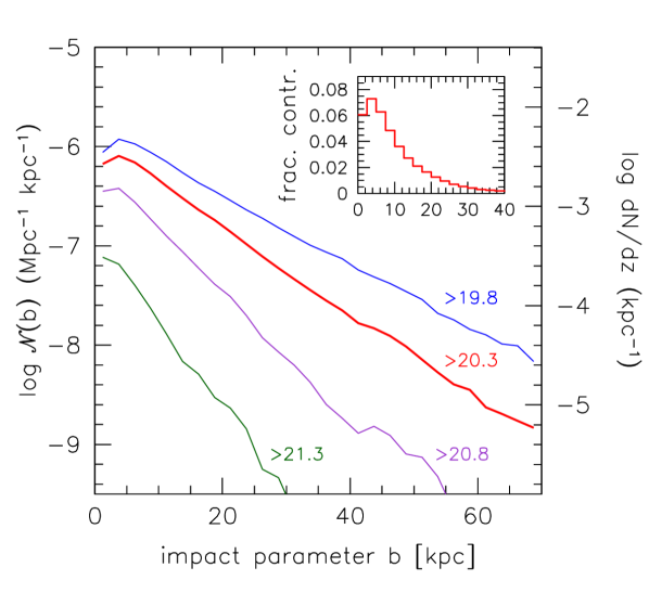
Figure 16: The probability distribution of impact parameter $b$ between the background QSO and the centre of a galaxy giving rise to H i absorption. The lines show the product of cross sectional area and space density, which translates to the number of expected absorbers per Mpc per kpc. The right axis shows the corresponding number of absorbers per unit redshift $dN/dz$.The different lines correspond to different column density limits, as indicated by the labels. The thick line corresponds to the classical DLA limit of $\log\mbox{$N_{\rm HI}$}>20.3$. The inset shows the probability distribution of $b$ for column densities $\log\mbox{$N_{\rm HI}$}>20.3$ on a linear vertical scale.

The intrinsic assumption in this comparison is that the low $z$ DLA galaxy sample is a fair cross-section selected sample. In reality the sample is a compilation of many surveys, using different selection techniques, and different resolutions and wave bands to image the galaxy. Keeping this limitation in mind, we conclude that the measured impact parameters and column densities of low $z$ DLA galaxies is in agreement with the hypothesis that DLA galaxies can be explained by the local galaxy population.

For completeness, we show in Figure 17 the expected probability distribution function of impact parameter $b$ at various column densities. Note the difference with the previous diagrams, where we plotted probability distribution functions above certain column density cut-offs. The right panel is the probability distribution function of column density at various values of $b$.

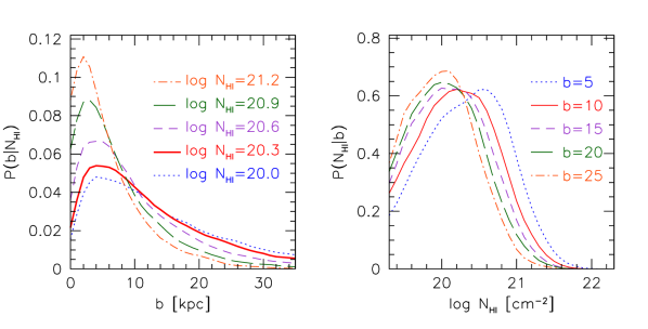
Figure 17: Left: Normalised probability distribution of impact parameter $b$ for different column densities. For H i column densities near the DLA limit of $2\times 10^{20}\,\rm cm^{-2}$, the most likely impact parameter to the host galaxy is $5\,h_{75}^{-1}$ kpc. Right: Normalised probability distribution of H i column density for different impact parameters $b$.

7.5 Linking DLA parameters to galaxy properties

We conclude our comparisons between DLA systems and local galaxies by looking at the combined probability distribution function of column density, impact parameter and host galaxy luminosity. In Fig. 18 we again show the $N_{\rm HI}$ and $b$ measurements from low-$z$ DLA galaxies from the literature, but this time the symbol size reflects the luminosity of the galaxies such that the symbol area scales in direct proportion to $L/L_{*}$. The contours represent the probabilities that the combined measurement of $N_{\rm HI}$ and $b$ is expected for a galaxy with luminosity $L>L_{*}$. For example, the thick solid line divides the diagram in two regions, above this line most host galaxies would be more luminous than $L_{*}$, below this line most would be less luminous than $L_{*}$. Apparently, the most luminous galaxies are most likely associated with high column density DLAs, at large impact parameters from the background QSOs.

The probability contours can be directly compared to the distribution of symbol sizes. Although the scatter is large, we see a general agreement between the points and the contours: below the 5 per cent line mostly low luminosity galaxies are found, and on the other hand, the two galaxies above the 70 per cent line are both galaxies with high luminosities. A similar diagram is presented in Fig. 19, but here contours indicate the probability that the host galaxy has an H i mass in excess of $M^{*}_{\rm HI}$. The conclusions from this figure are very similar as those from Figure 18.

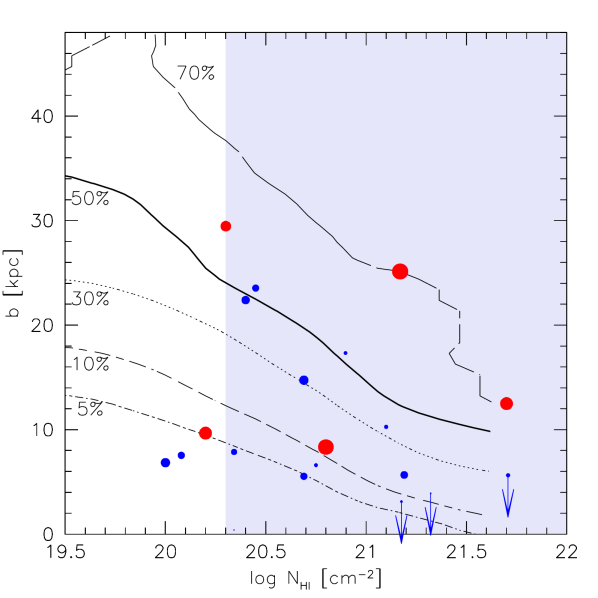
Figure 18: Probability distribution of optical luminosities of galaxies giving rise to H i absorption with column density $N_{\rm HI}$ and impact parameter $b$. The lines indicate the probability that the host galaxy is more luminous than an $L_{*}$ galaxy, and represent 5, 10, 30, 50 (thick line) and 70 per cent probabilities, from bottom to top. The points are from DLA galaxy searches and are the same as in Fig. 14 and Fig. 15, but here the symbol size represent intrinsic luminosity of the host galaxy. Red points indicate galaxies brighter than $L_{*}$, blue points are fainter than $L_{*}$.

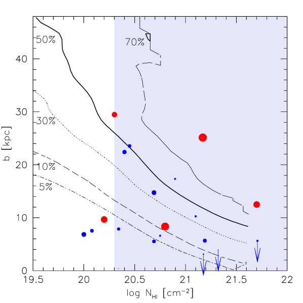
Figure 19: Probability distribution of H i masses of galaxies giving rise to H i absorption with column density $N_{\rm HI}$ and impact parameter $b$. The lines indicate the probability that the host galaxy has an H i mass in excess of $\mbox{$M_{\rm HI}$}^{*}$, and represent 5, 10, 30, 50 (thick line) and 70 per cent probabilities, from bottom to top. The points are the same as in Fig. 18

7.6 Comparison to models and simulations of DLAs

In order to compare our findings with numbers calculated in models of galaxy formation, we first transform the $B$-band luminosities of our WHISP galaxies into rotational velocities via the Tully-Fisher relation. We choose here to use the Tully-Fisher relation determined by Meyer et al. (2005), based on the HIPASS sample. Figure 20 shows the cumulative distribution of DLA redshift number density for galaxies with different rotational velocities $V_{\rm circ}$. We present the cumulative distribution because this representation is normally used in publications based on cosmological simulations, and can therefore be directly compared to those.

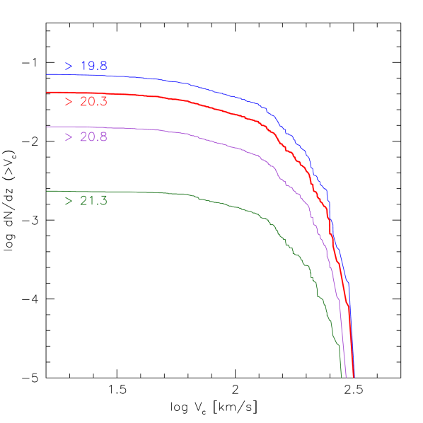
Figure 20: The cumulative redshift number density of DLAs in galaxies of different rotational velocities. The different lines correspond to different column density limits, the thick line is for $\log\mbox{$N_{\rm HI}$}>20.3$.

On the basis of semi-analytical models Okoshi & Nagashima (2005) find that the average virial velocity of a $z=0$ DLA is $V_{\rm vir}\sim 90\,\mbox{$\rm km\,s^{-1}$}$ and the average luminosity is $0.05L_{*}$. In their models, the fraction of DLA hosts in galaxies fainter than $L_{*}/10$ is 98 per cent, whereas we find that this fraction is only 41 per cent. Furthermore, they find that the typical impact parameter is 3 kpc, much smaller that our median value of 7.8 kpc. To make their results agree with observations of low-$z$ DLA galaxies, Okoshi & Nagashima (2005) propose that the masking effect where the DLA galaxies are contaminated by the point spread function of the QSO, hinders the identification of 60 per cent to 90 per cent of DLA galaxies with small impact parameters. The SPH simulations of Nagamine, Springel, & Hernquist (2004) also suggest that the relative contribution of low mass galaxies to the DLA cross section is very large: their cumulative contribution of redshift number density as a function of $V_{\rm circ}$ is steeper than what we find in Figure 20. These authors note that the $z=0$ results should be taken with caution because the mass resolutions that these results are based on are low and higher resolution SPH simulations are probably required to arrive at more precise results at $z=0$. Other work, such as that of Gardner et al. (2001), Mo, Mao, & White (1998, 1999), Haehnelt, Steinmetz, & Rauch (2000), and Maller et al. (2001) mostly concentrate on the high redshift ($z\sim 3$) DLA population and cannot be compared directly to our work, but also point to sub-$L_{*}$ galaxies as the major contributors to the DLA cross section. In conclusion, semi-analytical models and cosmological simulations generally over-predict the redshift number density contribution of low mass systems. A notable exception is the simple models of Boissier, Péroux, & Pettini (2003), which show that the peak and the median of the cross section distribution lies around $L_{*}$ galaxies. These models under-predict the importance of low mass systems, both in comparison with our results and in comparison with low $z$ DLA host galaxies.

From Figure 20 we find that the mean rotational velocity $V_{\rm circ}$ of a $z=0$ DLA is $111\,\mbox{$\rm km\,s^{-1}$}$ (the log-weighted mean $V_{\rm circ}$ is $95\,\mbox{$\rm km\,s^{-1}$}$). Note that the rotational velocities we measure are the peak velocities of the galaxies’ rotation curves, whereas in simulations galaxies are normally characterised by their virial velocity $V_{\rm vir}$. The ratio between these two values depends on the concentration index of the dark halo, but a typical value is $V_{\rm circ}\approx 1.4V_{\rm vir}$ (see Bullock et al., 2001), which implies that the log-weighted mean virial velocity of a $z=0$ DLA is approximately $70\,\mbox{$\rm km\,s^{-1}$}$. Using the relation between $V_{\rm circ}$ and the virial mass $M_{\rm vir}$ given by Bullock et al. (2001), we find that the mean total mass of a $z=0$ DLA would be $\approx 1.5\times 10^{11}\mbox{${\rm M}_{\odot}$}$.

8 Metal abundances of low redshift DLAs

In the previous section we have presented evidence that DLAs arise in the gas disks of galaxies such as those in the $z=0$ population. Measuring metallicities in DLAs therefore should provide information on abundances of the interstellar matter in galaxies. Determining DLA metallicities as a function of redshift will probe the history of metal production in galaxies over cosmic time. However, the metallicities typically measured in DLAs are low (around 1/13 solar), which is often taken as an indication that DLAs do not trace the general galaxy population, for which a mass-weighted mean metallicity of near-solar is expected at low redshift (see e.g., Pettini et al., 1997). In this section we present a more detailed analysis of the expected metallicities of DLAs, under the assumption that they arise in the gas disks of normal present day galaxies. We have no direct measurements of metal abundances for the complete sample of WHISP galaxies. However, we can make use of metallicity studies in other galaxies to statistically assign metallicities to our sample. Although this approach might introduce some degree of uncertainty in the results, it will help in understanding the observed metal abundance measurements in DLA systems. It should be kept in mind that the abundances of local galaxies are measured from emission lines arising in the photo-ionised gas, while the measurements in DLAs are from absorption lines in the neutral gas. However, recent work by Schulte-Ladbeck et al. (2005) shows that at least in one well-studied nearby galaxy the emission and absorption measurements of the same $\alpha$-elements are consistent.

8.1 The expected metallicities of DLAs at $z=0$

We take two different approaches to assigning metallicities to our sample of galaxies. The first approach is to adopt the well-established metallicity-luminosity ($Z-L$) relation for local galaxies and apply that to our sample. We choose to adopt the relation given by Garnett (2002) for oxygen abundances:

$$\log{\rm(O/H)}=-0.16M_{B}-6.4.$$ (11)

The results do not change significantly if instead we use the more recent $Z-L$ relation derived from SDSS imaging and spectroscopy of 53,000 galaxies (Tremonti et al., 2004). To convert the log(O/H) values to solar values we adopt the solar abundance of $12+\log{\rm(O/H)}=8.66$ from Asplund et al. (2004). The effect of abundance gradients as a function of galactocentric distance is taken into account by using the result from Ferguson, Gallagher, & Wyse (1998), who found a mean gradient of [O/H] of $-0.09\rm\,dex\,kpc^{-1}$ along the major axes of spiral galaxies. We assume that this gradient is equal for all galaxies and that it does not vary as a function of radius. We apply a simple geometrical correction to correct for inclined disks. Furthermore, we assume that Eq. 11 applies to the mean abundance measurement within $R_{25}$, which agrees with Garnett (2002). For each galaxy in our sample we scale the offset of the gradient such that the mean abundance measurement within $R_{25}$ fits the metallicity-luminosity relation. This approach intrinsically assumes that the [O/H] abundance gradients are independent of galaxy luminosity. To test the effect of this assumption on the calculation of expected metallicities of DLAs, we also take a second approach in which we adopt an [O/H] gradient that has both the intercept and slope varying with galaxy absolute magnitude. We fit straight lines to the relations found by Vila-Costas & Edmunds (1992) (their Figure 11) to find the varying slope and intercept. The two approaches depend on completely independent observations of metal abundances in local galaxies.

Every pixel in our 21-cm maps is assigned [O/H] values, based on the two procedures. Applying a similar method to that set out in section 7, we can now calculate the expected [O/H] distribution for cross-section selected samples, for different column density limits. The results are shown in Figure 21, where the solid lines refer to the first approach of fixed gradients, and the dashed lines refer to the varying gradients.

Figure 21: The probability distribution of oxygen abundance [O/H] of H i absorbers. The lines show the product of cross sectional area and space density, which translates to the number of expected absorbers per Mpc per decade. The right axis shows the corresponding number of absorbers per unit redshift $dN/dz$. The solid lines refer to the approach of assuming fixed [O/H] gradients and the the dashed lines refer to varying gradients (see text). The four different lines for each approach correspond to different column density limits, as indicated by the labels. The thick lines corresponds to the classical DLA limit of $\log\mbox{$N_{\rm HI}$}>20.3$.

Although the distributions peak at slightly different locations, it is obvious that the global trends are not strongly dependent on our assumptions on abundance gradients in disks. The main conclusion is that the metallicity distribution for H i column densities $\log\mbox{$N_{\rm HI}$}>20.3$ peaks around [O/H]=$-1$ to $-0.7$, much lower than the mean value of an $L_{*}$ galaxy of [O/H]$\approx 0$. Furthermore, we see a strong correlation between the peak of the [O/H] probability distribution and the H i column density limit: for H i column densities in excess of $\log\mbox{$N_{\rm HI}$}=21.3$, the expected peak of the distribution is at [O/H]=$-0.2$. This correlation is expected, since our assumed radial abundance gradients impose a relation between $N_{\rm HI}$ and [O/H]. Taking into account uncertainties in the H i mass function, in the $L-Z$ relation and in the abundance gradients in galaxies, we adopt a value of [O/H]$=-0.85\pm 0.2$ as a representative value for the median cross-section–weighted abundance of H i gas in the local Universe above the DLA column density limit.

8.2 Comparison to low-$z$ DLA metallicity measurements

It is interesting to compare this expected abundance of DLAs at $z=0$ to higher redshift values to see whether the measurements can be brought into agreement. The first evidence of evolution in DLA metallicities over cosmic time was presented by Kulkarni & Fall (2002), contrary to previous claims of no evolution (e.g., Pettini et al., 1997, 1999). This results was further established by an analysis of 125 DLA metallicity measurements over the redshift range $0.5<z<5$ by Prochaska et al. (2003), who reported significant evolution of $-0.26\pm 0.07\,\rm dex$ per unit redshift in the mean metallicity [M/H]. Kulkarni et al. (2005) compiled new metallicity measurements in four DLAs at $z<0.52$ and combined with literature measurements this study also finds evolution in [M/H] of $-0.18\pm 0.07\,\rm dex$ per unit redshift. The Prochaska et al. (2003) metallicity measurements are mostly based on $\alpha$-element abundances, whereas the Kulkarni et al. (2005) data is mostly based on Zn abundances. We refer to Kulkarni et al. (2005) for a discussion on why Zn is an appropriate choice as a metallicity indicator.

Before we compare our $z=0$ results to those for DLAs at higher redshifts, we discuss the different measurements of ‘mean metallicity’ that we can use to make the comparison. The first is to calculate the global interstellar metallicity $\bar{Z}$, defined as

$$\bar{Z}=\frac{\int\mbox{$N_{\rm HI}$}\mbox{$f(N_{\rm HI})$}Z(\mbox{$N_{\rm HI}$})d\mbox{$N_{\rm HI}$}}{\int\mbox{$N_{\rm HI}$}\mbox{$f(N_{\rm HI})$}d\mbox{$N_{\rm HI}$}}.$$ (12)

The reason that this equation gives a true measurement of the interstellar metallicity is that absorption lines are cross-section–selected, which implies that a correct weighting of different regions in absorbing systems is automatically taken into account, as is stressed by Kulkarni & Fall (2002). In practice, in DLA studies $\bar{Z}$ is normally calculated by taking the average over the metallicities of individual absorption-line systems weighted by their H i column densities. For our low $z$ data we can determine $\bar{Z}$ by simply taking the mass-weighted average of all mean metallicities of the WHISP galaxies:

$$\bar{Z}=\frac{\int\Theta(\mbox{$M_{\rm HI}$})\mbox{$M_{\rm HI}$}Z(\mbox{$M_{\rm HI}$})d\mbox{$M_{\rm HI}$}}{\int\Theta(\mbox{$M_{\rm HI}$})\mbox{$M_{\rm HI}$}d\mbox{$M_{\rm HI}$}},$$ (13)

where $\Theta(\mbox{$M_{\rm HI}$})$ is the H i mass function and $Z(\mbox{$M_{\rm HI}$})$ is the mean metallicity of a galaxy with H i mass $M_{\rm HI}$. We can calculate $Z(\mbox{$M_{\rm HI}$})$ by taking the column density-weighted metallicity of each WHISP galaxy, but only counting column densities above the DLA limit. Applying this method we find values of $\bar{Z}=0.58Z_{\odot}$ and $\bar{Z}=0.35Z_{\odot}$ for the fixed gradient and the variable gradient method, respectively. Kulkarni & Fall (2002) and Fukugita & Peebles (2004) applied similar techniques, but integrated over the optical luminosity function and found values of $\bar{Z}\approx 0.8Z_{\odot}$ and $\bar{Z}=0.83\pm 0.25Z_{\odot}$. The reason for these values being higher than ours is that these studies use one global metallicity measurement for each galaxy (which involves some radial averaging over the inner parts of galaxies), while our analysis takes into account radial abundance gradients over the whole H i gas disk. For the mean mass-weighted metallicity of H i gas with $\log\mbox{$N_{\rm HI}$}>20.3$ at $z=0$ we adopt the value of $\log\bar{Z}/Z_{\odot}=-0.35\pm 0.2$, where the errors again represent all uncertainties in arriving at this result.

The second measurement of metallicity is the cross-section–weighted average, which we will refer to as $\hat{Z}$. For DLAs, this measurement is simply the unweighted mean of the metallicities and represents a ‘typical’ metallicity of DLAs. For our $z=0$ sample, we can make use of the calculations presented in Fig. 21, which shows the cross-section–weighted [O/H] distribution of high column density H i gas in the local Universe. We find values of $\hat{Z}=0.36Z_{\odot}$ and $\hat{Z}=0.21Z_{\odot}$ for the fixed gradient and the variable gradient method, respectively, and hence adopt a value of $\log\hat{Z}/Z_{\odot}=-0.55\pm 0.2$, for the ‘typical’ metallicity of $z=0$ DLAs.

The third method stems directly from the way we presented the probability distribution of metallicity in Figure 21. As discussed above, we derive from this the cross-section–weighted median metallicity, for which we adopted $\log\tilde{Z}/Z_{\odot}=-0.85\pm 0.2$.

In Figure 22 we show the metallicities in DLAs as a function of redshift, extracted from the combined compilations by Prochaska et al. (2003) and Kulkarni et al. (2005). In amalgamating the two data sets we gave preference to Zn measurements for systems that occurred in both lists. The Kulkarni et al. (2005) data include many Zn measurements at low $z$, but a large fraction of those are upper limits. In order to take these limits into account appropriately, we applied the Kaplan-Meier estimator for randomly censored data sets, as implemented in the survival analysis package ASURV (Feigelson & Nelson, 1985). In six different redshift bins (approximately the same as those defined by Kulkarni et al. 2005) we calculate the mean $N_{\rm HI}$-weighted ($\bar{Z}$), the mean cross-section–weighted ($\hat{Z}$) and the median metallicities, as indicated by solid circles, triangles and stars, respectively. The errorbars are 1$\sigma$ statistical uncertainties as given by the Kaplan-Meier estimator. The long-dashed, short-dashed and dotted lines show the linear least squares fits to each set of measurements. The larger symbols at $z=0$ show our estimates of metallicities in the local Universe.

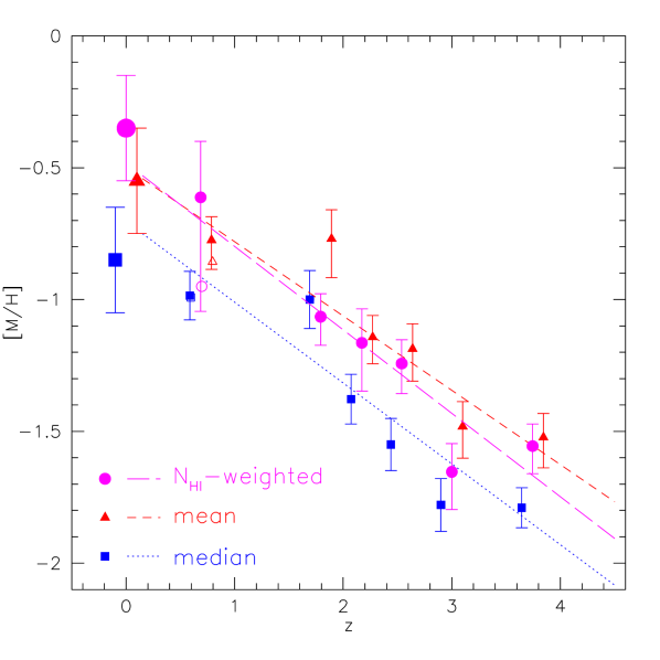
Figure 22: The metallicity [M/H] measurements in DLAs as a function of redshift. Data at redshifts $z>0$ are taken from Prochaska et al. (2003) and Kulkarni et al. (2005). Survival analysis has been used to calculate mean and median values because the data include many upper limits. The symbols refer to column density-weighted mean (filled circles), the cross-section–weighted mean (filled triangles), and median values (filled squares) in six redshift bins. The errorbars indicate 1 $\sigma$ statistical uncertainties. The lines are least squares fits to the $z>0$ data points. The points at $z=0$ are from our analysis as described in the text. The open symbols at $z\sim 0.6$ show the effect of excluding the X-ray metallicity measurement in Q0235+164. The squares and triangles are offset horizontally by $-0.1$ dex and $0.1$ dex, respectively.

For all measurements of metallicity a slope between $-0.25$ and $-0.3$ dex per unit redshift can be seen, in agreement with the findings of Prochaska et al. (2003) and Kulkarni et al. (2005), on whose compilations of data this figure is based. This increase in metallicity is consistent between the highest redshift points at $z\sim 4$ and the lowest points at $z\sim 0.6$. If we assume that DLAs arise in the gas disks of galaxies, where continued star formation causes a release of metals into the ISM, it seems reasonable to assume that this evolution in metallicity persists down to $z=0$. Note also that most models of cosmic chemical evolution predict a nearly exponential increase in metallicity as a function of redshift (c.f., Kulkarni & Fall, 2002). Given this assumption, we find from Figure 22 that the expected metallicity of DLAs at $z=0$ is in excellent agreement with our estimates from the local galaxy population: the $z=0$ extrapolations of all three lines are within the uncertainties of our estimates.

Kulkarni et al. (2005) have argued that the $N_{\rm HI}$-weighted DLA metallicities do not rise up to near-solar values at $z=0$. These authors find a DLA metal abundance of $-0.79\pm 0.18Z_{\odot}$ at $z=0$ using survival analysis, a factor of two lower than the Prochaska et al. (2003) extrapolation. This discrepancy lies mostly in the exclusion of the x-ray absorption based metallicity of the low-$z$ system AO 0235+164 (Junkkarinen et al., 2004). This system causes the large errorbars on the $z\sim 0.6$ points in Figure 22. The open symbols in Fig. 22 shows the effect of excluding AO 0235+164. The mean and median [M/H] are not affected much, but the $N_{\rm HI}$-weighted value drops by more than a factor of two because of the high $N_{\rm HI}$ measured in this system. Hence, if we only used the UV absorption measurements, we would find that our $N_{\rm HI}$-weighted $\bar{Z}$ in galaxies is a factor two higher than the extrapolated value from DLAs. Different authors disagree on whether it is fair to include this system (c.f., Chen, Kennicutt, & Rauch, 2005; Kulkarni et al., 2005), but at least it illustrates how poor the statistics are on low-$z$ abundance measurements. The lowest redshift bin includes 17 measurements (including AO 0235+164), of which five are limits. For illustration, if we calculate $\log\bar{Z}/Z_{\odot}$ at $z=0$ from 17 random sightlines through our galaxy sample, we find that the statistical error on this value is $-0.2+0.35$ dex, demonstrating that metallicity measurements based on small samples of DLAs are unavoidably marked by large uncertainties (see also Chen, Kennicutt, & Rauch, 2005).

Interestingly, we see that for local galaxies the $N_{\rm HI}$-weighted $\bar{Z}$ is higher than the mean $\hat{Z}$. Although the statistics are poor, it appears that for $z>1.5$ DLAs this is not the case. The origin of this difference might lie in the dust obscuration bias in DLAs: DLAs with the highest H i column densities and highest metallicities could be missed in magnitude-limited surveys as a consequence of their own extinction (see e.g. Fall & Pei, 1989, 1993; Ellison et al., 2001; Murphy & Liske, 2004; Vladilo & Péroux, 2005; Wild & Hewett, 2005, for a continued discussion on this issue). If, like at $z=0$, there is an intrinsic positive correlation between $N_{\rm HI}$ and metallicity, this bias would have a much higher effect on the $N_{\rm HI}$-weighted $\bar{Z}$ than on the mean $\hat{Z}$ of DLAs, causing the two measurements to be very similar in magnitude. In our local galaxy sample such a bias would not exist. The fact that we see a factor of two difference between the two values at $z=0$ and not for $z>1.5$ DLAs therefore is suggestive of dust obscuration introducing biases in DLA samples.

Finally, we comment on the scatter in the observed metallicity measurements in DLAs. From the probability distribution of [O/H] in Fig. 21 we find that the expected 1$\sigma$ scatter in cross section-selected metallicity measurements is 0.7 dex. A similar value is estimated by Chen, Kennicutt, & Rauch (2005). This is slightly larger than the typical scatter observed in metallicity measurements at high redshift of $\sim 0.5$ dex, illustrating that metallicity gradients in galaxy disks can easily explain the observed scatter in DLA metallicity measurements.

In conclusion, we find that the cross-section–weighted mean metallicity of local galaxies as well as the mass-weighted metallicity are in very good agreement with the hypothesis that DLAs arise in the H i disks of galaxies, provided that the metallicities in DLAs continue to evolve since $z=0.5$ with a rate similar to that observed between $z=0.5$ and $z=4$.

Before ending this section, we wish to comment briefly on the work of Chen, Kennicutt, & Rauch (2005), who presented similar conclusions based on Monte-Carlo simulations. These authors use average radial H i profiles for three types of galaxies and assume that the metallicity gradients in these galaxies are similar to what is found for their sample of DLAs. Their analysis does not take into account that galaxies over a large range in absolute magnitude contribute to the DLA cross section (see section 7.1), and effectively, only $L_{*}$ galaxies are considered. Therefore, the $L-Z$ relation is not taken into account in this analysis. Furthermore, in their analysis, the mean metallicity is measured over the whole gas disk out to the radius where 21-cm emission is normally detected, and not just over the region $\log\mbox{$N_{\rm HI}$}>20.3$. Since there is an intrinsic relation between $N_{\rm HI}$ and metallicity, this causes an underestimation of the mean $Z$ for DLAs. This explains why the Chen, Kennicutt, & Rauch (2005) estimate of the $N_{\rm HI}$-weighted mean $\bar{Z}=0.3Z_{\odot}$ is lower than our estimate.

9 Conclusions

In this paper we tested the hypothesis that DLA absorption lines observed in the spectra of background QSOs arise in gas disks of galaxies like those in the $z=0$ population. Since the H i column densities seen in DLA systems ($\mbox{$N_{\rm HI}$}>2\times 10^{20}$) are the same as those routinely observed in 21-cm emission line studies of local galaxies, we can make use of these observations to test the hypothesis. Thus, we used a sample of 355 high quality WSRT 21-cm emission line maps to calculate in detail the expected column density distribution function, the redshift number density, and the expected probability distribution functions of different galaxy parameters of the low redshift DLAs. We summarise the conclusions as follows:

1) The local galaxy population can explain the incidence rate of low redshift DLAs. There appears to be no evolution in the ‘cross section times space density’ or the mean free path between absorbers from $z\sim 1.5$ to $z=0$. Between the highest redshifts at which DLAs are found ($z\sim 4-5$) and the present time, the evolution in comoving incidence rate is only approximately a factor of two. We find that $dN/dz(z=0)=0.045\pm 0.006$.

2) Based on the local galaxy population it is expected that the DLA cross section is dominated by sub-$L_{*}$ galaxies ($87$ per cent). This agrees with the statistics of identified DLA host galaxies at low redshifts. 50 per cent of the low redshift DLAs should arise in galaxies with H i masses less than $\mbox{$M^{*}_{\rm HI}$}=6\times 10^{9}\,\mbox{${\rm M}_{\odot}$}$. The median $z=0$ DLA arises in a $L_{*}/7$ galaxy with an H i mass of $2\times 10^{9}\mbox{${\rm M}_{\odot}$}$.

3) The distribution of impact parameters and column densities agrees very well between local galaxies and low-$z$ DLA galaxies. The median impact parameter between the line of sight to a QSO and the centre of the galaxy giving rise to a DLA is 7.8 kpc. For systems at $z=0.5$ ($z=1$) we expect that $37$ per cent ($48$ per cent) have impact parameters less than $1^{\prime\prime}$. These findings support indications that optical surveys for DLA host galaxies miss identifications at very small impact parameters, because of the brightness of the QSO or because of blending due to too low spatial resolution. If obscuration of background QSOs by dust in DLA galaxies is important, this might also have the strongest effect at small impact parameters.

4) We combine our data set with the well-established luminosity-metallicity relation of galaxies and observed metallicity gradients in galaxy disks to estimate the expected metallicity distribution of low-$z$ DLAs. We find that the expected median metallicity of $z=0$ DLAs is approximately $1/7$ solar, in good agreement with observations of metal lines in DLAs. The mean mass-weighted metallicity of the interstellar matter in local galaxies above the DLA limit is approximately half solar. This is consistent with extrapolations from higher redshift measurements, although the $z=0$ extrapolated value has large uncertainties given the poor statistics from DLAs with redshifts approximately $z\approx 1.5$.

5) The column density distribution function $f(N_{\rm HI})$ in the local Universe can be fitted satisfactorily with a gamma distribution. A single power law is not a good fit. There is remarkably little evolution in the shape of $f(N_{\rm HI})$ from high $z$ to the present.

6) Most ($\approx 81$ per cent) of the cosmological mass density in H i at $z=0$ is locked up in column densities above the classical DLA limit of $\mbox{$N_{\rm HI}$}>2\times 10^{20}~{}\mbox{$\rm cm^{-2}$}$, the rest is mostly in column densities just below this limit. The fraction is consistent over the redshift range $z\sim 5$ to $z=0$.

References

- Asplund et al. (2004) Asplund M., Grevesse N., Sauval A. J., Allende Prieto C., Kiselman D., 2004, A&A, 417, 751
- Bouché et al. (2001) Bouché N., Lowenthal J. D., Charlton J. C., Bershady M. A., Churchill C. W., Steidel C. C., 2001, ApJ, 550, 585
- Boissier, Péroux, & Pettini (2003) Boissier, S., Péroux, C., & Pettini, M. 2003, MNRAS, 338, 131
- Bowen et al. (2001) Bowen, D. V., Huchtmeier, W., Brinks, E., Tripp, T. M., & Jenkins, E. B. 2001, A&A, 372, 820
- Bowen, Tripp, & Jenkins (2001) Bowen D. V., Tripp T. M., Jenkins E. B., 2001, AJ, 121, 1456
- Braun & Thilker (2004) Braun R., Thilker D. A., 2004, A&A, 417, 421
- Broeils (1992) Broeils, A. H. 1992, Ph.D. Thesis, University of Groningen
- Bullock et al. (2001) Bullock J. S., Kolatt T. S., Sigad Y., Somerville R. S., Kravtsov A. V., Klypin A. A., Primack J. R., Dekel A., 2001, MNRAS, 321, 559
- Burbidge et al. (1977) Burbidge G., Odell S. L., Roberts D. H., Smith H. E., 1977, ApJ, 218, 33
- Burbidge et al. (1996) Burbidge E. M., Beaver E. A., Cohen R. D., Junkkarinen V. T., Lyons R. W., 1996, AJ, 112, 2533
- Busswell et al. (2004) Busswell G. S., Shanks T., Frith W. J., Outram P. J., Metcalfe N., Fong R., 2004, MNRAS, 354, 991
- Carilli & Rawlings (2004) Carilli C. L., Rawlings S., 2004, NewAR, 48, 979
- Chen, Kennicutt, & Rauch (2005) Chen H.-W., Kennicutt R. C., Rauch M., 2005, ApJ, 620, 703
- Chen & Lanzetta (2003) Chen, H. & Lanzetta, K. M. 2003, ApJ, 597, 706
- Chengalur & Kanekar (2002) Chengalur, J. N. & Kanekar, N. 2002, A&A, 388, 383
- Churchill (2001) Churchill, C. W. 2001, ApJ, 560, 92
- Colbert & Malkan (2002) Colbert J. W., Malkan M. A., 2002, ApJ, 566, 51
- Cole et al. (2001) Cole S., et al., 2001, MNRAS, 326, 255
- Corbelli & Salpeter (1993) Corbelli E., Salpeter E. E., 1993, ApJ, 419, 104
- Corbelli & Bandiera (2002) Corbelli, E. & Bandiera, R. 2002, ApJ, 567, 712
- Cross & Driver (2002) Cross N., Driver S. P., 2002, MNRAS, 329, 579
- Curran et al. (2002) Curran S. J., Webb J. K., Murphy M. T., Bandiera R., Corbelli E., Flambaum V. V., 2002, PASA, 19, 455
- de Blok & McGaugh (1997) de Blok W. J. G., McGaugh S. S., 1997, MNRAS, 290, 533
- Dessauges-Zavadsky et al. (2003) Dessauges-Zavadsky, M., Péroux, C., Kim, T.-S., D’Odorico, S., & McMahon, R. G. 2003, MNRAS, 345, 447
- Dickey & Lockman (1990) Dickey J. M., Lockman F. J., 1990, ARA&A, 28, 215
- Ellison et al. (2001) Ellison, S. L., Yan, L., Hook, I. M., Pettini, M., Wall, J. V., & Shaver, P. 2001, A&A, 379, 393
- Fall & Pei (1989) Fall S. M., Pei Y. C., 1989, ApJ, 337, 7
- Fall & Pei (1993) Fall S. M., Pei Y. C., 1993, ApJ, 402, 479
- Feigelson & Nelson (1985) Feigelson E. D., Nelson P. I., 1985, ApJ, 293, 192
- Ferguson, Gallagher, & Wyse (1998) Ferguson A. M. N., Gallagher J. S., Wyse R. F. G., 1998, AJ, 116, 673
- Frith et al. (2003) Frith W. J., Busswell G. S., Fong R., Metcalfe N., Shanks T., 2003, MNRAS, 345, 1049
- Fukugita & Peebles (2004) Fukugita M., Peebles P. J. E., 2004, ApJ, 616, 643
- Gardner et al. (2001) Gardner J. P., Katz N., Hernquist L., Weinberg D. H., 2001, ApJ, 559, 131
- Fynbo, Møller, & Warren (1999) Fynbo, J. U., Møller, P., & Warren, S. J. 1999, MNRAS, 305, 849
- Garnett (2002) Garnett D. R., 2002, ApJ, 581, 1019
- Haehnelt, Steinmetz, & Rauch (1998) Haehnelt, M. G., Steinmetz, M., & Rauch, M. 1998, ApJ, 495, 647
- Haehnelt, Steinmetz, & Rauch (2000) Haehnelt, M. G., Steinmetz, M., & Rauch, M. 2000, ApJ, 534, 594
- Hopkins (2004) Hopkins A. M., 2004, ApJ, 615, 209
- Junkkarinen et al. (2004) Junkkarinen V. T., Cohen R. D., Beaver E. A., Burbidge E. M., Lyons R. W., Madejski G., 2004, ApJ, 614, 658
- Kanekar et al. (2001) Kanekar N., Chengalur J. N., Subrahmanyan R., Petitjean P., 2001, A&A, 367, 46
- Kauffmann (1996) Kauffmann G., 1996, MNRAS, 281, 475
- Khersonsky & Turnshek (1996) Khersonsky, V. K. & Turnshek, D. A. 1996, ApJ, 471, 657
- Kulkarni & Fall (2002) Kulkarni V. P., Fall S. M., 2002, ApJ, 580, 732
- Kulkarni et al. (2005) Kulkarni V. P., Fall S. M., Lauroesch J. T., York D. G., Welty D. E., Khare P., Truran J. W., 2005, ApJ, 618, 68
- Kulkarni et al. (2000) Kulkarni V. P., Hill J. M., Schneider G., Weymann R. J., Storrie-Lombardi L. J., Rieke M. J., Thompson R. I., Jannuzi B. T., 2000, ApJ, 536, 36
- Lacy et al. (2003) Lacy, M., Becker, R. H., Storrie-Lombardi, L. J., Gregg, M. D., Urrutia, T., & White, R. L. 2003, AJ, 126, 2230
- Lane, Briggs, & Smette (2000) Lane W. M., Briggs F. H., Smette A., 2000, ApJ, 532, 146
- Lane et al. (1998) Lane W., Smette A., Briggs F., Rao S., Turnshek D., Meylan G., 1998, AJ, 116, 26
- Lanzetta et al. (1991) Lanzetta K. M., McMahon R. G., Wolfe A. M., Turnshek D. A., Hazard C., Lu L., 1991, ApJS, 77, 1
- Le Brun et al. (1997) Le Brun, V., Bergeron, J., Boisse, P., & Deharveng, J. M. 1997, A&A, 321, 733
- Ledoux et al. (1998) Ledoux, C., Petitjean, P., Bergeron, J., Wampler, E. J., & Srianand, R. 1998, A&A, 337, 51
- Lin et al. (1996) Lin H., Kirshner R. P., Shectman S. A., Landy S. D., Oemler A., Tucker D. L., Schechter P. L., 1996, ApJ, 464, 60
- Liske et al. (2003) Liske J., Lemon D. J., Driver S. P., Cross N. J. G., Couch W. J., 2003, MNRAS, 344, 307
- Maller et al. (2001) Maller A. H., Prochaska J. X., Somerville R. S., Primack J. R., 2001, MNRAS, 326, 1475
- Maloney (1993) Maloney P., 1993, ApJ, 414, 41
- Meyer et al. (2004) Meyer M. J., et al., 2004, MNRAS, 350, 1195
- Meyer et al. (2005) Meyer M. J., et al., 2005, in prep.
- Milgrom (1988) Milgrom M., 1988, A&A, 202, L9
- Miller, Knezek, & Bregman (1999) Miller E. D., Knezek P. M., Bregman J. N., 1999, ApJ, 510, L95
- Minchin et al. (2004) Minchin R. F., et al., 2004, MNRAS, 355, 1303
- Mo, Mao, & White (1998) Mo H. J., Mao S., White S. D. M., 1998, MNRAS, 295, 319
- Mo, Mao, & White (1999) Mo H. J., Mao S., White S. D. M., 1999, MNRAS, 304, 175
- Møller et al. (2002) Møller, P., Warren, S. J., Fall, S. M., Fynbo, J. U., & Jakobsen, P. 2002, ApJ, 574, 51
- Murphy & Liske (2004) Murphy M. T., Liske J., 2004, MNRAS, 354, L31
- Nagamine, Springel, & Hernquist (2004) Nagamine K., Springel V., Hernquist L., 2004, MNRAS, 348, 421
- Nilson (1973) Nilson P., 1973, Uppsala general catalogue of galaxies
- Norberg et al. (2002) Norberg P., et al., 2002, MNRAS, 336, 907
- Noordermeer et al. (2004) Noordermeer E., van der Hulst J. M., Sancisi R., Swaters R., 2004, IAUS, 220, 287
- Noordermeer et al. (2005) Noordermeer E., van der Hulst J. M., Sancisi R., Swaters R., & van Albada T. S. 2005, A&A, 442, 137
- Okoshi & Nagashima (2005) Okoshi K., Nagashima M., 2005, ApJ, 623, 99
- Pei & Fall (1995) Pei, Y. C. & Fall, S. M. 1995, ApJ, 454, 69
- Péroux et al. (2001) Péroux, C., Storrie-Lombardi, L. J., McMahon, R. G., Irwin, M., & Hook, I. M. 2001, AJ, 121, 1799
- Péroux et al. (2002) Péroux, C., Irwin, M. J., McMahon, R. G., & Storrie-Lombardi, L. J. 2002, ASP Conf. Ser. 253: Chemical Enrichment of Intracluster and Intergalactic Medium, 501
- Péroux et al. (2003) Péroux, C., McMahon, R. G., Storrie-Lombardi, L. J., & Irwin, M. J. 2003, MNRAS, 346, 1103
- Péroux et al. (2004) Péroux C., Deharveng J., Le Brun V., Cristiani S., 2004, MNRAS, 352, 1291
- Péroux et al. (2005) Péroux, C., Dessauges-Zavadsky, M., D’Odorico, S., Kim, T., & McMahon, R. G. 2005, MNRAS, 363, 479
- Petitjean et al. (1996) Petitjean, P., Theodore, B., Smette, A., & Lespine, Y. 1996, A&A, 313, L25
- Pettini et al. (1997) Pettini M., Smith L. J., King D. L., Hunstead R. W., 1997, ApJ, 486, 665
- Pettini et al. (1999) Pettini M., Ellison S. L., Steidel C. C., Bowen D. V., 1999, ApJ, 510, 576
- Pettini et al. (2000) Pettini M., Ellison S. L., Steidel C. C., Shapley A. E., Bowen D. V., 2000, ApJ, 532, 65
- Prochaska & Wolfe (1997) Prochaska, J. X. & Wolfe, A. M. 1997, ApJ, 487, 73
- Prochaska & Wolfe (1998) Prochaska, J. X. & Wolfe, A. M. 1998, ApJ, 507, 113
- Prochaska et al. (2002) Prochaska, J. X., Gawiser, E., Wolfe, A. M., Quirrenbach, A., Lanzetta, K. M., Chen, H., Cooke, J., & Yahata, N. 2002, AJ, 123, 2206
- Prochaska et al. (2003) Prochaska J. X., Gawiser E., Wolfe A. M., Castro S., Djorgovski S. G., 2003, ApJ, 595, L9
- Prochaska & Herbert-Fort (2004) Prochaska, J. X. & Herbert-Fort, S. 2004, PASP, 116, 622
- Prochaska et al. (2005) Prochaska, J. X. , Herbert-Fort, S. & Wolfe, A. M. 2005, ApJ, in press
- Rao & Briggs (1993) Rao, S. & Briggs, F. 1993, ApJ, 419, 515
- Rao et al. (2003) Rao, S. M., Nestor, D. B., Turnshek, D. A., Lane, W. M., Monier, E. M., & Bergeron, J. 2003, ApJ, 595, 94
- Rao & Turnshek (2000) Rao, S. M. & Turnshek, D. A. 2000, ApJS, 130, 1
- Rao et al. (2005) Rao, S. M., Turnshek, D. A., & Nestor, D. B. 2005, ApJ, in press (astro-ph/0509469)
- Rosenberg & Schneider (2002) Rosenberg J. L., Schneider S. E., 2002, ApJ, 567, 247
- Rosenberg & Schneider (2003) Rosenberg, J. L. & Schneider, S. E. 2003, ApJ, 585, 256
- Ryan-Weber, Webster, & Staveley-Smith (2003) Ryan-Weber, E. V., Webster, R. L., & Staveley-Smith, L. 2003, MNRAS, 343, 1195
- Ryan-Weber, Webster, & Staveley-Smith (2005a) Ryan-Weber E. V., Webster R. L., Staveley-Smith L., 2005a, MNRAS, 356, 1600
- Ryan-Weber, Staveley-Smith, & Webster (2005b) Ryan-Weber E. V., Staveley-Smith L., & Webster, R. L. 2005b, MNRAS, in press
- Schaye (2001) Schaye, J. 2001, ApJL, 559, L1
- Schulte-Ladbeck et al. (2005) Schulte-Ladbeck R. E., König B., Miller C. J., Hopkins A. M., Drozdovsky I. O., Turnshek D. A., Hopp U., 2005, ApJ, 625, 79
- Steidel et al. (1997) Steidel, C. C., Dickinson, M., Meyer, D. M., Adelberger, K. L., & Sembach, K. R. 1997, ApJ, 480, 568
- Storrie-Lombardi, Irwin, & McMahon (1996) Storrie-Lombardi, L. J., Irwin, M. J., & McMahon, R. G. 1996, MNRAS, 282, 1330
- Storrie-Lombardi & Wolfe (2000) Storrie-Lombardi, L. J. & Wolfe, A. M. 2000, ApJ, 543, 552
- Swaters et al. (2002) Swaters R. A., van Albada T. S., van der Hulst J. M., Sancisi R., 2002, A&A, 390, 829
- Tammann (1985) Tammann, G. A. 1985, Star-Forming Dwarf Galaxies and Related Objects, 41
- Tremonti et al. (2004) Tremonti C. A., et al., 2004, ApJ, 613, 898
- Turnshek et al. (2001) Turnshek, D. A., Rao, S., Nestor, D., Lane, W., Monier, E., Bergeron, J., & Smette, A. 2001, ApJ, 553, 288
- Tytler (1987) Tytler D., 1987, ApJ, 321, 49
- van der Hulst, van Albada, & Sancisi (2001) van der Hulst J. M., van Albada T. S., Sancisi R., 2001, ASP Conf. Ser. 240: Gas and Galaxy Evolution, 240, 451
- Verheijen & Sancisi (2001) Verheijen, M. A. W. & Sancisi, R. 2001, A&A, 370, 765
- Vila-Costas & Edmunds (1992) Vila-Costas M. B., Edmunds M. G., 1992, MNRAS, 259, 121
- Vladilo & Péroux (2005) Vladilo, G., Péroux, C. 2005, A&A, in press
- Warren et al. (2001) Warren S. J., Møller P., Fall S. M., Jakobsen P., 2001, MNRAS, 326, 759
- Wild & Hewett (2005) Wild V., Hewett P. C., 2005, MNRAS, 361, L30
- Wolfe et al. (1986) Wolfe, A. M., Turnshek, D. A., Smith, H. E., & Cohen, R. D. 1986, ApJS, 61, 249
- Wolfe et al. (1995) Wolfe, A. M., Lanzetta, K. M., Foltz, C. B., & Chaffee, F. H. 1995, ApJ, 454, 698
- Wyithe, Agol, & Fluke (2002) Wyithe J. S. B., Agol E., Fluke C. J., 2002, MNRAS, 331, 1041
- Zwaan (2000) Zwaan M. A., 2000, PhD Thesis, University of Groningen
- Zwaan, Briggs, & Verheijen (2002) Zwaan, M., Briggs, F. H., & Verheijen, M. 2002, ASP Conf. Ser. 254: Extragalactic Gas at Low Redshift, 169
- Zwaan et al. (1997) Zwaan M. A., Briggs F. H., Sprayberry D., Sorar E., 1997, ApJ, 490, 173
- Zwaan et al. (2003) Zwaan, M. A., et al. 2003, AJ, 125, 2842
- Zwaan et al. (2005) Zwaan M. A., Meyer M. J., Staveley-Smith L., Webster R. L., 2005, MNRAS, 359, L30
- Zwaan, Verheijen, & Briggs (1999) Zwaan, M. A., Verheijen, M. A. W., & Briggs, F. H. 1999, Publications of the Astronomical Society of Australia, 16, 100