Probing the bispectrum at high redshifts using 21 cm HI observations

Abstract

Observations of fluctuations in the redshifted 21 cm radiation from neutral hydrogen (HI) are perceived to be an important future probe of the universe at high redshifts. Under the assumption that at redshifts $z\leq 6$ (Post-Reionization Era) the HI traces the underlying dark matter with a possible bias, we investigate the possibility of using observations of redshifted 21 cm radiation to detect the bispectrum arising from non-linear gravitational clustering and from non-linear bias. We find that the expected signal is $\sim 0.1{\rm mJy}$ at $325\,{\rm MHz}$ $(z=3.4)$ for the small baselines at the GMRT, the strength being a few times larger at higher frequencies ($610\,{\rm MHz},z=1.3$). Further, the magnitude of the signal from the bispectrum is predicted to be comparable to that from the power spectrum, allowing a detection of both in roughly the same integration time. The HI signal is found to be uncorrelated beyond frequency separations of $\sim 1.3{\rm MHz}$ whereas the continuum sources of continuum are expected to be correlated across much larger frequencies. This signature can in principle be used to distinguish the HI signal from the contamination. We also consider the possibility of using observations of the bispectrum to determine the linear and quadratic bias parameters of the HI at high redshifts, this having possible implications for theories of galaxy formation.

1 Introduction

Quantifying non-Gaussian features in the large-scale matter distribution is an important issue in cosmology. It is widely accepted that the large-scale structures originated from initially small density fluctuations which were a Gaussian random field. Non-Gaussian features arise as the fluctuations grow through the process of gravitational instability (eg. Peebles 1980), and quantifying these at various stages of the growth is expected to yield a significant amount of information. The three-point correlation function and its Fourier transform, the bispectrum, are the lowest order statistics sensitive to non-Gaussian features.

The determination of the three-point correlation function was pioneered by Peebles and Groth (1975) using the galaxies in the Lick and Zwicky angular catalogues. Later studies of the three point correlation function using galaxy surveys include Peebles (1981), Bean et al. (1983), Efstathiou & Jedrzejewski (1984), Hale-Sutton et. al. (1989), Jing, Mo & Borner (1991), Gaztanaga & Frieman (1994), Frieman & Gaztanaga (1994), Jing & Borner (1998). The recently completed Two -degree Field Galaxies Redshift Survey (2dfGRS) and the currently ongoing SDSS have been used to measure the galaxy three-point correlation function at an unprecedented level of accuracy (2dFGRS, Jing & Borner 2004; Kayo et al. 2004; Gaztanaga et al. 2005; SDSS ) allowing various issues like the luminosity and colour dependence to be addressed. There have recently been a few measurements of the bispectrum for the IRAS galaxies (Feldman et al. 2001; Scoccimarro et al. 2001) and for the 2dFGRS (Verde et al., 2002) which have (as discussed later) been used to estimate the galaxy bias.

All the measurements of the three-point correlation function or the bispectrum mentioned here are restricted to low redshifts $(z<1)$. This limitation arises because they are based on galaxy surveys which do not extend to very high redshifts. For example the 2dFGRS which is the largest completed redshift survey extends to a maximum redshift of around $z=0.3$. Further, a galaxy or quasar survey extending out to large redshifts ($z>1$) would select only the brightest objects which would be sparse in number. These objects would be distributed in the densest regions which are known to have a highly biased distribution and their distribution would not be representative of the underlying matter distribution. In this paper we discuss how observations of the redshifted $21$ cm emission from neutral hydrogen (HI) can be used to measure the bi-spectrum at high redshifts (ie. $z\sim 1$ and higher).

The HI density in the redshift range $1.7-5.5$ is known from observations of Ly-$\alpha$ absorption lines along lines of sight to quasars (1996; Storrie-Lombardi, & Wolfe 2000; Péroux et al. 2001; Prochaska, Herbert-Fort & Wolfe 2005). These observations indicate that $\Omega_{g}(z)$, the comoving density of neutral gas expressed as a fraction of the current critical density, has a value $\sim 10^{-3}$. Recent observations (Prochaska, Herbert-Fort & Wolfe, 2005) show that $\Omega_{g}(z)$ drops by about $25\%$ at $z=2.2-2.5$. Current observations of $\Omega_{g}(z)$ are consistent with no evolution at higher redshifts ($3\leq z\leq 5.5$). The bulk ($\sim 70\%$) of the HI resides in high column-density regions $(\geq 2.\times 10^{20}\,\rm cm^{-2})$ which are possibly the progenitors of present day galaxies. The redshifted 21 cm ($1420\,{\rm MHz}$) emission from this HI is present as a background radiation in radio observations at all frequencies below $1420\,{\rm MHz}$. The fluctuations in this background radiation arise from fluctuations in the HI density and from peculiar velocities at the redshift where the radiation originated (Bharadwaj, Nath and Sethi 2001, hereafter BNS). The possibility of detecting this holds the potential of being an important tool to probe the large-scale structures in the redshift range $z=1-6$. This is particularly significant in the context of the GMRT(Swarup et al., 1991) which operates in several bands in the frequency range of interest. It is also interesting to note that the fluctuations in the background HI radiation is expected to exceed the fluctuations in the CMBR by a factor of $10-100$ over the frequency range of interest (BNS).

Complex visibilities at different baselines and frequencies are the primary quantity measured in radio interferometric observations. Correlations between pairs of visibilities directly probe the three dimensional power spectrum of HI fluctuation at the redshift where the radiation originated. This has been studied in a series of papers (Bharadwaj and Sethi 2001; Bharadwaj and Pandey 2003, Bharadwaj & Srikant 2004) which develop the relation between visibility correlations and the HI power spectrum, and estimate the expected signal in the redshift range $z<6$ both analytically and using N-body simulations. This formalism has later been extended (Bharadwaj and Ali 2005) to quantify the expected HI visibility correlation signal over a large redshift range extending from the dark ages $(z\sim 100)$ to the present epoch. The possibility of using visibility correlations to probe the 3D HI power spectrum has also been considered by Morales and Hewitt (2004) while Zaldarriaga, Furlanetto and Hernquist (2004) propose the use of the angular power spectrum, both in the context of detecting the Epoch of Reionization (EOR) signal.

Bharadwaj and Pandey (2005) ( hereafter BP05) have, in a recent paper, investigated the possibility of using correlations between visibilities observed at three different baselines and frequencies to measure the bispectrum of HI fluctuations at the epoch of reionization. The HI distribution during the epoch of reionization will be determined more by the size, distribution and topology of the ionized regions and it is anticipated that this will not trace the underlying dark matter distribution. It is thus expected that the bispectrum of the HI during reionization will tell us more about the ionization process and less about the non-Gaussianity arising from the non-linear growth of density perturbation. In this paper we investigate how three visibility correlations can be used to study the HI bispectrum at redshifts $z<6$, where it is reasonable to assumed that the large scales HI distribution traces the dark matter with a possible bias.

We next briefly discuss what we can hope to learn from observations of non-Gaussianities in the HI. In perturbation theory the lowest order at which there is a non-zero three point correlation function is the second order (Fry 1984; Bharadwaj 1994). These predictions are expected to be valid on large scales which are weakly non-linear, and it is in principle possible to compare these with observations and test the currently accepted scenario for structure formation. The bispectrum has been perceived to be a more effective statistics for quantifying non-Gaussianity in the weakly non-linear regime and its theory has been developed in Fry (1994), Hivon et al. (1995), Matarrese et al. (1997), Verde et al. (1998), Scoccimarro et al. (1998), Scoccimarro, Couchman & Frieman (1999) and Scoccimarro et al. (2001). These investigations show that it possible to use observations of the bispectrum (or equivalently the three point correlation function) to determine the linear and quadratic bias parameters. This has been actually carried out using various galaxy surveys like the APM galaxies and the IRAS galaxies (Feldman et al. 2001; Scoccimarro et al. 2001). In a recent analysis Verde et al. (2002) have analysed the bispectrum of the 2dFGRS to conclude $b_{1}=1.04\pm 0.11$ for the linear bias parameter and $b_{2}=-0.054\pm 0.08$ for the quadratic bias parameter, indicating that the 2dFGRS galaxies are an unbiased tracer of the underlying dark matter. Further, the linear bias parameter was used in combination with the redshift distortion parameter $\beta\approx\Omega_{m0}^{0.6}/b_{1}$ measured from the same survey (Peacock et al., 2001) to determine the density of the universe $\Omega_{m0}=0.27\pm 0.06$. A new analysis of the three point correlation function of the 2dFGRS galaxies (Gaztanaga et al., 2005) confirms that the large-scale structures formed through gravitational instability starting from Gaussian initial conditions. The study concludes that the galaxies do not trace the underlying dark-matter distribution with $b_{1}=0.93^{0+.10}_{-0.08}$ and $c_{2}=b_{2}/B_{1}=-0.34^{+0.11}_{-0.08}$. Observations of the HI bispectrum would allow us to carry out such studies at redshifts $z>1$, providing further tests of the gravitational instability picture. Further, it would be possible to determine the bias of the HI at high redshifts, this being a potential probe of galaxy formation.

The cosmological evolution of the neutral hydrogen during the Epoch of Reionization $(z=6-20)$ and the pre-Reionization era $(z>20)$, and the expected redshifted 21 cm signal are topics of very intense research (eg. Scott and Rees 1990; Madau, Meiksin and Rees 1997; Gnedin & Ostriker 1997; Shaver et al. 1999; Tozzi et al. 2000; Iliev et al. 2003; Furlanetto,Sokasian. & Hernquist 2004; Miralda-Escude 2003; Zaldarriaga, Furlanetto and Hernquist 2004; Loeb & Zaldarriaga 2004; Bharadwaj & Ali 2004; Zaroubi & Silk 2004; Bharadwaj and Ali 2005; Bharadwaj and Pandey 2005; Barkana & Loeb 2005a; Barkana & Loeb 2005b; Barkana & Loeb 2005c; Bowman ,Morales & Hewitt 2005). We note that most of these papers have no direct bearing on the current work which is restricted to the Post-Reionization Era $(z<6)$ where it is reasonable to assume that the HI traces the dark matter, and the process of gravitational instability has progressed sufficiently to produce measurable departures from the Gaussian initial conditions. Subramanian & Padmanabhan (1993), Kumar, Padmanabhan & Subramanian (1995) and Bagla, Nath & Padmanabhan (1997) have considered the possibility of detecting HI at $z<6$ focusing on the possibility of detecting individual features corresponding to big HI clumps. Bagla and White (2003) have used N-body simulations to estimate the two-point statistics of the low $z$ HI signal.

We next present the structure of the paper. Section 2 reviews the formulae needed to calculate the visibility correlation signal expected from HI at high $z$. In Section 3. we present the results and discuss their implications.

Finally we note that, unless stated otherwise, we use the values $(\Omega_{m_{0}},\Omega_{\lambda_{0}},\Omega_{b}{h^{2}},h$) = ($0.3,0.7,0.02,0.7)$ for the cosmological parameters. Further, we use $\Omega_{g}=1\times 10^{-3}$ as a fiducial value and present results only for this throughout the paper.

2 Calculating the HI visibility correlation signal

The quantity measured in radio-interferometric observations is the complex visibility $V({\bf U},\nu)$ which records only the angular fluctuations of the specific intensity $I_{\nu}$ on the sky. This is measured for every pair of antennas in a radio-interferometric array. For any pair of antennas at a separation ${\bf d}$, we refer to the two dimensional vector ${\bf U}={\bf d}/\lambda$ as a baseline. In this paper it has been assumed that all the antennas in the array are coplanar, and that the antennas all point vertically up wards in the direction ${\bf m}$ with ${\bf m\cdot{\bf U}}=0$. Further, the individual antennas are assumed to have a Gaussian beam pattern $A(\theta)=e^{-\theta^{2}/\theta_{0}^{2}}$ with $\theta_{0}\ll 1$ (in radians) i.e. the beam width $\theta_{0}$ of the antennas is small, and the part of the sky which contributes to the signal can be well approximated by a plane.

Fluctuations in the high redshift HI density contributes to the visibilities measured at all frequencies below $1420\,{\rm MHz}$. Following BP05 we consider the contribution from the HI signal to the correlations

$${\rm S}_{2}({\bf U}_{1},{\bf U}_{2},\Delta\nu)=\langle V({\bf U}_{1},\nu+\Delta\nu)V({\bf U}_{2},\nu)\rangle$$ (1)

and

$${\rm S}_{3}({\bf U}_{1},{\bf U}_{2},{\bf U}_{3},\Delta\nu_{1},\Delta\nu_{2}) = \langle V({\bf U}_{1},\nu+\Delta\nu_{1})V({\bf U}_{2},$$ (2)

$$\nu+\Delta\nu_{2})V({\bf U}_{3},\nu)\rangle$$

expected between the visibilities at different baselines and frequencies. Here the two visibility correlation function ${\rm S}_{2}({\bf U}_{1},{\bf U}_{2},\Delta\nu)$ denotes the correlation expected between the visibilities measured at two different baselines ${\bf U}_{1}$ and ${\bf U}_{2}$ one at the frequency $\nu$ and the other at $\nu+\Delta\nu$. It should be noted that although we have shown ${\rm S}_{2}$ as an explicit functions of the frequency differences $\Delta\nu$ only, it also depends on the central value $\nu$ which is not shown as an explicit argument. The value of $\nu$ will be clear from the context of the discussion. Further, throughout our analysis we assume that all frequency differences are much smaller than the central frequency ie. $\Delta\nu/\nu\ll 1$. The definition of the three visibility correlation ${\rm S}_{3}$ closely follows that of ${\rm S}_{2}$.

It has been shown that the two-visibility correlation probes the power spectrum of HI fluctuations (Bharadwaj and Sethi 2001, Bharadwaj and Ali 2005) and the three visibility correlation the bispectrum (Bharadwaj and Pandey 2005). Considering ${\rm S}_{2}({\bf U}_{1},{\bf U}_{2},\Delta\nu)$ first, we note that it has a significant value only when $\mid{\bf U}_{2}+{\bf U}_{1}\mid<(\pi\theta_{0})^{-1}$. Therefore we restrict the analysis to ${\bf U}_{1}=-{\bf U}_{2}={\bf U}$ which we denote as ${\rm S}_{2}({\bf U},\Delta\nu)$. This is related to the redshift space HI power spectrum $P_{\rm HI}({\bf k})$ as

$${\rm S}_{2}(U,\Delta\nu)=\frac{\bar{I}^{2}_{\nu}\theta_{0}^{2}}{2r_{\nu}^{2}}\int_{0}^{\infty}dk_{\parallel}\,P_{{\rm HI}}({\bf k})\cos(k_{\parallel}r_{\nu}^{{}^{\prime}}\Delta\nu)\,.$$ (3)

where $r_{\nu}$ is the comoving distance to the HI whose $1420{\rm\,MHz}$ radiation is observed at a frequency $\nu$, $r_{\nu}^{{}^{\prime}}=dr_{\nu}/d\nu$, ${\bf k}=k_{\parallel}{\bf m}+(2\pi/r_{\nu}){\bf U}$ and $\bar{I}_{\nu}=2.5\times 10^{2}\,\frac{\rm Jy}{\rm sr}\,\left(\frac{\Omega_{b}h^{2}}{0.02}\right)\left(\frac{0.7}{h}\right)\frac{H_{0}}{H(z)}$. A point to note is that $P_{\rm HI}({\bf k})$ includes the effects of redshift space distortions, and is therefore anisotropic along the the line of sight ${\bf m}$. We further note that ${\rm S}_{2}$ is real and isotropic ie it does not depend on the direction of the baseline ${\bf U}$ whereby we can write ${\rm S}_{2}(U,\Delta\nu)$.

Considering the three visibility correlation ${\rm S}_{3}({\bf U}_{1},{\bf U}_{2},{\bf U}_{3},\Delta\nu_{1},\Delta\nu_{2})$ next, this has a significant value only if $\mid{\bf U}_{1}+{\bf U}_{2}+{\bf U}_{3}\mid\leq(\pi\theta_{0})^{-1}$. We therefore restrict our analysis to only those combinations of baselines for which ${\bf U}_{1}+{\bf U}_{2}+{\bf U}_{3}=0$. Further ${\rm S}_{3}$ is real and it depends only on the shape and size of the triangle which is completely specified by the magnitude of the three baselines $(U_{1},U_{2},U_{3})$. We have

$${\rm S}_{3}(U_{1},U_{2},U_{3},\Delta\nu_{1},\Delta\nu_{2}) = \frac{\bar{I}^{3}_{\nu}\,\theta_{0}^{2}}{12\,\pi\,r_{\nu}^{4}}\int d{k_{1\parallel}}d{k_{2\parallel}}\cos[({k_{1\parallel}}\,\Delta\nu_{1}$$ (4)

$$+ {k_{2\parallel}}\Delta\nu_{2})r_{\nu}^{{}^{\prime}}]\,\times B_{{\rm HI}}({\bf k}_{1},{\bf k}_{2},{\bf k}_{3})$$

where ${\bf k}_{1}={k_{1\parallel}}{\bf m}+(2\pi/r_{\nu}){\bf U}_{1}$, ${\bf k}_{2}={k_{2\parallel}}{\bf m}+(2\pi/r_{\nu}){\bf U}_{2}$, ${\bf k}_{3}=-({k_{1\parallel}}+{k_{2\parallel}}){\bf m}+(2\pi/r_{\nu}){\bf U}_{3}$ and $B_{\rm HI}({\bf k}_{1},{\bf k}_{2},{\bf k}_{3})$ is the redshift space HI bispectrum.

It is next necessary to specify the form of the redshift space HI power spectrum $P_{{\rm HI}}$ and bispectrum $B_{{\rm HI}}$. Fluctuations in the redshifted HI radiation arise from fluctuations in the HI density and from HI peculiar velocities, and it is necessary to include both these effects in $P_{{\rm HI}}$ and $B_{{\rm HI}}$. We assume that the HI traces the dark matter with a possible bias, and retain terms upto the quadratic order in the relation between the fluctuations in the HI density $\delta_{\rm HI}$ and the fluctuations in the dark matter density $\delta$

$$\delta_{\rm HI}=b_{1}\delta+\frac{b_{2}}{2}\delta^{2}$$ (5)

where $b_{1}$ and $b_{2}$ are the linear and quadratic bias parameters respectively. A non-zero $b_{2}$ would indicate nonlinear biasing of HI distribution with respect to underlying mass distribution. It is also assumed that the peculiar velocities are determined by the dark matter which dominates the dynamics.

The HI power spectrum $P_{\rm HI}({\bf k})$ is related to the real space dark matter power spectrum $P(k)$ as

$$P_{\rm HI}({\bf k})=b_{1}^{2}\bar{x}_{{\rm HI}}^{2}(1+\beta\mu^{2})^{2}P(k)\,$$ (6)

$\mu$ being the cosine of the angle between ${\bf k}$ and the line of sight ${\bf m}$, and $\beta=f(\Omega_{m})/b_{1}\approx\Omega_{m}^{0.6}/b_{1}$ is the linear distortion parameter. The term $(1+\beta\mu^{2})^{2}$ in equation (6) incorporates the effect of the peculiar velocities, and $\bar{x}_{{\rm HI}}$ is the mean hydrogen neutral fraction. Converting $\Omega_{gas}$ to the mean neutral fraction $\bar{x}_{{\rm HI}}=\bar{\rho}_{{\rm HI}}/\bar{\rho}{{\rm H}}=\Omega_{gas}/\Omega_{b}$ gives us $\bar{x}_{{\rm HI}}=50\Omega_{gas}h^{2}(0.02/\Omega_{b}h^{2})$ or $\bar{x}_{{\rm HI}}=2.45\times 10^{-2}$. It should be noted that $\mid\delta\mid\ll 1$ and terms higher than $\delta^{2}$ have been dropped in the power spectrum.

For the HI bispectrum we assume

$$B_{{\rm HI}}({\bf k}_{1},{\bf k}_{2},{\bf k}_{3}\,,z)=\bar{x}^{3}_{{\rm HI}}\,B_{s}({\bf k}_{1},{\bf k}_{2},{\bf k}_{3}\,,z)$$ (7)

where $B_{s}$ is the redshift space bispectrum calculated by Verde et al. (1998). We have used the form of $B_{s}$ given in equation (11) of (Verde et al., 1998), the expression being quite lengthy we do not reproduce it here. We note that $B_{s}({\bf k}_{1},{\bf k}_{2},{\bf k}_{3})$ has a quadratic dependence on the dark matter power spectrum $P(k)$, it depends on the bias parameters $b_{1}$ and $b_{2}$, and on the parameters of the background cosmological model. The value of $B_{s}$ also depends on the shape of the triangle formed by $({\bf k}_{1},{\bf k}_{2},{\bf k}_{3})$.

The fact that the neutral hydrogen is in discrete clouds makes a contribution which we do not include here. This effect originates from the fact that the HI emission line from individual clouds has a finite width, and the visibility correlation is enhanced when $\Delta\nu$ is smaller than the line-width of the emission from the individual clouds. Another important effect not included here is that the fluctuations become significantly non-linear at low $z$. Both these effects have been studied for the power spectrum using simulations (Bharadwaj & Srikant, 2004).

The simple analytic treatment adopted here suffices for the purposes of this paper where the main focus is to estimate the magnitude and the nature of the HI signal, and to investigate the feasibility of using such observations to probe structure formation at high redshifts.

3 Results and Discussion

We present results for the two and three visibility correlation signal expected from HI at high $z$. In calculating the expected signal we have used the GMRT parameters, but it is straight forward to scale the results presented here to make the visibility correlation predictions for other radio telescopes. The only telescope parameter which enters equations (3) and (4) is $\ \theta_{0}\$, which is the beam size of the individual antenna in the array. Further, it should be noted that $\ \theta_{0}\approx 0.6\times\theta_{\rm FWHM}\$. The value of $\theta_{0}$ will depend on the physical dimensions of the antennas and the wavelength of observation. For the GMRT $\ \theta_{0}=1^{\circ}\$ at $\ 325\,{\rm MHz}$. We scale this using $\theta_{0}\propto\lambda$ to obtain $\ \theta_{0}\$ corresponding to different observation frequencies. We note that the smallest baseline at the GMRT is a little smaller than $U=100$ while the largest is around $U\sim 10,000$, and we present results for $U$ in the range $10-10,000$. It may be noted that unless mentioned otherwise ,we use the values ($b_{1}$ , $b_{2}$ )$=$ (1.0 , 0.5) for the bias parameters.

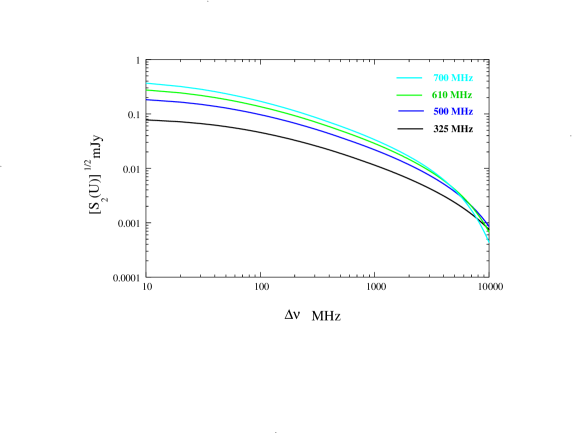
Figure 1: This shows the expected two visibility correlation signal $[{\rm S}_{2}(U,0)]^{1/2}$ as a function of $U$ for the different values of the central frequency shown in the figure.

Figure 1 shows the $[{\rm S}_{2}(U,0)]^{1/2}$, the two visibility correlation signal expected when the two visibilities are at the same baseline and frequency. The signal is strongest at small baselines, and it is around $0.1\,{\rm mJy}$ at $325\,{\rm MHz}$ ie. $(z=3.4)$. The signal falls with increasing $U$, and the $U$ dependence reflects the shape of the power spectrum. Further, the signal increases with increasing central frequency or decreasing redshift,. This is a consequence of the fact that the matter power spectrum grows with time.

To estimate the magnitude of the expected three visibility correlation signal ${\rm S}_{3}(U_{1},U_{2},U_{3},\Delta\nu_{1},\Delta\nu_{2})$, we first restrict our analysis to equilateral triangles for which the size of the baseline $U$ completely specifies the triangle, We further restrict our analysis to $\Delta\nu_{1}=\Delta\nu_{2}=\Delta\nu$ in which case we can use the notation ${\rm S}_{3}(U,\Delta\nu)$. The ratio $\ \frac{[{\rm S}_{3}(U,0)]^{1/3}}{[{\rm S}_{2}(U,0)]^{1/2}}\$ (Figure 2) quantifies the relative strength of ${\rm S}_{3}$ as a fraction of ${\rm S}_{2}$. The first point to note is that the three visibility correlation signal is comparable in magnitude to the two visibility correlation signal. The ratio of the signal strengths is of order unity for the small baselines ($U\leq 1000$) at $325\,{\rm MHz}$ and it is somewhat higher at higher frequencies. Further, ${\rm S}_{3}^{1/3}$ falls faster than ${\rm S}_{2}^{1/2}$ with increasing $U$. It is possible to understand both these features of ${\rm S}_{3}$ in terms of the fact that the bispectrum is quadratic in the power spectrum whereby it grows faster with time and it has a steeper $k$ dependence at large $k$.

The bispectrum $B_{s}({\bf k}_{1},{\bf k}_{2},{\bf k}_{3})$ depends on the shape and size of the triangle formed by ${\bf k}_{2},{\bf k}_{2}$ and ${\bf k}_{3}$. This dependence varies with the bias parameters $(B_{1},b_{2})$, and this can be used to observationally determine the values of the bias parameters. To study how the shape and bias dependence manifests itself in ${\rm S}_{3}$, we have considered bilateral triangles for which two sides are of length $U$ with opening angle $120^{\circ}$ and the third side of length $\sqrt{3}U$. We study the ratio $[{\rm S}_{3}(U,\Delta\nu)]^{1/3}_{\rm E}/[{\rm S}_{3}(U,\Delta\nu)]^{1/3}_{\rm B}$ for $\Delta\nu=0$ where the subscripts ${\rm E}$ and ${\rm B}$ refer to equilateral and bilateral triangles respectively. Figure 3 shows the results at $610{\rm MHz}$ $(z=1.3)$, the behaviour at other frequencies is similar. We find that ${\rm S}_{3}$ does not show any significant dependence on the triangle shape at baselines smaller than $U\sim 1000$. There is a shape dependence at larger baselines where ${\rm S}_{3}$ decreases faster for the equilateral triangles than for the bilateral triangles. Further, the ratio has a distinct dependence on the values of the bias parameters. The first point to note is that the ratio is independent of $b_{1}$ for $b_{2}=0$. For other values of $b_{2}$ we find that the $U$ dependence of the ratio $[{\rm S}_{3}(U,0)]^{1/3}_{\rm E}/[{\rm S}_{3}(U,0)]^{1/3}_{\rm B}$ at the large baselines is sensitive to both $b_{1}$ and $b_{2}$. It should, in principle, be possible to use observations of the shape dependence of ${\rm S}_{3}$ to determine the bias parameters.

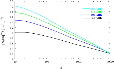
Figure 2: This shows the ratio $\frac{[{\rm S}_{3}(U,0)]^{1/3}}{[{\rm S}_{2}(U,0)]^{1/2}}$ as a function of $U$ for the different values of the central frequency shown in the figure.

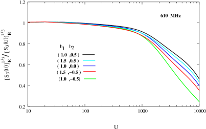
Figure 3: This shows the ratio $[{\rm S}_{3}(U,\Delta\nu)]^{1/3}_{E}/[{\rm S}_{3}(U,\Delta\nu)]^{1/3}_{B}$ for $\Delta\nu=0$, where $E$ refers to equilateral triangles and $B$ to bilateral triangles. Two sides of the bilateral triangle are $U$ (at $120^{\circ}$) and the third is $\sqrt{3}U$. The central frequency is $610{\rm MHz}$. The results are for the different combinations of the bias parameters $(b_{1},b_{2})$ shown in the figure.

We next consider the correlation between visibilities at different frequencies. The results are presented at fixed values of the baselines, and Figures 4 and 5 show  $[{\rm S}_{2}(U,\Delta\nu)]^{1/2}$ and $[{\rm S}_{3}(U,\Delta\nu)]^{1/3}$ respectively, both at the central frequency of $610\,{\rm MHz}$. We find that the correlations decay rapidly as the frequency separation $\Delta\nu$ is increased. We have ${\rm S}(U,\delta\nu)=0$ at $\Delta\nu\sim 1.3\,{\rm MHz}$ for $U=100$, and there is a weak anticorrelation ${\rm S}_{2}<0$ for larger $\Delta\nu$. The visibilities at larger baselines get decorrelated faster with increasing $U$, and the zero crossing is at $\sim 0.7\,{\rm MHz}$ at $U=100$. The three visibility correlation shows a similar behavior, the main difference being that $[{\rm S}_{3}(U,\Delta\nu)]^{1/3}$ decays much faster than $[{\rm S}_{2}(U,\Delta\nu)]^{1/2}$ with increasing $\Delta\nu$. It may be noted that the overall behavior is similar at other values of the central frequency, with the difference that ${\rm S}_{2}$ and ${\rm S}_{3}$ decay faster with increasing $\Delta\nu$ at lower values of the central frequency.

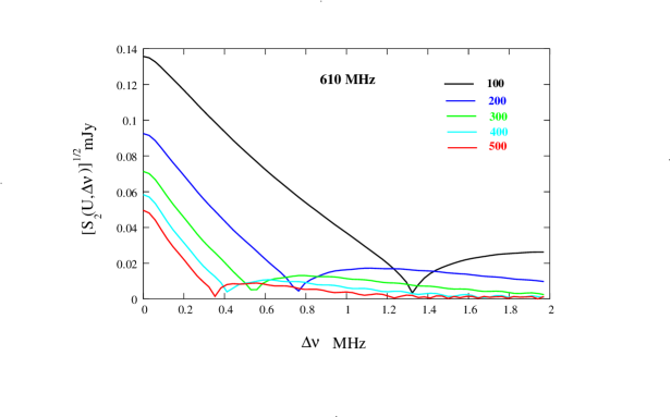
Figure 4: This shows the expected two visibility correlation signal $[{\rm S}_{2}(U,\Delta\nu)]^{1/2}$ as a function of $\Delta\nu$ for the different values of $U$ shown in the figure at a central frequency of $610{\rm\,MHz}$

.

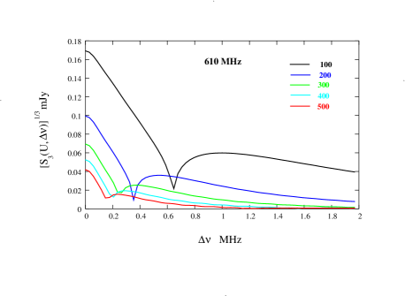
Figure 5: This shows the expected three visibility correlation signal $[{\rm S}_{3}(U,\Delta\nu)]^{1/3}$ as a function of $\Delta\nu$ for the different values of $U$ shown in the figure at a central frequency of $610{\rm\,MHz}$

.

An important issue which we have not addressed here in any detail is the extraction of the HI signal from various contaminants which are expected to dominate at low frequencies. The issue of extracting the redshifted 21 cm signal has received considerable attention (eg. Shaver et al. 1999; DiMatteo. et al. 2004 ; Oh et al. 2003;Morales and Hewitt 2004 ; Zaldarriaga, Furlanetto and Hernquist 2004 ; Cooray & Furlanetto 2004 ; Santos et al. 2005 ; Wang , Tegmark ,Santos & Knox 2005; Morales ,Bowman & Hewitt 2005). The contribution from the continuum sources of contamination at two different frequencies is expected to be correlated even at large $\Delta\nu$, whereas the HI signal is found to be uncorrelated beyond something like $1.3\,{\rm MHz}$ or even less depending on the value of $U$. It is then, in principle, straightforward to fit the visibility correlations ${\rm S}_{2}$ and ${\rm S}_{3}$ at large $\Delta\nu$ and remove any slowly varying component thereby separating the contaminants from the HI signal. We also use this opportunity to note that this is a major advantage of using visibility correlations as compared to the angular power spectrum which has been found to have substantial correlations even at two frequencies separated by $\sim 10\,{\rm MHz}$ (Santos et al., 2005).

System noise is inherent in all radio interferometric observations. System noise and the observation time needed to detect the HI signal is another important issue. Here we briefly discuss the signal to noise ratio and approximate integration time required to detect the HI signal for ${\rm S}_{2}$ and ${\rm S}_{3}$. We consider an array of $N$ antennas, the observations lasting a time duration $t$, with frequency channels of width $\delta\nu$ spanning a total bandwidth $B$. It should be noted that the effect of a finite channel width $\delta\nu$ has not been included in our calculation which assumes infinite frequency resolution. This effect can be easily included by convolving our results for the visibility correlation with the frequency response function of a single channel. Preferably, $\delta\nu$ should be much smaller than the frequency separation at which the visibility correlation become uncorrelated. We use $\cal S$ denote the frequency separation within which the visibilities are correlated, and beyond which they become uncorrelated.We use ${\rm N}_{2}$ and ${\rm N}_{3}$ to denote the rms. noise in ${\rm S}_{2}$ and ${\rm S}_{3}$. we have assumed that thermal noise are Gaussian random fields. It is well known that ${\rm N}_{2}=\left(\frac{2k_{B}T_{SYS}}{A_{ef}}\right)^{2}\frac{1}{\delta\nu\,t}$ (Thompson, Moran & Swenson, 1986), and we have ${\rm N}_{3}\sim\left(\frac{2k_{B}T_{SYS}}{A_{ef}}\right)^{3}\frac{1}{(\delta\nu\,t)^{3/2}}$, where $T_{SYS}$ is the system temperature and $A_{ef}$ is the effective area of a single antenna.The noise contribution will be reduced by a factor $1/\sqrt{N_{o}}$ if we combine $N_{o}$ independent samples of the visibility correlation. A possible observational strategy for a preliminary detection of the HI signal would be to combine the visibility correlations at all baselines and frequency separations where there is a reasonable amount of signal. This gives $N_{o}=[N(N-1)/2]\,(B/\delta\nu)\,(\cal S/\delta\nu)$ for the two visibility correlation and $N_{o}=[N(N-1)(N-2)/6]\,(B/\delta\nu)\,{(\cal S/\delta\nu)}^{2}$ for the three visibility correlations. Combining all of this we have $[{\rm N}_{2}]^{1/2}\sim\left(\frac{2k_{B}T_{SYS}}{A_{ef}}\right)\left[\frac{2}{N(N-1)B\cal S}\right]^{1/4}\frac{1}{t^{1/2}}$ and $[{\rm N}_{3}]^{1/3}\sim\left(\frac{2k_{B}T_{SYS}}{A_{ef}}\right)\left[\frac{6}{N(N-1)(N-2)B\,{\cal S}^{2}}\right]^{1/6}\frac{1}{t^{1/2}}$. Using values for the GMRT at $\sim 610\,{\rm MHz}$, $(2k_{B}T_{SYS}/A_{ef})=144\,{\rm Jy}$, $B=16\,{\rm MHz}$, there are $14$ antennas within $U\leq 1000$ where the signal is strong and $\cal{S}$ = $0.5\,{\rm MHz}$ beyond which the signal is uncorrelated we find that it is possible to achieve noise levels of   $[{\rm N}_{2}]^{1/2}\sim 0.03\,{\rm mJy}$ and $[{\rm N}_{3}]^{1/3}\sim 0.045\,{\rm mJy}$ which are below the signal with $200\,{\rm hrs}$ of integration. Our present estimations indicate that $200$ to $1000$ hours of observation are needed to detect the HI signal.

4 Acknowledgments

SSA would like to thank the CSIR, Govt. of India for financial support through a senior research fellowship. SB would also like to acknowledge BRNS, DAE, Govt. of India,for financial support through sanction No. 2002/37/25/BRNS. SKP would like to acknowledge the Associateship Program, IUCAA for supporting his visit to IIT, Kgp and CTS,IIT Kgp for the use of its facilities.

References

- Bagla and White (2003) Bagla,J.S. & White,M. 2003, ASPC, 289, 25
- Bagla, Nath & Padmanabhan (1997) Bagla J.S., Nath B. and Padmanabhan T. 1997, MNRAS 289, 671
- Barkana & Loeb (2005a) Barkan, R. and Loeb, A. 2005a, ApJL,624, L65
- Barkana & Loeb (2005b) Barkan, R. and Loeb, A. 2005b, ApJ, 626, 1
- Barkana & Loeb (2005c) Barkan, R. and Loeb, A. 2005c, MNRAS ,363, L36
- Bean et al. (1983) Bean, A. J., Efstathiou, G., Ellis, R. S., Peterson, B. A., & Shanks, T. 1983, MNRAS, 205, 605
- Bharadwaj (1994) Bharadwaj,S. 1994, ApJ, 428, 419
- Bharadwaj, Nath and Sethi (2001) Bharadwaj,S. Nath,B. & Sethi,S. 2001, JApA, 22, 21
- Bharadwaj and Sethi (2001) Bharadwaj, S. & Sethi,S. 2001, JApA, 22, 293