Acceleration of adaptive optics simulations using programmable logic

Abstract

Numerical Simulation is an essential part of the design and optimisation of astronomical adaptive optics systems. Simulations of adaptive optics are computationally expensive and the problem scales rapidly with telescope aperture size, as the required spatial order of the correcting system increases. Practical realistic simulations of AO systems for extremely large telescopes are beyond the capabilities of all but the largest of modern parallel supercomputers. Here we describe a more cost effective approach through the use of hardware acceleration using field programmable gate arrays. By transferring key parts of the simulation into programmable logic, large increases in computational bandwidth can be expected. We show that the calculation of wavefront sensor image centroids can be accelerated by a factor of four by transferring the algorithm into hardware. Implementing more demanding parts of the adaptive optics simulation in hardware will lead to much greater performance improvements, of up to 1000 times.

1 Introduction

Adaptive optics (AO) is a technology widely used in optical and infra-red astronomy, and all large science telescopes have an AO system. A large number of results have been obtained using AO systems which would otherwise be impossible for seeing-limited observations (see for example Gendron et al. [2004], Masciadri et al. [2005]). New AO techniques are being studied for novel applications such as wide-field high resolution imaging [Marchetti et al., 2004] and extra-solar planet finding [Mouillet et al., 2004].

The simulation of an AO system is important to determine how well an AO system will perform. Such simulations are often necessary to determine whether a given AO system will meet its design requirements, thus allowing scientific goals to be met. Additionally, new concepts can be modelled, and the simulated performance of different AO techniques compared (see for example Vérinaud et al. [2005]), allowing informed decisions to be made when designing or upgrading an AO system and when optimising the system design parameters.

A full end-to-end AO simulation will typically involve several stages [Carbillet et al., 2005]. Firstly, simulated atmospheric phase screens must be generated, to represent the atmospheric turbulence, often at different atmospheric heights. The aberrated complex wave amplitude at the telescope aperture is then generated by simulating the atmospheric phase screens moving across the pupil. The wavefront at the pupil is then passed to the simulated AO control system, which will typically include one or more wavefront sensors and deformable mirrors and a feedback algorithm for closed loop operation. Additionally, one or more science point spread functions (PSFs) as seen through the AO system are calculated. Information about the AO system performance is computed from the PSF, including quantities such as the Strehl ratio and encircled energy.

The computational requirements for AO simulation scale rapidly with telescope size, and so simulation of the largest telescopes cannot be done without special techniques, such as multiprocessor parallelisation [Le Louarn et al., 2004, Ahmadia and Ellerbroek, 2003] (which can suffer from IO bandwidth bottlenecks) or the use of analytical models [Conan et al., 2003] (which can struggle to represent noise sources properly). We here describe a different approach to parallelisation using a massively parallel programmable hardware architecture.

1.1 The Durham adaptive optics simulation platform

At Durham University, we have been developing AO simulation codes for over ten years [Doel, 1995]. The code has recently been rewritten to take advantage of new hardware, new software techniques, and to allow much greater scalability for advanced simulation of extremely large telescopes (ELTs), multi-conjugate AO (MCAO) and extreme AO (XAO) systems [Russell et al., 2004].

The Durham AO simulation platform uses the high level programming language Python to join together C, hardware and Python algorithms. This allows us to rapidly prototype and develop new and existing AO algorithms, and to prepare new AO system simulations quickly. The use of C and hardware algorithms ensures that processor intensive parts of the simulation platform can be implemented efficiently.

The simulation software will run on most Unix-like operating systems, including Linux and Mac OS X. The simulation platform hardware at Durham consists of a Cray XD1 supercomputer and a distributed cluster of conventional Unix workstations all connected by giga-bit Ethernet. For most simulation tasks, only the XD1 is required, though for large models, or when multiple simulations are run simultaneously, the entire distributed cluster can be used.

1.2 The Cray XD1 supercomputer

The Cray XD1 supercomputer (Fig. 1) is essentially a number of dual Opteron processing nodes (running at 2.2 GHz) connected by a high bandwidth interconnect allowing a maximum throughput of 1 GB/s between nodes in each direction [Cray, 2005]. At Durham, we have a single chassis XD1, which contains six such nodes. Within each node, we have 8 GB of CPU memory (400 MHz DDR memory). Each node also contains an application acceleration module with a Xilinx Virtex-II Pro field programmable gate array (FPGA) (which allows user logic to be clocked at up to 199 MHz) and 16 MB dual port SRAM connected to the FPGA ($4\times 4$ MB banks). This FPGA is connected directly to the high bandwidth interconnect and can be either bus master or slave. The FPGA can access the host Opteron memory with a bandwidth of 1.6 GBs^-1 in each direction, without need for processor intervention when it is bus master, and also access local SRAM memory with a bandwidth of 12.8 GBs^-1. Additionally, a software process can write to registers or memory within the FPGA and SRAM memory when the FPGA acts as a bus slave.

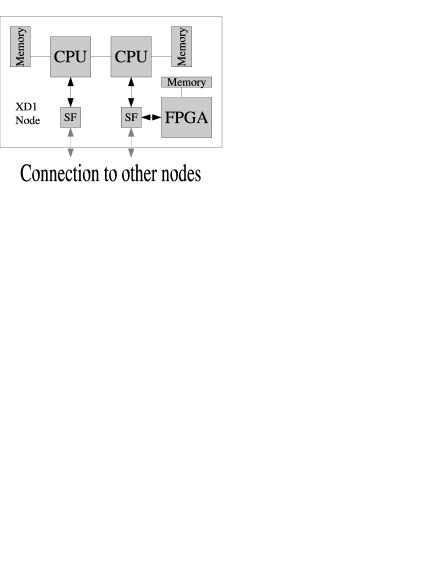
Figure 1: A diagram showing an overview of the Cray XD1 hardware. Six identical nodes containing two Opteron processors and an FPGA are connected via a high bandwidth interconnect. In the diagram, black arrows represent bi-directional data transfer at 3.2 GBs^-1 (1.6 GBs^-1 in each direction) and grey arrows represent bi-directional data transfer at 2 GBs^-1 (1 GBs^-1 in each direction). The memory is connected with a bandwidth of 12.8 GBs^-1 to the FPGA and 6.4 GBs^-1 to each CPU. The components labelled “SF” are the switching fabric processors. The FPGA is also connected directly to those in other nodes via high-bandwidth serial link.

The XD1 operating system is an optimised version of Suse Linux with improvements made by Cray [Brown, D. H., 2004]. The high bandwidth interconnect between nodes is designed for low latency communication, with MPI having a latency of only 1.6 $\mu$s and a sustainable bandwidth of 900 MB/s (in one direction) between nodes, as measured on the Durham system.

1.3 Programmable logic

Often software algorithms will consist of a simple repetitive task that is performed many times, thus requiring large amounts of CPU processing time. If this task can be offloaded from the CPU to some application accelerator, the CPU is then free to carry out other tasks, thus reducing the total time to complete a calculation. Programmable logic, in the form of an FPGA is ideal for use as an application accelerator. A simplistic view of an FPGA is that of a large amount of logic (AND, OR, NOT gates, latches, etc.) which can be connected in a user determined way. Logic can then be built up within the FPGA to perform simple (or even complicated) tasks.

An FPGA will normally be programmed using a hardware description language (HDL), such as VHDL. Once written by the user, code is synthesised and mapped into the FPGA. Common algorithms which can be placed into an FPGA include fast Fourier transforms (FFTs) and hardware control algorithms.

An FPGA will typically be clocked at only a tenth of the speed of a CPU. However, by implementing many operations in parallel, they can give a performance improvement due to the high degree of parallelisation that they afford. Fig. 2 shows a comparison of a pipeline implemented in an FPGA and a CPU, and demonstrates the parallelisation available to an FPGA user.

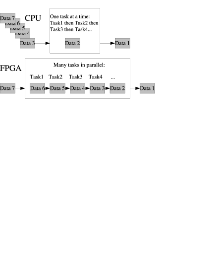
Figure 2: A diagram showing a comparison of a set of calculations performed in serial in a CPU and the same calculations implemented in a parallel pipeline in an FPGA. The CPU carries out tasks sequentially to a given piece of data. The FPGA carries out many tasks simultaneously on different pieces of data.

The XD1 supercomputer at Durham contains six FPGAs, each with 53, 136 logic cells. These can be used to help accelerate the AO simulations. Currently only the centroid algorithm, part of the Shack-Hartmann wavefront sensor (SHWFS) has been implemented in hardware and this is able to give a performance improvement when compared with an optimised software implementation. The FPGA clock speeds are user selectable, up to an absolute maximum of 199 MHz (set by Cray). The speed selected should be determined dependent on the user logic within the FPGA, and FPGA vendor tools such as ISE [Xilinx, 2005], give an estimate for the maximum clock speed that should be used with a given design and FPGA.

The results of the performance increases obtained from using the FPGAs are presented in the remainder of this paper, as are details of algorithms that will be implemented in hardware in the near future, along with estimates of the performance improvements these will give.

2 Hardware acceleration

As a first step we have implemented a centroid algorithm in the FPGAs. Although this is not the most demanding of applications for software, it maps well into hardware, and so is fairly straightforward to implement. This has allowed us to test interface code in the FPGA which is used to read and write data from and to the host CPU memory, develop a generic software interface to the FPGA and will also give us some idea of the performance gains which are attainable with the FPGA.

A SHWFS measures wavefront aberrations by measuring the wavefront gradient across the telescope aperture. This is done by dividing the aperture into a grid of sub-apertures using a lenslet array. The centroids of each sub-aperture image then represent the local wavefront slopes and this information can be used to shape the surface of a deformable mirror, thus removing or reducing the wavefront aberrations.

2.1 Centroid algorithm

The centroid algorithm that has been implemented in the FPGA reads sub-aperture image photon data from the host CPU main memory (requiring no CPU intervention), computes the $x$ and $y$ centroid positions of this sub-aperture and writes them back into the CPU main memory (again without CPU intervention). The sub-aperture image photon data is in the form of 16 bit unsigned integer numbers (typical of CCD pixel values), and the $x$ and $y$ centroid positions are returned in the form of 32 bit floating point numbers. These centroid positions are effectively the mean position of all the photons within the sub-aperture, and are computed within the FPGA by summing each individual photon count multiplied by its $x$ or $y$ position (in the range 0 to $N_{x,y}-1$ where $N_{x,y}$ represents the total number of pixels in the sub-aperture in the $x$ or $y$ direction), and dividing by the sum of all photons to give a fixed point number which is then converted into floating point. Finally, an offset equal to $\frac{N_{x,y}-1}{2}$ is subtracted from the $x$ and $y$ centroid position so that the numbers returned to the host CPU have a range from $-\frac{N_{x,y}-1}{2}$ to $\frac{N_{x,y}-1}{2}$ and a position of 0 represents the centre of the sub-aperture. This FPGA implementation gives an exact agreement with that obtained using a traditional software centroid algorithm.

2.1.1 User control

User application software is used to control the hardware centroid algorithm. The user can specify the start address to read sub-aperture image data from, and the number of bytes of data to read, as well as the address to which the $x$ and $y$ centroids should be written. The user is also able to specify the number of pixels in the $x$ and $y$ directions within the sub-aperture and to start and stop the centroid calculation. Additionally, the user can specify a pixel weighting, which will map a 16 bit input pixel value to a weighted pixel value to be used in the centroid algorithm. Two weightings commonly used are to raise the pixel values to the power of 1.5 or two.

This illustrates that although the FPGA is programmed with a fixed function, the user code that it implements can still be programmable. When programming an FPGA there is a trade-off between the flexibility of the algorithm and the time taken and FPGA resources used to implement the algorithm.

Once the centroid calculation has been started, the FPGA will read data from the specified memory bank in host memory, and whenever enough data has been read, will calculate a centroid value, which will be returned to the host memory. It is therefore possible to compute the centroid locations of many sub-apertures with a single start command.

2.2 Performance improvements

The performance of the FPGA when calculating centroids has been compared with that of optimised C code by comparing the time that each takes to compute centroids from data in an array of given size. This allows us to compare performance when accessing both large and small data arrays, and with different sized sup-apertures.

2.2.1 Processing time

Fig. 3 shows the time taken by the FPGA and C code to apply the centroid algorithm to a given amount of data. Timings for several different FPGA clock speeds are shown. The logic we have implemented allows us to operate the FPGA at speeds up to 199 MHz. However, we have also investigated performance at lower clock speeds because future developments may necessitate the use of lower clock speeds, for example if the simulation of CCD readout noise is implemented in the FPGA, and the logic is such that a slower clock speed is required.

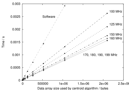
Figure 3: A diagram showing the time required to apply the centroid algorithm to a given amount of data. The performance of optimised C code (labelled software) running on the 2.2 GHz Opteron processors is shown along with the performance of the FPGA algorithm operating at different (labelled) clock speeds. The data to which the centroid algorithm is applied is composed of sub-apertures each with 16 pixels ($4\times 4$), with each pixel represented by 16 bits. The best fit lines are shown.

The gradient of the lines in Fig. 3 represent the time in seconds to apply the centroid algorithm to a given amount of data in bytes. The FPGA is able to transfer eight bytes of memory every clock cycle both into and out of the FPGA simultaneously, and due to the pipelined design of the FPGA centroid algorithm, data transfer should be the performance limiting factor. With a 100 MHz clock, the FPGA should be able to transfer data at a maximum rate of 800 MBs^-1, corresponding to 1.25 ns per byte. This is equal to the gradient of the 100 MHz data on the diagram, meaning that near maximum performance is being achieved, and that this performance is bandwidth limited as expected. Similarly, for clock speeds up to 170 MHz, we find that the theoretical data transfer rate is matched by the gradients on the diagram. However, at clock speeds above 170 MHz, the computation time does not decrease further.

A clock speed of 199 MHz should provide a maximum data transfer rate of 1592MBs^-1, corresponding to a data transfer time of about 0.625 ns per byte. However, as shown in Fig. 3, this is not achieved.

Fig. 4 shows the performance gained when implementing the centroid algorithm in hardware as a function of FPGA clock speed. The sharp cutoff at 170 MHz, corresponding to a data transfer rate of 1.36 GBs^-1 (8 bytes per clock cycle) occurs because this data transfer rate is approaching the theoretical maximum allowed between the CPU and FPGA (1.592 GBs^-1). The memory is accessed from the FPGA via the Opteron memory controller and a fabric switch (see Fig. 1), and these also have to arbitrate CPU access to the memory and communication between other computational nodes within the XD1 system, reducing performance below the theoretical maximum. This suggests that maximum data transfer performance (and hence centroid performance) can be achieved with a FPGA clock speed of 170 MHz. Increasing the clock speed above this will not give a performance increase, and the centroid data processing pipeline in the FPGA will be idle for some clock cycles when no new data has arrived from the memory.

Figure 4: A diagram showing the increase in performance when the centroid algorithm is computed in hardware instead of software as a function of FPGA clock speed, with the performance increase being the ratio of software computation time to hardware computation time. A sharp cutoff at 170 MHz shows the point at which the data bus is saturated. A total of 2 MB of sub-aperture pixel data was centroided, with 16 pixels per sub-aperture and 16 bits per pixel.

2.2.2 FPGA latencies

Fig. 5 shows the time taken to apply the centroid algorithm to a small amount of sub-aperture image photon data. The $y$ axis intercepts for the FPGA data are equal to about 3-5 $\mu$s dependent on clock speed, and this represents the latencies involved when using the FPGAs. A functional simulation of the FPGA algorithm (using tools provided by the FPGA vendor) shows that the time between the last data arriving in the FPGA and leaving the FPGA should be of order 2-3 $\mu$s (dependent on clock speed), due to the length of the FPGA algorithm pipeline. The additional 1-2 $\mu$s latency are due to the memory arbitration between the CPU and FPGA and time taken by software to start the FPGA operation.

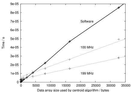
Figure 5: A diagram showing the time required to apply the centroid algorithm to a given amount of data, as with Fig. 3. The solid black curve represents the time taken by the software implementation while the grey lines represent the time taken by the FPGA implementation at 100 and 199 MHz. The grey lines are the same as those representing the same clock speed in Fig. 3.

Fig. 5 shows that when applying the centroid algorithm to less than about 2-4 KB data (depending on clock speed), it is faster to compute the centroids using the CPU, as the FPGA overheads then begin to dominate. However, in a typical AO simulation, a very large number of centroids will be computed.

2.2.3 Relative performance

The most important reason for using FPGAs in AO simulation is for the improved performance that they are able to give. Fig. 6 shows a comparison of the time taken to calculate centroid positions using the FPGA and when using C code.

When using FPGA clock speeds above 170 MHz, the centroid algorithm is up to four times faster in the FPGA when compared to the C algorithm for memory blocks greater than about 100 KB. For smaller memory blocks, the latency introduced when using the FPGA begins to have a larger effect and so the performance gain reduces. However, even when using a 4 KB memory block (two $32\times 32$ pixel sub-apertures or 128 $4\times 4$ pixel sub-apertures at 16 bits per pixel), the FPGA still gives some performance gain with the software algorithm taking almost twice as long to perform the same computation.

Figure 6: A diagram showing the increase in performance seen when using an FPGA centroid algorithm instead of a software algorithm. The performance gain is seen to level out when the centroid algorithm is applied to more than about 100 KB of sub-aperture pixel data. The performance increase is defined as the ratio of the time taken by software to the time taken by hardware when applying the centroid algorithm. The data to which the centroid algorithm is applied is composed of sub-apertures each with 16 pixels, with each pixel represented by 16 bits.

When applying the centroid algorithm to a dataset of a given size, the performance of the software algorithm will depend partly on the number of pixels in each sub-aperture, as shown in Fig. 7. However, the FPGA implementation does not have this dependence, since the pipeline architecture is independent of the sub-aperture size, with computation time depending only on the total amount of data and the small fixed pipeline latency.

Figure 7: A diagram showing the effect of sub-aperture size on centroid computation time for the software algorithm (dashed curve) and the hardware algorithm (solid line). A total of 2 MB data were input to the centroid algorithm in this case (1 MPixels).

3 Future considerations and improvements

The performance increase of four times when using the FPGAs may seem small, particularly when considering the amount of time required to write and debug the VHDL code for the FPGA. A flexible software centroid algorithm can be written in C taking only 10–20 lines of code. However, when implemented in hardware, our implementation contains about 2000 lines of code for host memory access (reading pixel values from host CPU memory, and writing the centroid values to host memory) and about 1200 lines of code for the centroid algorithm (of which half of this is responsible for fixed point to floating point conversion and pipeline flow control). This does not include the libraries used, which are treated as black boxes (for example Cray specific libraries, division libraries, and FPGA block memory access libraries), and for which, there is no source code available.

However, only about a quarter of the FPGA has been used (a large fraction of which is the logic to read and write data from and to the CPU memory), and there is therefore room for extra logic to perform additional calculations. If these additional calculations are able to act on the data immediately before or after the centroid algorithm, they will take virtually no extra time to compute, since the limiting factor is the time taken to read data into and out of the FPGA. The performance gained over software implementations will therefore be much greater, depending on the amount of calculation transferred into the FPGA pipeline.

3.1 Pipeline extensions

The current success of the FPGA algorithm is thus only the start of the hardware acceleration that can be achieved using the FPGAs and is limited by the rate at which data can be passed into and out of the FPGA. We aim to extend the number of algorithms that are placed within the hardware, including the algorithms related to the Monte-Carlo nature of the simulation. By ensuring that these algorithms are part of a single SHWFS pipeline, data transfers to and from host memory can be minimised, thus maximising the performance of the FPGA algorithms. The initial aim is to implement an AO simulation pipeline as shown in Fig. 8. This includes a 2D FFT of the input optical complex amplitude, high light level PSF computation (by taking the squared modulus of the output of the 2D FFT algorithm), the inclusion of sky background noise, photon shot noise, CCD readout noise, noise and background subtraction and finally the centroid algorithm. With such a pipeline, atmospheric pupil phase data will be read into the pipeline by the FPGA, and the centroid values will be written back to the host CPU memory. Due to the highly parallel nature of FPGAs, the total computation time will be virtually identical to that presented for the centroid algorithm here, with a slightly higher initial latency (which is negligible when large amounts of data are involved). To perform such a pipeline in software takes much longer as each stage would be performed in series, with the total computation time being the sum of the times for each individual stage.

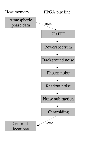
Figure 8: A diagram showing the pipeline stages which will eventually be implemented in the FPGA logic. Data will be read into the FPGA at the start of the pipeline, and the result transferred back to the host CPU at the end of the pipeline.

3.2 Expected pipeline performance

Once the pipeline shown in Fig. 8 has been implemented, the time to perform these calculations in the FPGA will be slightly greater than the times shown in Fig. 3, due to a slight increase (of order microseconds) in the initial latency due to the longer pipeline. When considering the simulation of an AO system with $32\times 32$ sub-apertures each with $8\times 8$ atmospheric complex amplitude values (32 bit floating point), a total of $32^{2}\times 8^{2}\times 4=262144$ bytes will need to be read into the FPGA, which with a 170 MHz clock will take approximately 200 $\mu$s. The current software simulation can perform this operation in approximately 0.25 s and so the performance will be increased by up to 1000 times, an improvement which would be difficult and expensive to achieve using only CPU based solutions.

3.3 Separate algorithms

In addition to implementing the pipeline in Fig. 2 in hardware, we also intend to implement several other algorithms in the FPGA:

1. Atmospheric phase screen generation

2. Wavefront reconstructor algorithms

3. Deformable mirror surface figure calculations

4. Science PSF calculation

These algorithms will help to improve the performance of the AO simulations further. Since they will not be integrated into the SHWFS pipeline, they must operate separately from the SHWFS pipeline and so may be placed in different FPGAs, thus having certain nodes of the XD1 dedicated to certain parts of the AO simulation.

4 Conclusion

We have presented an overview of initial performance improvements made to the Durham AO simulation platform using programmable logic (FPGAs). At present, only a centroid algorithm has been implemented in hardware, and this gives performance improvements of up to a factor of four when compared to optimised C algorithms. By implementing more of the simulation in the FPGA we expect to increase the speed of AO simulation by up to 1000 times. In this way we expect to implement realistic simulations of ELT-scale AO systems on a single Cray XD1 platform, at speeds that will be useful for detailed design and optimisation studies of future instruments.

References

- Ahmadia and Ellerbroek [2003] A. J. Ahmadia and B. L. Ellerbroek. Parallelized simulation code for multiconjugate adaptive optics. In Astronomical Adaptive Optics Systems and Applications. Edited by Tyson, Robert K.; Lloyd-Hart, Michael. Proceedings of the SPIE, Volume 5169, pp. 218-227 (2003)., pages 218–227, December 2003.
- Brown, D. H. [2004] Brown, D. H. Cray XD1 brings high-bandwidth supercomputing to the mid-market. Technical report, D. H. Brown Associates, Inc., http://www.cray.com/products/xd1/resources, October 2004.
- Carbillet et al. [2005] M. Carbillet, C. Vérinaud, B. Femenía, A. Riccardi, and L. Fini. Modelling astronomical adaptive optics - I. The software package CAOS. MNRAS, 356:1263–1275, February 2005.
- Conan et al. [2003] R. Conan, M. Le Louarn, J. Braud, E. Fedrigo, and N. N. Hubin. Results of AO simulations for ELTs. In Future Giant Telescopes. Edited by Angel, J. Roger P.; Gilmozzi, Roberto. Proceedings of the SPIE, Volume 4840, pp. 393-403 (2003)., pages 393–403, January 2003.
- Cray [2005] Cray. Cray XD1 Supercomputer. Cray, http://www.cray.com/products/xd1/, 1.3 edition, 2005.
- Doel [1995] A. P. Doel. Comparison of Shack-Hartmann and curvature sensing for large telescopes. In Proc. SPIE Vol. 2534, p. 265-276, Adaptive Optical Systems and Applications, Robert K. Tyson; Robert Q. Fugate; Eds., pages 265–276, August 1995.
- Gendron et al. [2004] E. Gendron, A. Coustenis, P. Drossart, M. Combes, M. Hirtzig, F. Lacombe, D. Rouan, C. Collin, S. Pau, A.-M. Lagrange, D. Mouillet, P. Rabou, T. Fusco, and G. Zins. VLT/NACO adaptive optics imaging of Titan. A&A, 417:L21–L24, April 2004.
- Le Louarn et al. [2004] M. Le Louarn, C. Verinaud, V. Korkiakoski, and E. Fedrigo. Parallel simulation tools for AO on ELTs. In Advancements in Adaptive Optics. Edited by Domenico B. Calia, Brent L. Ellerbroek, and Roberto Ragazzoni. Proceedings of the SPIE, Volume 5490, pp. 705-712 (2004)., pages 705–712, October 2004.
- Marchetti et al. [2004] E. Marchetti, R. Brast, B. Delabre, R. Donaldson, E. Fedrigo, C. Frank, N. N. Hubin, J. Kolb, M. Le Louarn, J. Lizon, S. Oberti, R. Reiss, J. Santos, S. Tordo, R. Ragazzoni, C. Arcidiacono, A. Baruffolo, E. Diolaiti, J. Farinato, and E. Vernet-Viard. MAD status report. In Advancements in Adaptive Optics. Edited by Domenico B. Calia, Brent L. Ellerbroek, and Roberto Ragazzoni. Proceedings of the SPIE, Volume 5490, pp. 236-247 (2004)., pages 236–247, October 2004.
- Masciadri et al. [2005] E. Masciadri, R. Mundt, T. Henning, C. Alvarez, and D. Barrado y Navascués. A Search for Hot Massive Extrasolar Planets around Nearby Young Stars with the Adaptive Optics System NACO. Ap.J., 625:1004–1018, June 2005.
- Mouillet et al. [2004] D. Mouillet, A. M. Lagrange, J.-L. Beuzit, C. Moutou, M. Saisse, M. Ferrari, T. Fusco, and A. Boccaletti. High Contrast Imaging from the Ground: VLT/Planet Finder. In ASP Conf. Ser. 321: Extrasolar Planets: Today and Tomorrow, pages 39–+, December 2004.
- Russell et al. [2004] A. P. G. Russell, T. G. Hawarden, E. Atad-Ettedgui, S. K. Ramsay-Howat, A. Quirrenbach, R. Bacon, and R. M. Redfern. Instrumentation studies for a European extremely large telescope: a strawman instrument suite and implications for telescope design. In Emerging Optoelectronic Applications. Edited by Jabbour, Ghassan E.; Rantala, Juha T. Proceedings of the SPIE, Volume 5382, pp. 684-698 (2004)., pages 684–698, July 2004.
- Vérinaud et al. [2005] C. Vérinaud, M. Le Louarn, V. Korkiakoski, and M. Carbillet. Adaptive optics for high-contrast imaging: pyramid sensor versus spatially filtered Shack-Hartmann sensor. MNRAS, 357:L26–L30, February 2005.
- Xilinx [2005] Xilinx. ISE data sheet. Xilinx, http://www.xilinx.com/ise, 7 edition, 2005.