An X-ray emission line spectrum of Nova V382 Velorum 1999

Abstract

We report on the analysis of an X-ray grating spectrum of the Classical Nova V382 Vel (1999), obtained with the LETG+HRC-S instrument on board CHANDRA, which shows emission lines dominating over any continuum. Lines of Si, Mg, Ne, O, N, and C are identified, but no Fe lines are detected. The total luminosity in the lines is $\sim 4\times 10^{27}$ erg s^-1 (corrected for N${}_{\rm H}=1.2\times 10^{21}$ cm^-2). The lines have broad profiles with FWHM corresponding to a velocity $\sim 2900\,\pm\,200$ km s^-1. Some structure is identified in the profiles, but for different elements we find different profile structures. While lines of O show a broadened Gaussian profile, those of Ne are double-peaked, suggesting a fragmented emitting plasma. Using the emission measure distribution we derive relative element abundances and find abundances of Ne and N that are significantly enhanced relative to that of O, while Fe is not over-abundant. The lack of any source emission longwards of 50 Å and the O viii Ly_α/Ly_β line ratio support previous values of the hydrogen column-density. We find weak continuum emission from the white dwarf, consistent with a black-body spectrum with an upper limit to the temperature of $T=3\times 10^{5}$ K, assuming a source radius of 6000 km. The upper limit for the integrated black-body luminosity is $2\times 10^{36}$ erg s^-1. The BeppoSAX and Chandra ACIS observations of V382 Vel show that the nova was bright and in the Super Soft phase as late as 1999 December 30. Our LETG observation obtained 6 weeks later, as well as all subsequent X-ray observations, showed a remarkable fading to a nearly pure emission line phase which suggests that nuclear burning on the white dwarf had turned off by February. In the absence of a photoionizing source the emission lines were formed in a collisionally ionized and excited expanding shell.

1 Introduction

Classical Novae (CN), a class of Cataclysmic Variables (CVs), are thought to be thermonuclear explosions induced on the surface of white dwarfs as a result of continuous accretion of material from a companion main sequence star. A sufficient accumulation of hydrogen-rich fuel causes a thermonuclear runaway (TNR). Extensive modelling of the TNR has been carried out in the past (e.g., Starrfield, 1989, and references therein). These models showed that only a part of the ejected envelope actually escapes, while the remaining material forms an envelope on the white dwarf with ongoing nuclear burning, radiation driven winds, and turbulent motions. These processes result in a shrinking of the nuclear burning white dwarf radius with increasing temperatures (Starrfield et al., 1991; Krautter, 2002). During this phase of “constant bolometric luminosity” the nova emits strong X-ray radiation with a soft spectral signature.
Classical Novae have been observed with past X-ray missions, e.g., Einstein, ROSAT, ASCA, and BeppoSAX. While X-ray lightcurve variations were studied, the X-ray spectra obtained had low dispersion and were quite limited. The transmission and reflection gratings aboard Chandra and XMM-Newton now provide significantly improved sensitivity and spectral resolution, and these gratings are capable of resolving individual emission or absorption lines. The Chandra LETG (Low Energy Transmission Grating) spectrum of the Classical Nova V4743 Sgr (Ness et al., 2003) showed strong continuum emission with superimposed absorption lines, while V1494 Aql showed both absorption and emission lines (Drake et al., 2003). Essentially all X-ray spectra of Classical Novae differ from each other, so no classification scheme has so far been established. A review of X-ray observations of novae is given by Orio (2004).

Table 1: Summary of X-ray, UV and optical observations of V382 Vel

Date	day after outburst	Mission	Remarks	Reference
	5–498	La Silla	$V_{\rm max}=2.3$ (1999 23 May)	Della Valle et al. (2002)
			fast Ne Nova; d=1.7 kpc ($\pm 20$ per cent)
1999 May 26	5.7	RXTE	faint in X-rays	Mukai & Ishida (2001)
1999 June 7	15	BeppoSAX	first X-ray detection	Orio et al. (2001)
			no soft component
1999 June 9/10	20.5	ASCA	highly absorbed bremsstrahlung	Mukai & Ishida (2001)
1999 June 20	31	RXTE	decreasing plasma temperature	Mukai & Ishida (2001)
1999 June 24	35	RXTE	and column-density	Mukai & Ishida (2001)
1999 July 9	50	RXTE	$\stackrel{{\scriptstyle.}}{{.}}$	Mukai & Ishida (2001)
1999 July 18	59	RXTE	$\stackrel{{\scriptstyle.}}{{.}}$	Mukai & Ishida (2001)
1999 May 31–		HST/STIS	UV lines indicate fragmentation of	Shore et al. (2003)
1999 Aug 29			ejecta;
			C and Si under-abundant,
			O, N, Ne, Al over-abundant
			$d=2.5$ kpc; N${}_{\rm H}=1.2\times 10^{21}$ cm-2
1999 Nov 23	185	BeppoSAX	hard and soft component	Orio et al. (2001, 2002)
1999 Dec 30	223	Chandra (ACIS)		Burwitz et al. (2002)
2000 Feb 6– Jul 3		FUSE	O vi line profile	Shore et al. (2003)
2000 Feb 14	268	Chandra (LETG)	details in this paper	Burwitz et al. (2002)
2000 Apr 21	335	Chandra (ACIS)		Burwitz et al. (2002)
2000 Aug 14	450	Chandra (ACIS)		Burwitz et al. (2002)

2 The Nova

2.1 V382 Velorum

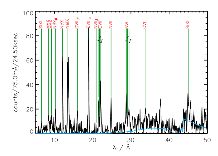
Figure 1: Chandra LETG spectrum of V382 Vel (background subtracted). Only emission lines can be seen with some weak continuum between 30 and 40 Å. A diluted ($R=6000$ km, $d=2.5$ kpc) thermal black-body spectrum (absorbed by $N_{\rm H}=1.2\times 10^{21}$ cm^-2) is overplotted on the spectrum and suggests that the weak continuum is emission from the underlying white dwarf. The temperature used for the source is $T=3\times 10^{5}$ K implying a luminosity of $2\times 10^{36}$ erg s^-1.

The outburst of the Classical Nova V382 Vel was discovered on 1999 May 22 (Gilmore, 1999). V382 Vel reached a $V_{\rm max}$ brighter than 3, making it the brightest nova since V1500 Cyg in 1975. Della Valle et al. (2002) described optical observations of V382 Vel and classified the nova as fast and belonging to the Fe ii broad spectroscopic class. Its distance was estimated to be $1.7\,\pm\,0.34$ kpc. Infrared observations detected the [Ne ii] emission line at 12.8 $\mu$m characteristic of the “neon nova” group and, subsequently, V382 Vel was recognized as an ONeMg nova (Woodward et al., 1999). An extensive study of the ultraviolet (UV) spectrum was presented by Shore et al. (2003), who analysed spectra obtained with the Space Telescope Imaging Spectrograph (STIS) on the Hubble Space Telescope (HST) in 1999 August as well as spectra from the Far Ultraviolet Spectroscopic Explorer (FUSE). They found a remarkable resemblance of Nova V382 Vel to V1974 Cyg (1992), thus imposing important constraints on any model for the nova phenomenon.
Following an “iron curtain” phase (where a significant fraction of the ultraviolet light is absorbed by elements with atomic numbers around 26) V382 Vel proceeded through a stage when P Cygni line profiles were detected for all important UV resonance lines (Shore et al., 2003). The line profiles displayed considerable sub-structure, indicative of fragmentation of the ejecta at the earliest stages of the outburst. The fits to the UV spectra suggested a distance of 2.5 kpc, higher than the value given by Della Valle et al. (2002). From the spectral models, Shore et al. (2003) were able to determine element abundances for He, C, N, O, Ne, Mg, Al, and Si, relative to solar values. While C and Si were found to be under-abundant, O, Ne, and Al were significantly over-abundant compared to solar values. From the H Ly_α line at 1216 Å, Shore et al. (2003) estimated a value for the hydrogen column-density of $N_{\rm H}=1.2\times 10^{21}$ cm^-2.

2.2 Previous X-ray observations of V382 Vel

Early X-ray observations of V382 Vel were carried out with the RXTE on day 5.7 by Mukai & Swank (1999), who did not detect any significant X-ray flux (see Table 1). X-rays were first detected from this nova by BeppoSAX on day 15 (cf., Orio et al., 2001) in a very broad band from 0.1–300 keV. A hard spectrum was found between 2 and 10 keV which these authors attributed to emission from shocked nebular ejecta at a plasma temperature $kT_{e}\,\sim\,6$ keV. No soft component was present in the spectrum. On day 20.5 Mukai & Ishida (2001) found, from ASCA observations, a highly absorbed ($N_{\rm H}\sim$ 10²³ cm^-2) bremsstrahlung spectrum with a temperature $kT_{e}\sim 10$ keV. In subsequent observations with RXTE (days 31, 35, 50, and 59) the spectrum softened because of decreasing temperatures ($kT_{e}\sim 4.0$ keV to $kT_{e}\sim 2.4$ keV on day 59) and diminishing $N_{\rm H}$ ($7.7\times 10^{22}$ cm^-2 on day 31 to $1.7\times 10^{22}$ cm^-2 on day 59). Mukai & Ishida (2001) argued that the X-ray emission arose from shocks internal to the nova ejecta. Like Orio et al. (2001), they did not find any soft component. Six months later, on 1999 November 23, Orio et al. (2002) obtained a second BeppoSAX observation and detected both a hard component and an extremely bright Super-Soft component. By that time the (absorption-corrected) flux of the hard component (0.8–2.4 keV) had decreased by about a factor of 40, however, the flux below $\sim 2$ keV increased by a larger factor (Orio et al., 2002).

Chandra Target of Opportunity (ToO) observations were reported by Burwitz et al. (2002). These authors used both ACIS and the LETG to observe V382 Vel four times and they gave an initial analysis of the data obtained. The first ACIS-I observation was obtained on 1999 December 30 and showed that the nova was still in the Super Soft phase (as seen by Orio et al., 2002, about 2 months before) and was bright. This observation was followed on 2000 February 14 by the first high-resolution X-ray observation of any nova in outburst, using the Low Energy Transmission Grating (LETG+HRC-S) on board Chandra. Its spectral resolution of R$\sim$600 surpasses the spectral resolution of the other X-ray detectors by factors of up to more than two orders of magnitude.
We found that the strong component at $\sim 0.5$ keV had decreased significantly and was replaced by a (mostly) emission line spectrum above 0.7keV. The total flux observed in the 0.4–0.8 keV range had also declined by a factor of about 100 (Burwitz et al., 2002). The grating observation was followed by two more ACIS-I observations (2000 April 21 and August 14) which showed emission lines and a gradual fading after the February observation. We therefore conclude that the hydrogen burning on the surface of the white dwarf in V382 Vel must have turned off sometime between 1999 December 30 and 2000 February 14, resulting in a total duration of 7.5–8 months for the TNR phase. This indicates that the white dwarf in V382 Vel has a high mass which is consistent with its ONeMg nature and short decay time, t₃ (Krautter et al., 1996). We speculate that hydrogen burning turned off shortly after the 1999 December 30 observation, since a cooling time of less than 6 weeks seems extremely short (Krautter et al., 1996).
In this paper we analyse the Chandra LETG spectrum obtained on 2000 February 14 and present a detailed description of the emission line spectrum. We describe our measurements and analysis methods in Section 3. Our results are given in Section 4, where we discuss interstellar hydrogen absorption, line profiles, the lack of iron lines and line identifications. Our conclusions are summarized in Sections 5 and 6.

3 Analysis

The V382 Velorum observation was carried out on 2000 February 14, 06:23:10 UT with an exposure time of 24.5 ksec. We extracted the Chandra LETG data from the Chandra archive and analysed the preprocessed pha2 file. We calculated effective areas with the $fullgarf$ task provided by the CIAO software. The background-subtracted spectrum is shown in Fig. 1. It shows emission lines but no strong continuum emission. For the measurement of line fluxes we use the original, non-background-subtracted spectrum. The instrumental background is instead added to a model spectrum constructed from the spectral model parameters – wavelengths, line widths, and line counts. The spectral model consists of the sum of normalized Gaussian line profiles, one for each emission line, which are each multiplied by the parameter representing the line counts. Adding the instrumental background to the spectral model is equivalent to subtracting the background from the original spectrum (with the assumption that the background is the same under the source as it was measured adjacent to the source), but is necessary in order to apply the Maximum Likelihood method conserving Poisson statistics as required by Cash (1979) and implemented in Cora (Ness & Wichmann, 2002). We also extracted nine LETG spectra of Capella, a coronal source with strong emission lines, which are purely instrumentally broadened (e.g., Ness et al., 2001; Ness et al., 2003). The combined Capella spectrum is used as a reference in order to detect line shifts and anomalies in line widths in the spectrum of V382 Vel. Previous analyses of Capella (e.g., Argiroffi et al., 2003) have shown that the lines observed with Chandra are at their rest wavelengths.

For the measurement of line fluxes and line widths we use the Cora program (Ness & Wichmann, 2002). This program is a maximum likelihood estimator providing a statistically correct method to treat low-count spectra with less than 15 counts per bin. The normal $\chi^{2}$ fitting approach requires the spectrum to be rebinned in advance of the analysis in order to contain at least 15 counts in each spectral bin, thus sacrificing spectral resolution information. Since background subtraction results in non-Poissonian statistics, the model spectrum, $c_{i}$, consists of the sum of the background spectrum, $BG$ (instrumental background plus an a priori given constant source continuum), and $N_{L}$ spectral lines, represented by a profile function $g_{i,j}(\lambda,\sigma)$. Then

$$c_{i}=BG+\sum^{N_{L}}_{j=0}A_{j}\cdot g_{i,j}(\lambda,\sigma)$$ (1)

with $A_{j}$ the number of counts in the $j$-th line. The formalism of the Cora program is based on minimizing the (negative) likelihood function

$${\cal L}=-2\ \ln P=-2\sum_{i=1}^{N}(-c_{i}+n_{i}\ln c_{i})$$ (2)

with $n_{i}$ being the measured (non-subtracted) count spectrum, and $N$ the number of spectral bins. We model the emission lines as Gaussians representing only instrumentally broadened emission lines in the case of the coronal source Capella (e.g., Ness et al., 2001). In V382 Vel the lines are Doppler broadened, but, as will be discussed in Section 4.3, we have no reason to use more refined profiles to fit the emission lines in our spectrum. The Cora program fits individual lines under the assumption of a locally constant underlying source continuum. For our purposes we set this continuum value to zero for all fits, and account for the continuum emission between 30 and 40 Å by adding the model flux to the instrumental background. All line fluxes are then measured above the continuum value at the respective wavelength (see Fig. 1).

4 Results

4.1 Interstellar absorption

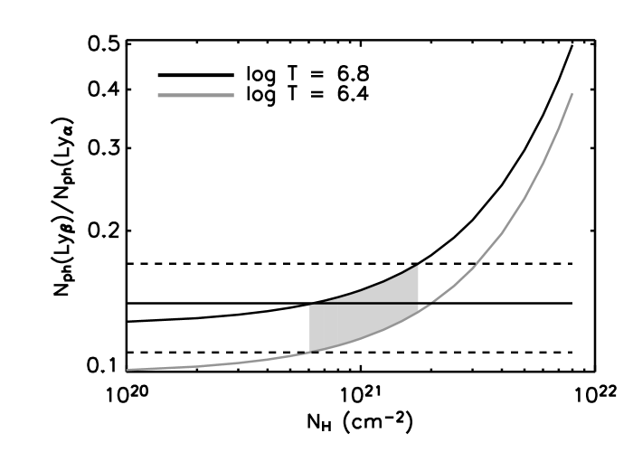
Figure 2: Dependence of the photon flux ratio for O viii Ly_β/Ly_α on $N_{\rm H}$. As $N_{\rm H}$ increases, Ly_α is more absorbed than Ly_β. The grey shaded area marks the range of $N_{\rm H}$ consistent with our measurement of O viii Ly_β/Ly_α, with associated errors.

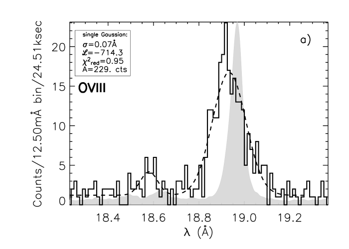
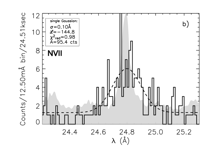
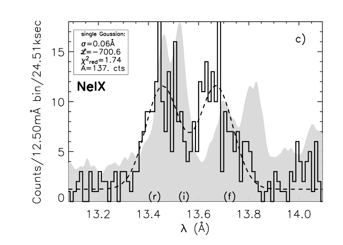
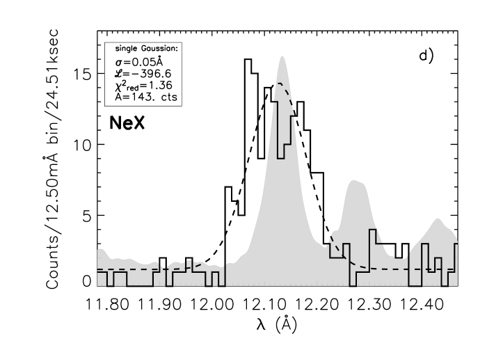
Figure 3: Profile analysis of the strongest, isolated lines. Best-fitting profiles using a single, broadened Gaussian line template are also shown. The light curves are arbitrarily scaled smoothed LETG spectra of Capella representing the instrumental resolving power. The legend gives the fit parameters, where $sigma$ is the line width, $\ell$ is the best likelihood value, $\chi^{2}$ a goodness parameter and A the number of counts in the lines.

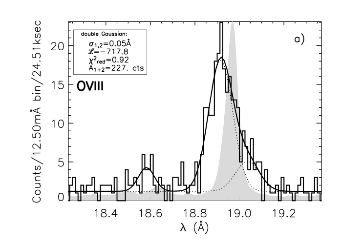
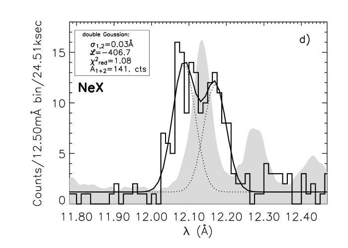
Figure 4: Profile analysis of the strongest, isolated lines. The best-fitting profiles using two instrumentally broadened Gaussian lines (dotted lines mark the individual components) can be compared with Fig. 3. The fit parameters are defined in the caption of Fig. 3.

Since V382 Vel is located at a considerable distance along the Galactic plane, substantial interstellar absorption is expected to affect its soft X-ray spectra. In the early phases, spectral fits to RXTE and ASCA data taken immediately after the outburst (1999 May 26 to July 18) showed a decrease of $N_{\rm H}$ from $10^{23}$ cm^-2 to $<5.1\times 10^{22}$ cm^-2 (Mukai & Ishida, 2001). BeppoSAX observations carried out in 1999 November revealed an $N_{\rm H}$ around $2\times 10^{21}$ cm^-2 (Orio et al., 2002). In 1999 August, the expanding shell was already transparent to UV emission and Shore et al. (2003) measured an $N_{\rm H}$ of $1.2\times 10^{21}$ cm^-2.

The high-resolution X-ray spectrum offers a new opportunity to determine $N_{\rm H}$ from the observed ratio of the O viii Ly_α and Ly_β line fluxes. This line ratio depends only weakly on temperature, but quite sensitively on $N_{\rm H}$ (see Fig. 2). From the photon flux ratio of 0.14 $\pm$ 0.03 (which has been corrected for the effective area), we infer an equivalent $N_{\rm H}$-column-density between $6\times 10^{20}$ cm^-2 (assuming $\log T=6.4$) and $2\times 10^{21}$ cm^-2 (assuming $\log T=6.8$), which is consistent with the value determined by Shore et al. (2003). This value appears to represent the true interstellar absorption, rather than absorption intrinsic to the nova itself. For our spectral analyses we adopt this value and calculate transmission coefficients from photoelectric absorption cross-sections using the polynomial fit coefficients determined by Balucinska-Church & McCammon (1992). We assume standard cosmic abundances from Anders & Grevesse (1989) as implemented in the software package PINTofALE (Kashyap & Drake, 2000).

4.2 Continuum emission

All previous X-ray spectra of V382 Vel were probably dominated by continuum emission although we cannot rule out the possibility that the continuum consisted of a large number of overlapping emission lines. In contrast, the LETG spectrum from 2000 Feb 14 does not exhibit continuum emission over the entire wavelength range. However, some ’bumps’ can be seen in Fig. 1 at around 35 Å, which could be interpreted as weak continuum emission, or could be the result of a large number of weak overlapping lines. The low count rate around 44 Å is due to C absorption in the UV shield, filter and detector coating at this wavelength. We calculated a diluted thermal black-body spectrum for the WD, absorbed with $N_{\rm H}=1.2\times 10^{21}$ cm^-2 (Section 4.1). The continuum is calculated assuming a WD radius of 6000 km, a distance of 2.5 kpc and a temperature of $3\times 10^{5}$ K. Given the possible presence of weak lines, this temperature is an upper limit. The intrinsic (integrated) luminosity implied by the black-body source is $L_{\rm BB}=2\times 10^{36}$ erg s^-1 (which corresponds to an X-ray luminosity of $\sim 10^{28}$ erg s^-1. The black-body spectrum was then multiplied by the exposure time and the effective areas in order to compare it with the (rebinned) count spectrum shown in Fig. 1. We do not use the parameters of the black-body source in our further analysis, but it is clear that even the highest possible level of continuum emission is not strong enough to excite lines by photoexcitation. Also, no high-energy photons are observed that could provide any significant photoexcitation or photoionization. In the further analysis, we therefore assume that the lines are exclusively produced by collisional ionization and excitation. We point out that, given the uncertainty in the assumed radius and distance, our upper limit to the black-body temperature is still consistent with the lower limit of $2.3\times 10^{5}$ K found by Orio et al. (2002) by fitting WD NLTE atmospheric models to the spectrum obtained in the second BeppoSAX observation.

4.3 Analysis of line properties

In Fig. 3, we show the spectral ranges around the strong resonance lines of the H-like ions O viii at 18.97 Å, N vii at 24.78 Å, and Ne x at 12.13 Å, the resonance line of the He-like ion Ne ix at 13.45 Å and the Ne ix forbidden line at 13.7 Å. In order to illustrate the instrumental line profile, we plot an LETG spectrum of Capella in a lighter shade (the Capella spectrum is arbitrarily scaled to give overall intensities that can be plotted on the same scales as those for Nova V382 Vel). Clearly, the lines in V382 Vel are significantly broadened compared to the emission lines in the Capella spectrum. We test two hypotheses to describe the broadening of the lines. First, we use a single Gaussian with an adjustable Gaussian line width parameter $\sigma$ (defined through $I=I_{0}e^{-0.5(\lambda-\lambda_{0})^{2}/\sigma^{2}}$). Secondly, we use a double Gaussian line profile with adjustable wavelengths. We show the best-fitting curves of single profiles in Fig. 3 and those of double profiles in Fig. 4 (individual components are dotted). For O viii, we also fit the N vii Ly_β line at 18.6 Å with a single Gaussian. In the legends we provide the goodness parameters ${\cal L}$ from equation 2 and $\chi^{2}$, which is only given for information, because it gives a quantitative figure of the quality of agreement, while the likelihood value ${\cal L}$ is only a relative number. To obtain the best fit we minimized ${\cal L}$, since our spectrum contains fewer than 15 counts in most bins, and $\chi^{2}$ does not qualify as a goodness criterion (Cash, 1979). The fit parameters, line width, $\sigma$, and line counts, $A$, are also given. For all fits, those models with two Gaussian lines return slightly better likelihood values. For O viii and N vii each component of the double Gaussian is broader than the instrumental line width indicating that the O viii and N vii emission originates from at least three different emission regions supporting the fragmentation scenario suggested by Shore et al. (2003). The O viii line appears blue-shifted with respect to the rest wavelengths with only weak red-shifted O viii emission. The N vii line is split into several weaker components around the central line position, indicating the highest degree of fragmentation, although the noise level is also higher. At longer wavelengths, fragmentation in velocity space can be better resolved owing to the increasing spectral resolution. The lines from both Ne x and Ne ix seem to be confined to two distinctive fragmentation regions. For other elements, this exercise cannot be carried out because the respective lines are too faint. From the Gaussian line widths of the single-line fits, converted to FWHM, we derive Doppler velocities and find 2600 km s^-1, 2800 km s^-1, 2900 km s^-1, and 3100 km s^-1 for O viii, N vii, Ne x, and Ne ix, respectively. These are roughly consistent within the errors ($\sim 200$ km s^-1) but they are lower than the expansion velocities reported by Shore et al. (2003), who found $4000$ km s^-1 (FWHM) from several UV emission lines measured some eight months earlier. What may be happening is that the density and emissivity of the fastest moving material is decreasing rapidly so that over time we see through it to slower, higher-density inner regions.

Fig. 5 shows a comparison of the profiles of the O viii and Ne x lines in velocity space ($v=c(\lambda-\lambda_{0})/\lambda_{0}$) with $\lambda_{0}=18.97$ Å for O viii and $\lambda_{0}=12.13$ Å for Ne x. The shaded O viii line is blue shifted, while Ne x shows a red-shifted and a blue-shifted component of more equal intensity at roughly similar velocities. In order to quantitatively assess the agreement between the two profiles we attempted to adjust the single-line profile of the O viii line (Fig. 3a) to the Ne x line, but found unsatisfactory agreement. We adjusted only the number of counts but not the wavelength or line width of the O viii template. The difference in $\chi^{2}$ given in the upper right legend clearly shows that the profiles are different. This can be due either to different velocity structures in the respective elements or to different opacities in the lines. In the latter case the red-shifted component of O viii would have to be absorbed while the plasma in the line-of-sight remained transparent to the red-shifted component of Ne x.

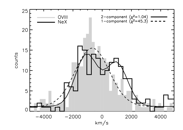
Figure 5: Direct comparison of velocity structure in O viii (light shade) and Ne x (dark line). The best-fitting double-line profile from Fig. 4c (solid) is compared to the rescaled single-line profile of Fig. 3a (dashed).

4.4 Line identifications

Table 2: Line fluxes (not corrected for N_H) detected in the LETG spectrum of V382 Vel with identifications using APEC (exposure time $\Delta$t=24.5 ksec)

$\lambda$	$\sigma^{[a]}$	line flux[b]	Aeff	$\lambda^{[c]}$	log($T_{M}^{[d]}$)	ID
(Å)	(Å)		(cm2)	(Å)	MK
6.65	0.06	4.79 $\pm$ 1.80	44.26	6.65	7.0	Si xiii (Her)
				6.74	7.0	Si xiii (Hef)
8.45	0.10	12.0 $\pm$ 2.50	37.98	8.42	7.0	Mg xii (Lyα)
9.09	0.04	6.68 $\pm$ 1.85	32.27	9.17	6.8	Mg xi (Her)
9.30	0.04	6.13 $\pm$ 1.72	32.27	9.31	6.8	Mg xi (Hef)
10.24	0.04	8.93 $\pm$ 1.99	28.62	10.24	6.8	Ne x (Lyβ)
12.12	0.05	31.4 $\pm$ 2.98	28.68	12.13	6.8	Ne x (Lyα)
13.45	0.05	24.7 $\pm$ 2.58	29.37	13.45	6.6	Ne ix (Her)
13.66	0.07	27.6 $\pm$ 2.72	29.42	13.70	6.6	Ne ix (Hef)
15.15	0.05	3.13 $\pm$ 1.14	30.37	15.18	6.5	O viii (Lyγ)
15.98	0.06	7.22 $\pm$ 1.45	29.98	16.01	6.5	O viii (Lyβ)
18.58	0.07	4.63 $\pm$ 1.23	26.16	18.63	6.3	O vii (1$\rightarrow$13)
18.93	0.07	36.0 $\pm$ 2.60	26.61	18.97	6.5	O viii (Lyα)
20.86	0.06	2.89 $\pm$ 1.32	17.33	20.91	6.3	N vii (Lyβ)
21.61	0.09	23.4 $\pm$ 2.67	17.24	21.60	6.3	O vii (Her)
22.07	0.11	24.1 $\pm$ 2.68	16.98	22.10	6.3	O vii (Hef)
24.79	0.10	17.6 $\pm$ 2.27	16.84	24.78	6.3	N vii (Lyα)
28.77	0.11	18.6 $\pm$ 2.33	15.33	28.79	6.2	N vi (Her)
29.04	0.06	4.80 $\pm$ 1.44	15.10	29.08	6.1	N vi (Hei)
29.49	0.18	22.1 $\pm$ 2.80	14.21	29.53	6.1	N vi (Hef)
30.44	0.06	6.80 $\pm$ 1.77	12.02	30.45	6.5	(?) S xiv (1$\rightarrow$5,6)
31.08	0.10	7.53 $\pm$ 1.78	14.34			?
32.00	0.12	7.25 $\pm$ 1.84	13.63			?
32.34	0.09	8.72 $\pm$ 1.90	13.42	32.42	6.5	(?) S xiv (2$\rightarrow$7)
33.77	0.13	13.9 $\pm$ 2.33	12.74	33.73	6.1	C vi (Lyα)
34.62	0.15	12.7 $\pm$ 2.36	12.58			?
37.65	0.15	28.7 $\pm$ 3.01	10.30			?
44.33	0.12	3.38 $\pm$ 0.81	26.03			?
44.97	0.16	9.17 $\pm$ 1.10	25.76			?
45.55	0.14	5.50 $\pm$ 0.93	25.65	45.52	6.3	(?) Si xii (2$\rightarrow$4)
				45.69	6.3	(?) Si xii (3$\rightarrow$4)
48.59	0.09	3.53 $\pm$ 0.68	24.21			?
49.41	0.10	4.31 $\pm$ 0.74	24.52			?

^[a]Gaussian width parameter; FWHM=$2\sigma\sqrt{2\ln 2}.$ ${}^{[b]}10^{-14}$ erg cm^-2 s^-1.
^[c]Theor. wavelength from APEC.    ^[d]Optimum formation temperature.

After measuring the properties of the strongest identified emission lines, we scanned the complete spectral range for all emission lines. We used a modified spectrum, where the continuum spectrum shown in Fig. 1 is added to the instrumental background such that, with our measurement method provided by Cora, we measure counts above this continuum background value. In Table 2 we list all lines detected with a significance level higher than $4\sigma$ (99.9 per cent). We list the central wavelength, the Gaussian line width and the flux contained in each line (not corrected for N_H). We also list the sum of effective areas from both dispersion directions at the observed wavelength, obtained from the Ciao tool fullgarf which can be used to recover count rates. We used the Atomic Plasma Emission Code (APEC) and extracted all known lines within two line widths of each observed line. Usually, more than one line candidate was found. The various possibilities were ranked according to their proximity to the observed wavelength and emissivities in the APEC database (calculated at very low densities). A good fit to the observed wavelength is the most important factor, taking into account the blue-shifts of the well identified lines. Theoretical line fluxes can be predicted depending on the emission measure distribution and the element abundances and are therefore less secure.

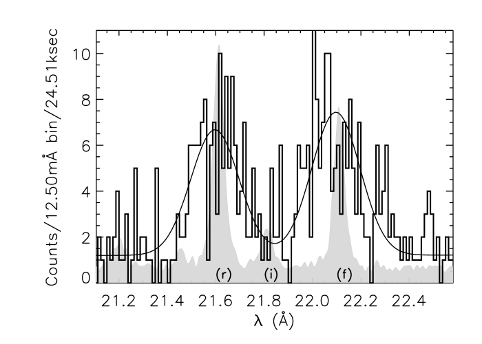
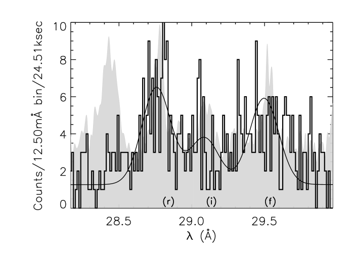
Figure 6: O vii (left) and N vi (right) He-like triplets with best-fitting one-component line templates. For O vii no intercombination line (expected at 21.8 Å) can be seen, while for the N vi triplet this line (expected at 29.1 Å) might be present. The intercombination lines are expected to show up with increasing electron densities. The smooth filled curve is that of Capella.

Apart from the lines of the He and H-like ions, it is difficult to make definite identifications of the other lines. Most lines that occur in the region from 30-50 Å are from transitions between excited states in Si, S, and Fe. It is difficult to check the plausibility of possible identifications since the $\Delta$n=0 resonance lines of the ions concerned lie at longer wavelengths than can be observed with Chandra. We have used the mean apparent wavelength shift and the mean line width of the identified lines to predict the rest-frame wavelengths and values of line widths of possible lines. Although the spectrum is noisy and some features are narrower than expected, it is possible that some lines of Si xii and S xiv are present. These are the S xiv 3p-2s transitions at 30.43 and 30.47 Å and the Si xii 3s-2p transitions at 45.52 and 45.69 Å. The Si xii 3p-2s transitions lie at $\sim 41$ Å and would not be observable as they occur within a region of instrumental insensitivity.
For the lines listed in Table 2 we calculate the sum of the line fluxes (corrected for N_H) and find a total line luminosity of $\sim 4\times 10^{27}$ erg s^-1.

4.5 Densities

From analyses of UV spectra Shore et al. (2003) reported values of hydrogen densities, n_H, between $1.25\times 10^{7}$ and $1.26\times 10^{8}$ cm^-3. In the X-ray regime no lines exist that can be used to measure n_e ($\approx$ n_H) below $10^{9}$ cm^-3. Since the X-ray lines are unlikely to be found in the same region as the UV lines we checked the density-sensitive line ratios in He i-like ions (e.g., Gabriel & Jordan, 1969; Ness et al., 2004). Unfortunately the signal to noise in the intersystem lines in N vi, O vii and Ne ix is too low to make quantitative analyses (see Figs. 3 and 6). Qualitatively, the upper limits to the intersystem lines suggest that n${}_{e}<2\times 10^{9}$ cm^-3.

4.6 Search for iron lines

From the bottom two panels of Fig. 3 it can be seen that in addition to the Ne lines identified in the spectrum of V382 Vel, some lines appear in the Capella spectrum that have no obvious counterparts in V382 Vel. These lines originate from Fe xvii to Fe xxi (see Ness et al., 2003), and the absence of these lines in V382 Vel indicates an enhanced Ne/Fe abundance ratio. Since V382 Vel is an ONeMg nova, a significantly enhanced Ne/Fe abundance (as compared to Capella) is expected. We have systematically searched for line emission from the strongest Fe lines in different ionization stages. We studied the emissivities of all iron lines below 55 Å predicted by the APEC database for different stages of ionization as a function of temperature. The strongest measureable line is expected to be that of Fe xvii at 15.01 Å. The spectral region around this line is shown in the upper left panel of Fig. 7, and there is no evidence for the presence of this line. The shaded spectrum is the arbitrarily scaled (as in Fig. 3) LETG spectrum of Capella, showing where emission lines from Fe xvii are expected. There is some indication of line emission near 15.15 Å, which could be O viii Ly_γ at 15.176 Å (Table 2), since the O viii Ly_β line at 16 Å is quite strong. The spectral region shown in Fig. 7 also contains the strongest Fe xviii line at 14.20 Å. Again, in the Capella spectrum there is clear Fe xviii emission, while in V382 Vel there is no indication of this line (a possible feature at 14.0 Å has no counterpart in the APEC database). Neither are the hotter Fe xxiii and Fe xxiv lines detected in this spectrum. We conclude that emission from Fe lines is not present in the spectrum.

4.7 Temperature structure and abundances

The lines observed are formed under a range of temperature conditions. We assume that collisional ionization dominates over photoionization and that the lines are formed by collisional excitations and hence find the emission measure distribution that can reproduce all the line fluxes. In Fig. 8 we show emission measure loci for 13 lines found from the emissivity curves $G_{i}(T)$ (for each line $i$ at temperature $T$) extracted from the Chianti database, using the ionization balance by Arnaud & Rothenflug (1985). The volume emission measure loci are obtained using the measured line fluxes $f_{i}$ (Table 2) and $EM_{i}(T)=4\pi\,{\rm d}^{2}(hc/\lambda_{i})(f_{i}/G_{i}(T))$ having corrected the fluxes for N_H. The emissivities $G_{i}(T)$ are initially calculated assuming solar photospheric abundances (Asplund et al., 2005). The solid smooth curve is the best-fitting emission measure distribution $EM(T)$, which can be used to predict all line fluxes $F_{i}=hc/\lambda_{i}\int G_{i}(T)\,EM(T)dT(4\pi{\rm d}^{2})^{-1}$. In each iteration step the line fluxes for the measured lines can be predicted ($F_{i}$) and, depending on the degree of agreement with the measured fluxes, the curve parameters can be modified (we used Powells minimization – see Press et al., 1992). In order to exclude abundance effects at this stage we optimized the reproduction of the temperature-sensitive line ratios of the Ly_α and He-like r lines of the same elements and calculated the ratios $R_{j}=f_{{\rm Ly},j}/f_{{\rm r},j}$, for Mg, Ne, O, and N and then compared these with the respective measured line ratios $r_{j}$ (see Schmitt & Ness, 2004). This approach constrains the shape of the curve, but not the normalization, which is obtained by additionally optimizing the O viii and O vii absolute line fluxes; the emission measure distribution is thus normalized to the solar O abundance. The goodness parameter is thus defined as

$$\chi^{2} = \sum_{j}\frac{(R_{j}-r_{j})^{2}}{\Delta r_{j}^{2}}$$

$$+\,(f_{\mbox{O\,{\sc vii}}}-F_{\mbox{O\,{\sc vii}}})^{2}/\Delta f_{\mbox{O\,{\sc vii}}}^{2}$$

$$+\,(f_{\mbox{O\,{\sc viii}}}-F_{\mbox{O\,{\sc viii}}})^{2}/\Delta f_{\mbox{O\,{\sc viii}}}^{2}$$

with $\Delta r$ and $\Delta f$ being the measurement errors of the indexed line ratios and fluxes. The emission measure distribution (solid red curve) is represented by a spline interpolation between the interpolation points marked by blue bullets. In the lower left we show the measured ratios (with error bars), and the best-fitting ratios (red bullets) showing that the fit has a high quality. We tested different starting conditions (chosen by using different initial interpolation points) and the fit found is stable.

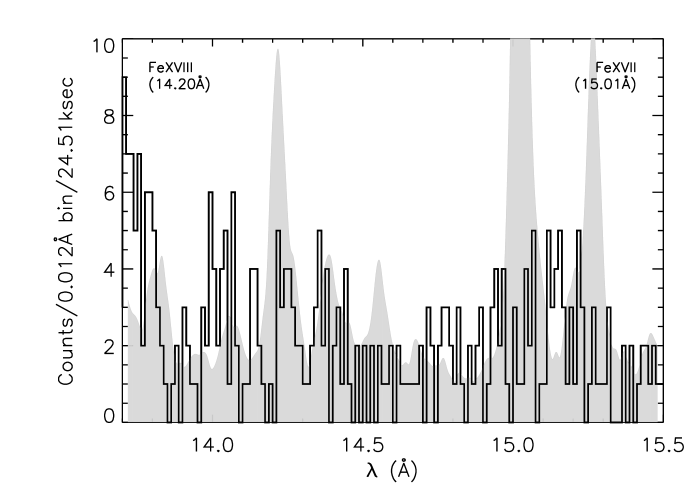
Figure 7: Spectral regions containing Fe xvii expected at 15.01 Å, and Fe xviii at 14.2 Å. No evidence for the presence of these lines can be seen. For comparison the Capella LETG spectrum is shown as smoothed filled curve.

We used the best-fitting emission measure distribution to predict the fluxes of the strongest lines in the spectrum and list the ratios of the measured and predicted fluxes in Table 3. It can be seen that for a given element the same trend is found for different ionization stages. If the mean emission measure distribution predicts less flux than observed, then the element abundance must be increased, to lower the loci to fit those of O.

Increased abundances (relative to O) are required for N and Ne (by a factor of 4), for Mg (by a factor of 2) and C and Si (by a factor of 1.4). The increase for C, based only on the 33.8-Å line is an upper limit, because the flux in this noisy line may be overestimated. The Mg and Si line fluxes have quite large uncertainties and the fitting procedure above $6\times 10^{6}$ K is less secure. The resulting values of N(N)/N(O) and N(Ne)/N(O) are 0.53 and 0.59, respectively, which are slightly lower than those of Shore et al. (2003), who found 0.63 and 0.79, respectively. The values of N(Mg)/N(O) and N(Si)/N(O) are 0.19 and 0.1, respectively, which are substantially larger than the values of 0.04 and 0.01 found by Shore et al. (2003). To avoid too much flux in the iron lines the value of N(Fe)/N(O) used must be reduced by $\sim 0.2-0.6$. This gives N(Fe)/N(O)$<0.04$.

The corrected emission measure loci are shown in the right-hand panel of Fig. 8, where it can be seen that the loci now form a smooth envelope reflecting a meaningful physical distribution. The $\chi^{2}$ value in the upper right corners of Fig. 8 represent the goodness with which the ratios and the O line fluxes are represented and how well all line fluxes (except iron) are represented. We have tested the effects of changing the values of N_H by a factor of two. This primarily affects the longer wavelength lines of C and N, leading to abundances (relative to O) that increase with increasing values of the assumed N_H. In Table 3 we give examples of the results for C and N using values of N_H that are twice the original value of $1.2\times 10^{21}$ cm^-2 and half of this value. The absolute emission measure values increase by about 30 per cent when N_H is a factor of two higher and decrease by about 20 per cent when N_H is lowered by a of factor two. Without a measurement of the density we cannot derive a model from the absolute emission measures. The values of the emission measures are consistent with those given by Orio (2004).
We stress that only the average properties of the expanding shell can be derived. Since we have evidence that the lines are produced non-uniformly, there may be different abundances in different regions of the shell.

Table 3: Ratios of measured and predicted line fluxes from the best-fit emission measure curve in the left panel of Fig. 8. These give the corrections required to the adopted solar element abundances^[a] (Asplund et al., 2005), relative to O.

ion	R[b]	ion	R[b]	ion	R[b]
C vi	$<$1.3	Si xiii	1.37	Mg xii	2.97
N vii	3.92	N vi	3.92	Mg xi	1.88
O viii	0.98	O vii	0.91	Fe xvii	$<$0.15
Ne x	3.79	Ne ix	3.97	Fe xviii	$<$0.60
with half the value of NH
C vi	0.82	N vi	3.65	N vii	3.66
with double the value of NH
C vi	3.38	N vi	4.48	N vii	4.49

^[a] Adopted solar abundances (relative to O) C/O: 0.537, N/O: 0.132, Ne/O: 0.151, Mg/O: 0.074, Si/O: 0.071, Fe/O: 0.062.

^[b] Ratio of measured to predicted line fluxes.

5 Discussion

The previous X-ray observations of Nova V382 Vel were carried out at a lower spectral resolution making detection of line features difficult. Both BeppoSAX and Chandra (ACIS-I) found that the nova was extremely bright in the Super Soft Phase (Orio et al., 2002; Burwitz et al., 2002). Orio et al. tried to fit their observations with Non-LTE atmospheres characteristic of a hot WD with a ‘forest’ of unresolved absorption lines, but no reasonable fit was obtained. These authors determined that even one or two unresolved emission lines superimposed on the WD atmosphere could explain the spectrum, and suggested that the observed ‘supersoft X-ray source’ was characterized by unresolved narrow emission lines superimposed on the atmospheric continuum’ (Orio et al., 2002). The LETG spectrum obtained on 14 February 2000 shows emission lines with only a weak continuum. We conclude that nuclear burning switched off before 2000 February and the emission peak at $\sim 0.5$ keV reflects continuum emission from nuclear burning.
The ‘afterglow’ shows broad emission lines in the LETG spectrum reflecting the velocity, temperature and abundance structure of the still expanding shell. The X-ray data allow an independent determination of the absorbing column-density from the ratio of the observed H-like Ly_α and Ly_β line fluxes, leading to a value consistent with determinations in the UV. The value measured from the LETG spectrum appears to represent the constant interstellar absorption value. Some of the lines consist of several (at least two) components moving with different velocities. These structured profiles are different for different elements. While the O lines show quite compact profiles, the Ne lines show a double feature indicative of two components.
No Fe lines could be detected although lines of Fe xvii and Fe xviii are formed over the temperature range in which the other detected lines are formed. We attribute this absence of iron lines to an under-abundance of Fe with respect to that of O. Since we are observing nuclearly processed material from the white dwarf, it is more likely that elements such as N, O, Ne, Mg and possibly C and Si are over-abundant, rather than Fe being under-abundant. Unfortunately, no definitive statements about the density of the X-ray emitting plasma can be made. Thus neither the emitting volumes nor the radiative cooling time of the plasma can be found.

6 Conclusions

We have analyzed the first high-dispersion spectrum of a classical nova in outburst, but it was obtained after nuclear burning had ceased in the surface layers of the WD. Our spectrum showed strong emission lines from the ejected gas allowing us to determine velocities, temperatures, and densities in this material. We also detect weak continuum emission which we interpret as emission from the surface of the WD, consistent with a black-body temperature not exceeding $\sim 3\times 10^{5}$ K. Our spectrum was taken only 6 weeks after an ACIS-S spectrum that showed the nova was still in the Super Soft X-ray phase of its outburst. These two observations show that the nova not only turned off in 6 weeks but declined in radiated flux by a factor of 200 over this time interval. This, therefore, is the third nova for which a turn-off time has been determined and it is, by far, the shortest such time. For example, ROSAT observations of GQ Mus showed that it was declining for at least two years if not longer (Shanley et al., 1995) and ROSAT observations of V1974 Cyg showed that the decline took about 6 months (Krautter et al., 1996). Since the WD mass is not the only parameter, but a fundamental one determining the turn-off time of the supersoft X-rays, the mass of V382 Vel may be larger than the two other novae (see also Krautter et al., 1996).

The emission lines in our spectrum have broad profiles with FWHM indicating ejection velocities exceeding 2900 km s^-1. However, lines from different ions exhibit different profiles. For example, O viii, 18.9 Å, and N vii, 24.8 Å, can be fit by a single Gaussian profile but Ne ix, 13.45 Å, and Ne x, 12.1 Å, can only be fit with two Gaussians. We are then able to use the emission measure distribution to derive relative element abundances and find that Ne and N are significantly enriched with respect to O. This result confirms that the X-ray regime is also able to detect an ONeMg nova and strengthens the necessity of further X-ray observations of novae at high dispersion.

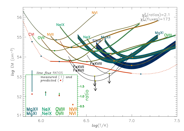
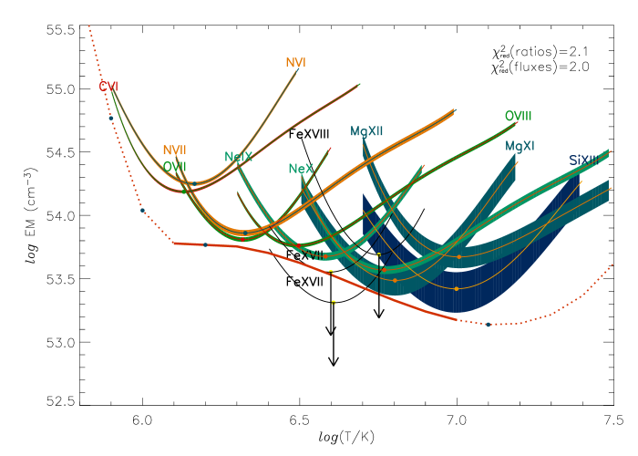
Figure 8: Left: Emission measure loci of the strongest lines using solar photospheric abundances. The solid red curve marks the best fit reproducing the line ratios of Ly_α vs. He-like r line of Mg, Ne, O and N as well as the measured line fluxes of O viii and O vii. The discrepancies in the loci of the other lines are attributed to abundance effects. The loci for iron are upper limits. The inset illustrates how well the indicated line ratios are reproduced. Right: The emission measure loci corrected by factors (Table 3) to give the corrections to the abundances of the respective elements relative to O. The solid curve is the best fit reproducing the line fluxes. Note that the y-axis has a different scale than in the left panel. The legends give the $\chi^{2}$ values for the reproduction of the line ratios and of the line fluxes.

References

- Anders & Grevesse (1989) Anders E., Grevesse N., 1989, Geochimica et Cosmochimica Acta, 53, 197
- Argiroffi et al. (2003) Argiroffi C., Maggio A., Peres G., 2003, A&A, 404, 1033
- Arnaud & Rothenflug (1985) Arnaud M., Rothenflug R., 1985, A&AS, 60, 425
- Asplund et al. (2005) Asplund M., Grevesse N., Sauval A. J., 2005, ASP Conf. Series. In press (astro-ph/0410214 v2 10 Oct 2004)
- Balucinska-Church & McCammon (1992) Balucinska-Church M., McCammon D., 1992, ApJ, 400, 699
- Burwitz et al. (2002) Burwitz V., Starrfield S., Krautter J., Ness J.-U., 2002, in Hernanz M., José J., eds., AIP Conf. Proc. Vol. 637: Classical Nova Explosions. American Institute of Physics, p. 377
- Cash (1979) Cash W., 1979, ApJ, 228, 939
- Della Valle et al. (2002) Della Valle M., Pasquini L., Daou D., Williams R. E., 2002, A&A, 390, 155
- Drake et al. (2003) Drake J. J., Wagner R. M., Starrfield S., Butt Y., Krautter J., Bond H. E., Della Valle M., Gehrz R. D. et al. 2003, ApJ, 584, 448
- Gabriel & Jordan (1969) Gabriel A. H., Jordan C., 1969, MNRAS, 145, 241
- Gilmore (1999) Gilmore A. C., 1999, in Green D. W. E., ed., IAU Circular Vol. 7179, 1
- Kashyap & Drake (2000) Kashyap V., Drake J. J., 2000, Bulletin of the Astronomical Society of India, 28, 475
- Krautter (2002) Krautter J., 2002, in Hernanz M., José J., eds., AIP Conf. Proc. Vol. 637: Classical Nova Explosions. American Institute of Physics, p. 345
- Krautter et al. (1996) Krautter J., Oegelman H., Starrfield S., Wichmann R., Pfeffermann E., 1996, ApJ, 456, 788
- Mazzotta et al. (1998) Mazzotta P., Mazzitelli G., Colafrancesco S., Vittorio N., 1998, A&AS, 133, 403
- Mukai & Ishida (2001) Mukai K., Ishida M., 2001, ApJ, 551, 1024
- Mukai & Swank (1999) Mukai K., Swank J., 1999, in Green D. W. E., ed., IAU Circular Vol. 7206, 3
- Ness & Wichmann (2002) Ness J.-U., Wichmann R., 2002, Astronomische Nachrichten, 323, 129
- Ness et al. (2003) Ness J.-U., Brickhouse N. S., Drake J. J., Huenemoerder D. P., 2003, ApJ, 598, 1277
- Ness et al. (2004) Ness J.-U., Güdel M., Schmitt J. H. M. M., Audard M., Telleschi A., 2004, A&A, 427, 667
- Ness et al. (2001) Ness J.-U., Mewe R., Schmitt J. H. M. M., Raassen A. J. J., Porquet D., Kaastra J. S., van der Meer R. L. J., Burwitz V., Predehl P., 2001, A&A, 367, 282
- Ness et al. (2003) Ness J.-U., Starrfield S., Burwitz V., Wichmann R., Hauschildt P., Drake J. J., Wagner R. M., Bond H. E. et al. 2003, ApJL, 594, L127
- Orio (2004) Orio M., 2004, in Tovmassian G. & Sion E., eds., Revista Mexicana de Astronomia y Astrofisica Conference Series Vol. 20. Instituto de Astronomía, Universidad Nacional Autónoma de México, p. 182
- Orio et al. (2002) Orio M., Parmar A. N., Greiner J., Ögelman H., Starrfield S., Trussoni E., 2002, MNRAS, 333, L11
- Orio et al. (2001) Orio M., Parmar A., Benjamin R., Amati L., Frontera F., Greiner J., Ögelman H., Mineo T., Starrfield S., Trussoni E., 2001, MNRAS, 326, L13
- Press et al. (1992) Press W. H., Teukolsky S. A., Vetterling W. T., Flannery B. P., 1992, Numerical recipes in FORTRAN. The art of scientific computing. Cambridge University Press, 1992, 2nd ed.
- Schmitt & Ness (2004) Schmitt J. H. M. M., Ness J.-U., 2004, A&A, 415, 1099
- Shanley et al. (1995) Shanley L., Ogelman H., Gallagher J. S., Orio M., Krautter J., 1995, ApJL, 438, L95
- Shore et al. (2003) Shore S. N., Schwarz G., Bond H. E., Downes R. A., Starrfield S., Evans A., Gehrz R. D., Hauschildt P. H. et al. 2003, AJ, 125, 1507
- Starrfield (1989) Starrfield S., 1989, in M. Bode, A. Evans eds., Classical Novae. Wiley, New York, p. 39
- Starrfield et al. (1991) Starrfield S., Truran J. W., Sparks W. M., Krautter J., 1991, in Malina R. F., Bowyer S., eds., Extreme Ultraviolet Astronomy. Pergamon Press, New York, p. 168
- Woodward et al. (1999) Woodward C. E., Wooden D. H., Pina R. K., Fisher R. S., 1999, in Green D. W. E., ed., IAU Circular Vol. 7220, 3