Absolute polarisation position angle profiles of southern pulsars at 1.4 and 3.1 GHz

Abstract

We present here a direct comparison of the polarisation position angle (PA) profiles of 17 pulsars, observed at 1.4 and 3.1 GHz. Absolute PAs are obtained at each frequency, permitting a measurement of the difference in the profiles. By doing this, we obtain more precise rotation measure (RM) values for some of the pulsars in the current catalogue. We find that, apart from RM corrections, there are small, pulse longitude dependent differences in PA with frequency. Such differences go beyond the interpretation of a geometrical origin. We describe in detail the PA evolution between the two frequencies and discuss possible causes, such as orthogonal and non-orthogonal polarisation modes of emission. We also use the PA and total power profiles to estimate the difference in emission height at which the two frequencies originate. In our data sample, there are changes in the relative strengths of different pulse components, especially overlapping linearly polarised components, which coincide with intrinsic changes of the PA profile, resulting in interesting PA differences between the two frequencies.

1 Introduction

Shortly after the original discovery of pulsars, Radhakrishnan & Cooke (1969) developed a model of emission which has subsequently been used to interpret pulsar polarisation. According to this model, pulsar radiation is polarised along, or orthogonal to, the open magnetic field lines of the strong dipolar magnetic field that surrounds the star. As the beam of the pulsar sweeps past the line of sight of the observer, the position angle (PA) of the linear polarisation rotates, resulting in the well known S-shaped curves of PA versus pulse phase seen in many pulsars. The angles which determine the sweep of the PA are the inclination angle $\alpha$ between the magnetic and rotational axes and the impact parameter $\beta$, which is the smallest angle between the locus of the line of sight on the pulsar beam and the magnetic axis. This rotating vector model (RVM) has been used in some cases to infer the geometrical angles of pulsars from polarisation observations.

Despite the initial success of the RVM, numerous attempts to fit polarimetric data demonstrated that in many cases, the parameters of the fit were poorly constrained, mainly due to the restricted longitude over which pulsars emit. For instance, in the case of Blaskiewicz et al. (1991), who are primarily concerned with the point of steepest gradient of the PA swing, the fitted parameters $\alpha$ and $\beta$ at 430 and 1418 MHz rarely agree. The authors attribute this to very large error estimates, often as large as hundreds of degrees. The same is seen in another set of published RVM fits at multiple radio frequencies (von Hoensbroech & Xilouris, 1997a). Mitra & Li (2004) recently presented RVM fits for 6 pulsars, to data obtained at multiple frequencies (4 to 6 frequencies for each pulsar). Similarly to Blaskiewicz et al. (1991), the fitted parameters (especially $\alpha$) generally do not agree between the different frequencies, despite the claim of the authors to the contrary. In a remarkably complete treatment, Everett & Weisberg (2001) summarise the problem and demonstrate the difficulties in obtaining a unique RVM solution. They attempt RVM fits on their data, obtaining reliable results for only 10 out of the 70 pulsars in their sample. Even in the limited cases, the fitted parameters are not always in agreement with previously published results.

Early observations also showed that average pulse profiles become narrower with increasing frequency. The model of Ruderman & Sutherland (1975) suggests that the frequency of emission is related to the local plasma density, which drops off at higher altitudes from the surface of the star. This leads to a natural radius-to-frequency mapping (RFM), with higher frequencies originating closer to the pulsar surface. In the dipolar magnetic field structure, the open field lines spread out at greater altitudes, explaining the broader widths of profiles at lower frequencies (Cordes, 1978). Although the exact height at which a particular frequency is emitted depends on the nature of the emission mechanism (Melrose, 2000), some sort of RFM appears to underly the observations.

To first order, the PA at a given pulse longitude is fixed, irrespective of the emission height. The consequences of RFM on the PA lie mainly in second order effects, such as relativistic effects within the pulsar light cylinder. Blaskiewicz et al. (1991) showed that due to such effects, the centroid of the PA swing is delayed with respect to the centroid of the total intensity by an amount proportional to the radius at which the radiation originates, providing a method to estimate relative emission heights in the magnetosphere. Such calculations agreed well with the heights inferred by the changing widths of average profiles.

In a comparison of data from PSR B0329+54 at two frequencies,Malov & Suleimanova (1998) showed that the position of the pair of outer components changes relative to the central component, due to effects of retardation and aberration. A method for estimating emission altitudes was subsequently proposed by Gangadhara & Gupta (2001), who exploit the fact that components originating close to the magnetic axis are emitted from much lower altitudes than pairs of components that flank them. In pulsar profiles with an appropriate configuration, the relativistic phase shift between the central (core) component and the middle of the outer component pair provides the only information necessary to compute emission heights, as demonstrated in a refinement of the method of Gangadhara & Gupta (2001) by Dyks et al. (2004). The emission altitudes using this relativistic method are generally larger than those of the Blaskiewicz et al. (1991) method. In practice, the main difficulty of estimating emission heights in this way relates to the limited pulsar profiles with a central component and outer components that can be unambiguously identified as a pair.

There are several reasons that cause observed PAs to diverge from the RVM. The first and probably best documented phenomenon is orthogonally polarised modes (OPM) in pulsar emission (e.g. Manchester et al., 1975; Backer et al., 1975; Cordes et al., 1978). These result in parts of the PA profile being $90\degr$ offset to the main swing, an effect which can be identified and accounted for. Also, OPMs are frequency dependent (e.g. Stinebring et al., 1984; Karastergiou et al., 2002), which results in different PA profiles at different frequencies, the higher frequencies showing more occurrences of $90\degr$ discontinuities.

An additional source of the PA dependence on frequency may originate from non-orthogonal polarisation modes, identified first by Backer & Rankin (1980). Ramachandran et al. (2004) recently showed that the different spectral behaviour of quasi-orthogonal modes in PSR B2016+28 results in a change in the PA swing over a very narrow frequency range. Karastergiou et al. (2005) claim that the spectral behaviour of the total power and linear polarisation in different components can also be attributed to different spectra of the orthogonal modes. The possibility of variable PA profiles at different frequencies then naturally arises.

Michel (1991) considered Faraday rotation in the magnetospheres of pulsars as the cause of complexity in the PA profiles of pulsars. However, he argued that the physical grounds for this process are lacking and subsequently no attempt was made to observationally identify this phenomenon.

All of the above mechanisms that distort the simple geometric nature of the RVM, also have some form of inherent dependence on frequency. We therefore proceeded to investigate this by presenting for the first time direct comparisons of the PA swings of 17 pulsars between 1.375 and 3.1 GHz. In doing so, we document the nature of the frequency evolution of the PA, which we discuss in the context of the above physical processes and models. The purpose of our analysis is to specifically avoid RVM fits to our data and geometrical interpretations which rely upon these fits. On the contrary, instead of comparing the PA profiles to a badly constrained curve, we compare them as precisely as possible to each other in an unbiased approach to study PA changes. We believe this approach is warranted given the nature of most PA profiles in our data and the difficulties in fitting RVM curves over very small longitude ranges.

In Section 2 we describe the observations. In Section 3 we present a method by which we align the profiles at the two different frequencies using the absolute PA values, which also permit us to determine very precise RMs. In Section 4 we discuss the polarisation profiles and compare them to previous profiles at other frequencies. In the final parts of this paper, we discuss the differences between the profiles at the two frequencies and possible interpretations in the context of the above models for the origin and frequency evolution of PA profiles.

2 The observations

The observations were carried out using the Parkes radio telescope on 2004 August 31 and September 1. We used the H-OH receiver at a central frequency of 1.375 GHz with a bandwidth of 256 MHz and the 10/50 cm receiver at a central frequency of 3.1 GHz with a bandwidth of 512 MHz. In both cases, the backend correlator subdivided the total bandwidth into 1024 frequency channels and also recorded 1024 longitude bins per pulse period. The receivers have orthogonal linear feeds and also have a pulsed cal signal which is injected at a position angle of 45° to the two feed probes.

The pulsars were observed for 30 minutes at each frequency. Prior to the pulsar observation a 3 min observation of the pulsed cal was made. The data were written to disk in FITS format for subsequent off-line analysis. Data analysis was carried out using the PSRCHIVE software package (Hotan et al., 2004).

Name		Period	W$10$		RM		RM reference
J2000	B1950	ms	$\nu_{1}$	$\nu_{2}$	rad/m2
			deg	deg	New	Previous
J0738$-$4042	B0736-40	375	32	30	14$\pm 0.5$	14	Taylor et al. (1993)
J0742$-$2822	B0740-28	167	16	16	150$\pm 0.5$	156	Han et al. (1999)
J0835$-$4510	B0833-45	89	14	16	32$\pm 0.5$	38	Hamilton et al. (1977)
J0837$-$4135	B0835-41	752	5	6	146$\pm 1.0$	136	Taylor et al. (1993)
J0942$-$5552	B0940-55	664	26	29	$-$62$\pm 0.8$	$-$62	Taylor et al. (1993)
J1056$-$6258	B1054-62	422	32	32	$-$1 or 6$\pm 0.5$	4	Costa et al. (1991)
J1157$-$6224	B1154-62	401	45	48	507$\pm 2.5$	508	Taylor et al. (1993)
J1243$-$6423	B1240-64	388	7	8	162$\pm 1.0$	158	Taylor et al. (1993)
J1326$-$5859	B1323-58	478	17	16	$-$586$\pm 0.7$	$-$580	Costa et al. (1991)
J1327$-$6222	B1323-62	530	11	11	$-$319$\pm 0.8$
J1356$-$6230	B1353-62	456	32	27	$-$580$\pm 1.7$
J1359$-$6038	B1356-60	127	14	14	39 or 37$\pm 0.5$	33	Han et al. (1999)
J1602$-$5100	B1558-50	864	11	13	79$\pm 1.3$	72	Taylor et al. (1993)
J1644$-$4559	B1641-45	455	14	11	$-$618$\pm 0.5$	$-$611	Taylor et al. (1993)
J1752$-$2806	B1749-28	562	8	8	91$\pm 3.0$	96	Hamilton & Lyne (1987)
J1807$-$0847	B1804-08	164	28	28	171$\pm 1.8$	166	Hamilton & Lyne (1987)
J1825$-$0935	B1822-09	769	22	21	68$\pm 0.7$	65	Hamilton & Lyne (1987)

Table 1: The list of pulsars and their parameters. $\nu_{1}$ and $\nu_{2}$ correspond to 1.375 and 3.1 GHz respectively.

We used standard techniques to calibrate the relative gains and phases of the two linear feed probes. The pulsed cal is injected at 45° to both probes so that its intrinsic signal can be assumed to be 100 per cent polarised in Stokes $U$. Gain corrections can be made by comparing the observed Stokes $Q$ with Stokes $I$ and phase corrections can be made by comparing the observed Stokes $U$ with Stokes $V$ on a channel by channel basis in the output data. Following this calibration $Q$ and $U$ can be further rotated to correct for the angle which the feed probes make to true north and for the parallactic angle of the source at the time of the observation. At the end of this procedure we have the intrinsic PA of the radiation just above the feed at a particular frequency. PA values are only computed when the linear polarisation exceeds the noise by a factor of 5.

To obtain the PA at the pulsar, the Faraday rotation both through the Earth’s ionosphere and the interstellar medium must be corrected for. This is done in a two stage process. First, we fit for the RM across the 256 MHz band at 1369 MHz. This yields an RM with an error of order $\pm$5 rad m^-2. The PAs at both 1.375 and 3.1 GHz can be rotated by an amount given by

$$\theta=\frac{c^{2}\,\,\,{\rm RM}}{\nu^{2}}$$ (1)

where $c$ is the speed of light and $\nu$ the observing frequency. A more precise RM can then be produced by comparing the PAs at both frequencies, using a least squares fitting technique as described in more detail below.

3 Data analysis

A new approach is used in this paper to align profiles at 1.375 and 3.1 GHz. Initially, we slide one PA profile over the other in the horizontal, pulse-longitude direction, in steps of one bin of data. At every step of shift $dx$, we measure the average offset $d$PA between the two PA profiles

$$d{\rm PA}_{dx}=\frac{1}{N}\sum_{i=1}^{N}{\rm PA}1_{i}-{\rm PA}2_{i},$$ (2)

where $N$ is the overlapping number of data bins which have a PA measurement at both frequencies, $i$ the index of each such bin and PA1 and PA2 the value of the PA at that bin at 1.375 and 3.1 GHz respectively. Then, we calculate a normalised chi-square between the two sets of data, considering their average PA offset, according to the equation

$$\chi^{2}_{dx}=\frac{1}{N}\sum_{i=1}^{N}\frac{({\rm PA}1_{i}-{\rm PA}2_{i}-d{\rm PA}_{dx})^{2}}{2(\sigma_{{\rm PA}1,i}^{2}+\sigma_{{\rm PA}2,i}^{2})},$$ (3)

where $\sigma_{{\rm PA}1}$ and $\sigma_{{\rm PA}2}$ are the uncertainties in the PA measurements. As shown later, the instances of orthogonal PAs at the two frequencies are few and do not influence the value of $\chi^{2}_{dx}$. Despite this, if any instantaneous difference in the PA is greater than $45\degr$, we assign the PA difference the complementary value to $90\degr$, thus avoiding great dPA values in the case of orthogonal PAs at the two frequencies. We then shift the profile by one bin and repeat the process, thus yielding a table of $\chi^{2}$ as a function of the shift $dx$. The value of $dx$ that corresponds to $\chi^{2}_{min}$ is chosen as the shift in pulse-longitude to align the two profiles, and the corresponding average $d$PA is used to apply a vertical shift.

The vertical shift that is required to align the profiles can be achieved with a correction in the RM value and therefore by calculating the mean $d$PA offset we are computing a very accurate RM. The error on the RM then corresponds to the error in the mean $d$PA, which is

$$\sigma_{d\rm PA}=\frac{1}{N}\sum_{i=1}^{N}\sqrt{\sigma_{{\rm PA}1,i}^{2}+\sigma_{{\rm PA}2,i}^{2}}$$ (4)

The contributions to the measured values of RM arising in the ionosphere have been estimated by integrating a time-dependent model of the ionospheric electron density and geomagnetic field through the ionosphere along the sight line between the telescope and the pulsar. The average contribution is found to be $\sim-1$ rad m^-2.

4 Results

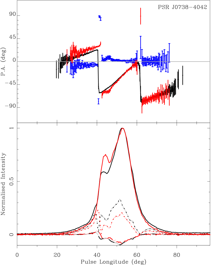
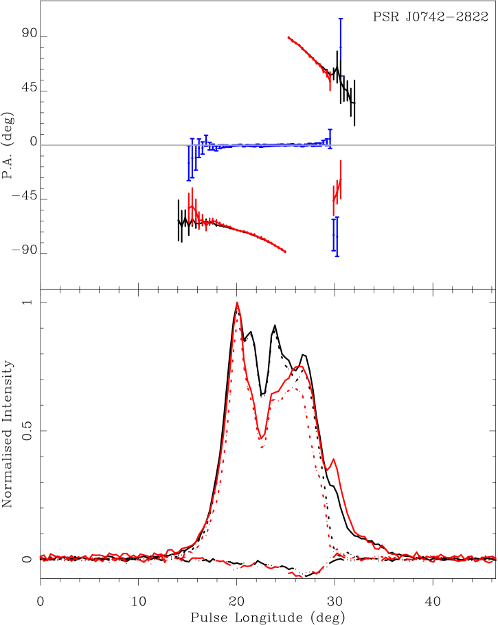
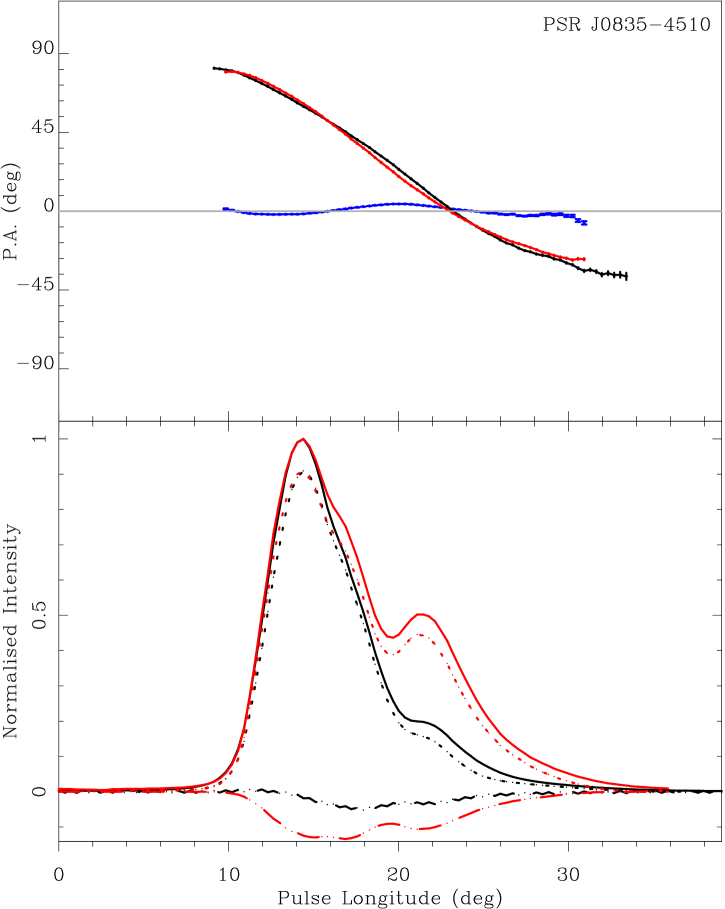
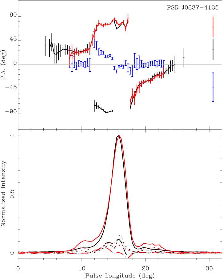
Figure 1: Overlaid polarisation profiles at 1.375 (black lines) and 3.1 GHz (red). In the lower panel of each figure, the solid lines denote total power, doted lines linear polarisation and dash-dotted lines circular polarisation. In the upper panel, the absolute PAs are shown for 1.375 and 3.1 GHz, following the same colour convention. Also, the error-bars with riser lines (blue) denote the difference between the two PAs, where there is a measurement at both frequencies.

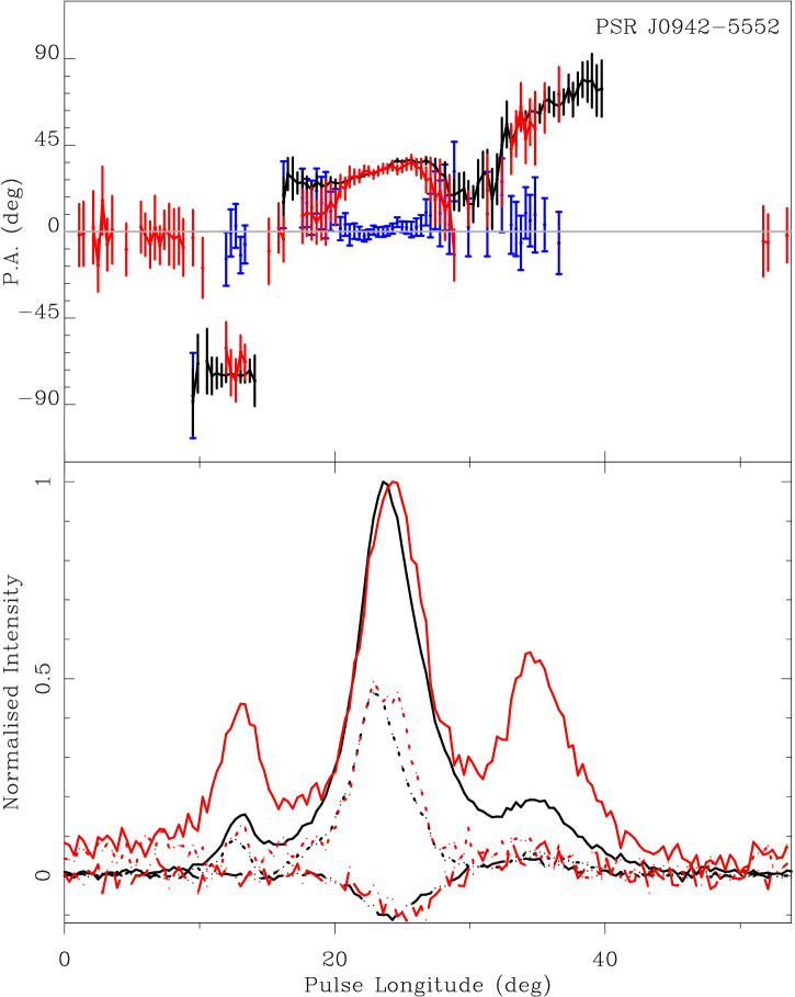
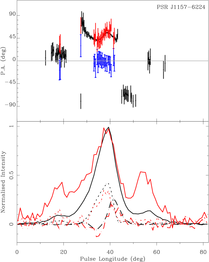
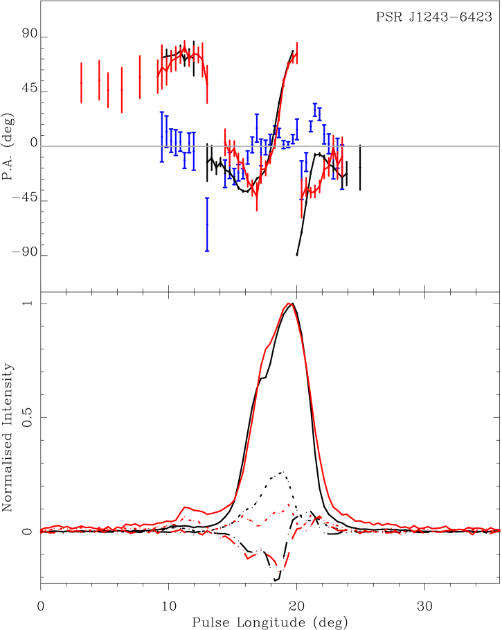
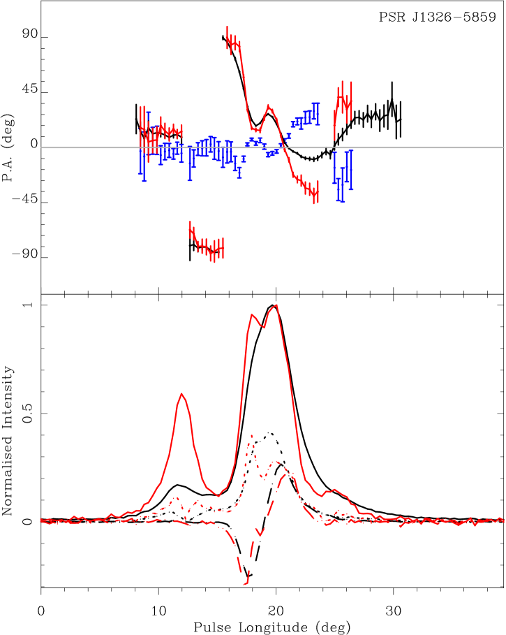
Figure 1: - continued.

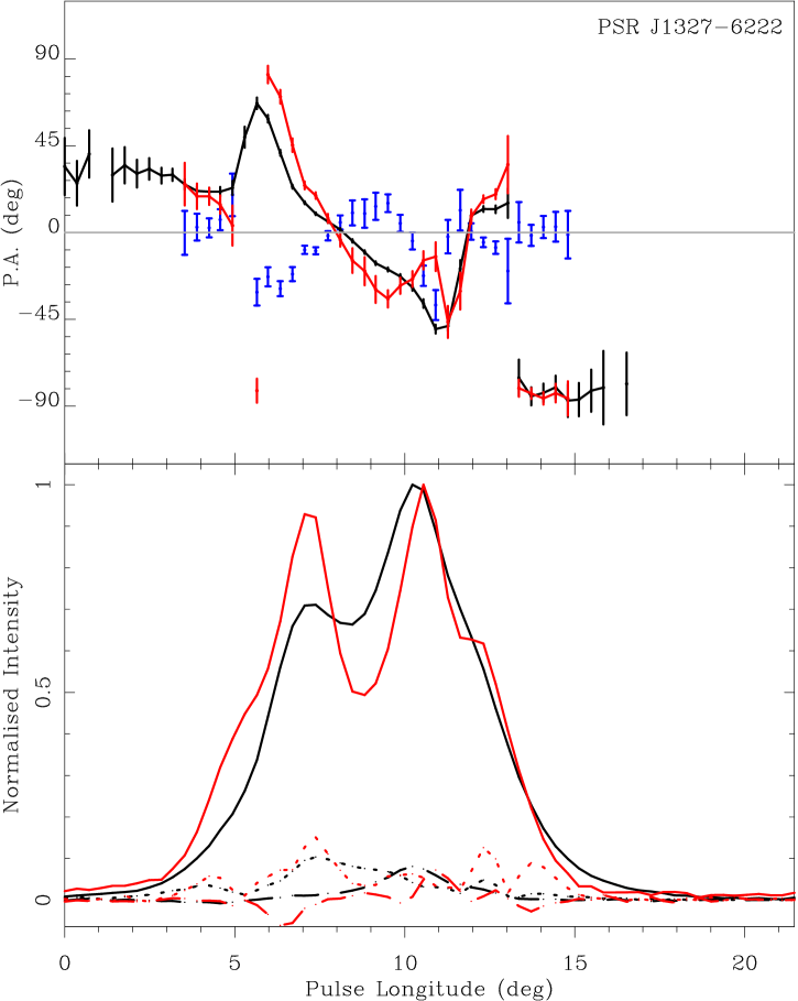
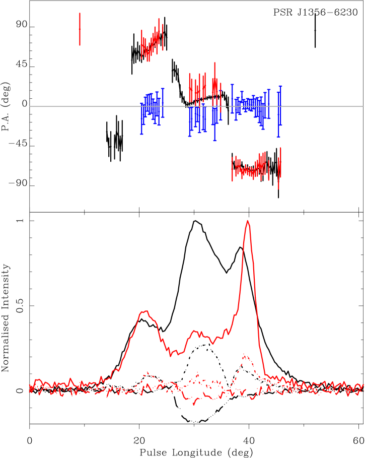
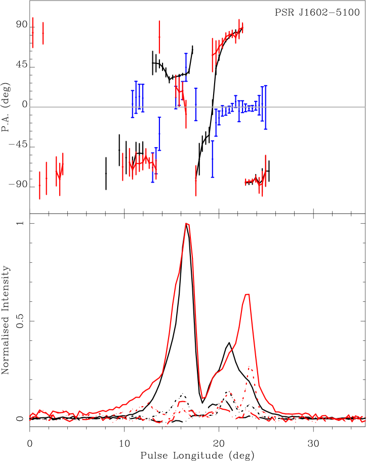
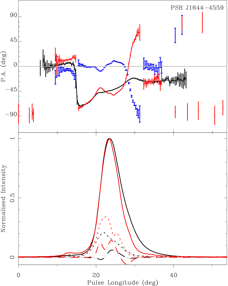
Figure 1: - continued.

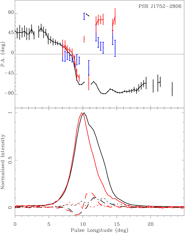
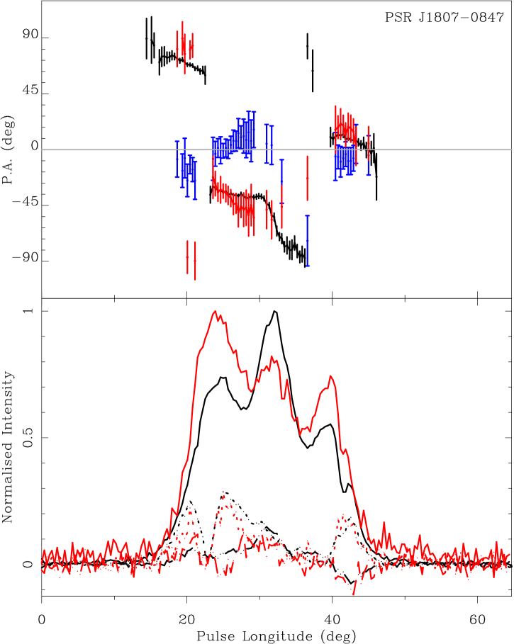
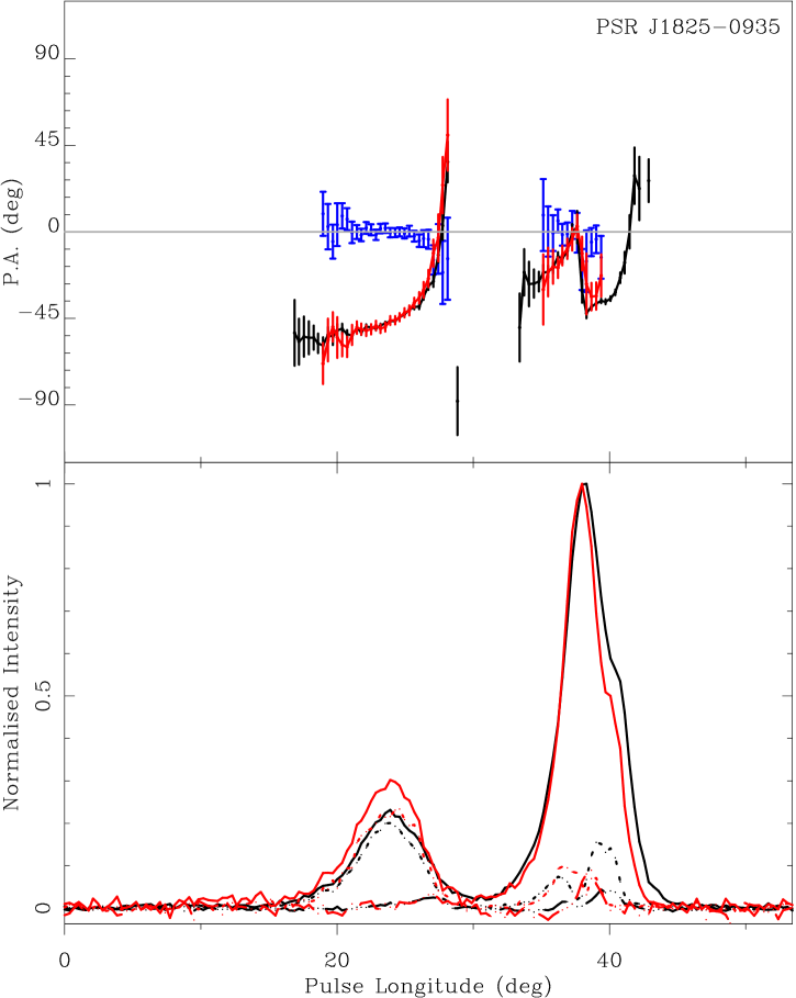
Figure 1: - continued.

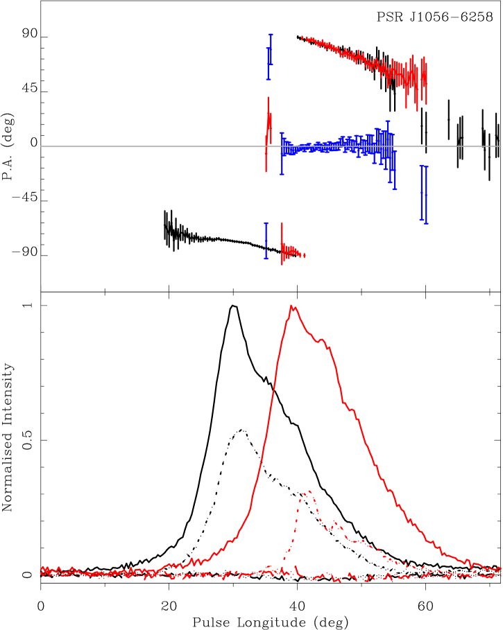
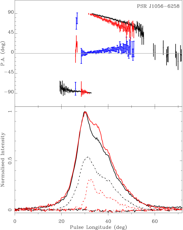
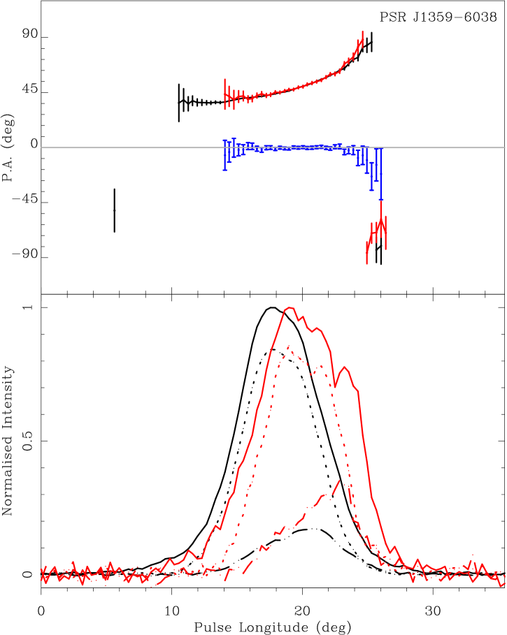
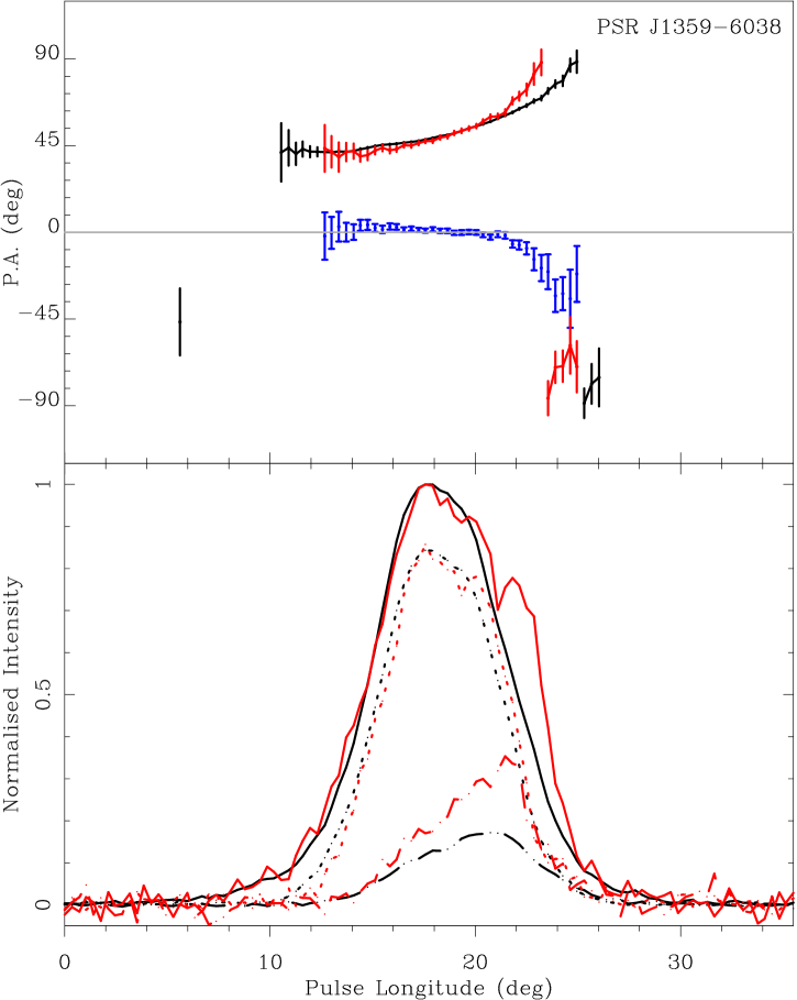
Figure 2: Same as Figure 1. The top two plots show PSR J1056$-$6258, the profile alignment performed on PA (left) and total power (right). The bottom two plots show the same for PSR J1359$-$6038. The offset between the two alignment methods is 10.7 ms for J1056$-$6258 and 0.7 ms for J1359$-$6038.

Table 1 shows the list of sources, their rotation period, the pulse widths at the 10% level of the peak flux density at both frequencies and the RM, after removing the ionospheric contribution. For comparison, we provide the current published RM values where available.

For an accurate comparison between the polarimetric profiles at 1.375 and 3.1 GHz, we have overlaid them for each pulsar, as shown in Figure 1. Due to the steep flux density spectrum of pulsars, the sources are much brighter at 1.375 than at 3.1 GHz. To further facilitate comparisons, we have normalised the flux density at both frequencies with respect to the peak of the profile. In doing so, the relative spectral dependence of the various components of the pulse becomes evident. In most of the pulsars presented here, the strongest profile component is the same at both frequencies. In these cases, the normalisation also permits direct comparisons between the fractional polarisation of these components. We also draw a comparison with previous data at 400 MHz (Hamilton et al., 1977), 600 MHz (McCulloch et al., 1978), 800 and 950 MHz (van Ommen et al., 1997) and 1612 MHz (Manchester et al., 1980) where appropriate.

J0738$-$4042 (B0736$-$40). The most striking feature of this pulsar is the smooth PA swing, which is broken twice by orthogonal jumps at the leading and trailing side of the profile at both 1.375 and 3.1 GHz. In fact there is little evolution of the polarisation profile between these frequencies, despite an increase of the total intensity of the leading component compared to the main peak of the profile at 3.1 GHz. The orthogonal jump in the leading component occurs exactly at the longitude where both linear and circular polarisation are zero and is accompanied by a change in the circular polarisation sense at both frequencies. This is also true for the trailing component jump, although the change in handedness of the circular polarisation is not as prominent. Drawing a comparison between our profiles and previous profiles at other frequencies, we focus on the leading component. The pulse longitude at which the first PA jump occurs shifts from the notch between the leading and middle component at 631 MHz to a slightly earlier longitude at 950 MHz. At that frequency, a second local minimum of linear polarisation appears at the pulse longitude of the notch. Surprisingly, the 1612 MHz profile shows the PA in the region between the local minima in linear polarisation following the previous swing and the jump occurring at the notch, similar to the 631 MHz data. In the 1.375 GHz profile shown here, the PA agrees with the 950 MHz data. The most plausible picture therefore, involves a change in dominant OPM between the two local minima of linear polarisation, occurring between 631 and 950 MHz and subsequently shifting the pulse longitude of the PA jump at frequencies above 950 MHz.

The comparison of PAs at 1.375 and 3.1 GHz shows that not all three segments of the PA profile align. Depending on the choice of RM, either the first or the second and third parts match. We have chosen the latter in Figure 1, and the differences in PA in the second and third segments are zero within the uncertainties. Note that the alignment method results in alignment in the total power of the main peak despite the misalignment of the linear polarisation.

J0742$-$2822 (B0740$-$28). The total power profiles at 1.375 and 3.1 GHz have the same overall structure. The leading part is made up of two overlapping components, the middle part of three and the trailing part of a narrow and a broad component (seven components are also suggested in Kramer 1994). However, the ratios of the component strengths are different at the two frequencies. In the above order, the first, fourth and fifth components have flatter spectra than the second and third components. Arguably, the same is true for the two trailing components with respect to components two and three. Both profiles are highly linearly polarised with a small amount, right-hand circular polarisation across the pulse, in agreement with earlier observations. The only obvious difference in the PA profiles is a $90\degr$ jump in the penultimate component at 3.1 GHz, not seen previously at other frequencies. The best alignment in PA also aligns the total power.

Gould & Lyne (1998) have observed this pulsar in full polarisation at frequencies up to 1642 MHz, while von Hoensbroech & Xilouris (1997b) have provided profiles at 4.85 GHz and 10.55 GHz. The 4.85 GHz profile does not demonstrate the orthogonal PA jump in the trailing component and the 10.55 GHz profile lacks a measurement of position angle in this component due to the low S/N of the linearly polarised flux. Careful investigation of the frequency dependence of the polarisation in the trailing component will be useful in determining whether there is a monotonic frequency behaviour of the strength of each OPM. If so, there should be a frequency above which the dominant mode switches (Karastergiou et al., 2005). Also, in the trailing component of the 3.1 GHz profile, the mean circular polarisation is very small across the component. Similar behaviour (i.e. a drop in the mean linear polarisation, orthogonal PAs and zero mean circular polarisation) has been observed in a number of pulsars which show wide distributions of circular polarisation, with many instances of high left- and high right-hand circular polarisation, resulting in a considerably higher value for the mean $|V|$ (Karastergiou et al., 2003; Karastergiou & Johnston, 2004). We predict that single pulse observations at high frequencies will reveal this effect in this pulsar.

J0835$-$4510 (B0833$-$45). The profile of the Vela pulsar at 1.375 and 3.1 GHz is made up of three components: two, overlapping at the leading edge and a weaker one at the trailing edge. The flux density ratio of these three components with respect to each other is different at the two different frequencies, in that the second and third components become more prominent at 3.1 GHz. This pulsar is very highly linearly polarised at these frequencies, as it is at lower frequencies. The PA swing of Vela was the original swing used to advocate the RVM. The PA profiles at 1.375 and 3.1 GHz are virtually identical. Small differences arise mainly around the profile centre, where the aforementioned changes in relative intensity of the overlapping components also occur.

J0837$-$4135 (B0835$-$41). The profile consists of a central component and two outriders. The outriders are hardly detectable at lower frequencies but become more and more prominent at 1.375 and 3.1 GHz. The PA swing in the outriders is similar at both frequencies, with a difference of zero within the errors. In the middle component, there are two peaks of linear polarisation at both frequencies, with different ratios. The largest disagreement in PA also occurs within this range of the profile. An abrupt PA discontinuity at 1.375 GHz can be seen between the leading and middle component, despite a much smoother transition at 3.1 GHz. The trailing peak of linear polarisation in the middle component shows a flat, identical PA at both frequencies. Also, there is less overall circular polarisation in the middle component of the 3.1 GHz profile with respect to 1.375 GHz. The jump in the 1.375 GHz profile is also seen at lower frequencies.

J0942$-$5552 (B0940$-$55). The three main components of this pulsar show the archetypal behaviour of outriders coming up with respect to the middle component at higher frequencies. The PAs at 1.375 and 3.1 GHz are identical across the pulse profile. The central component at 3.1 GHz seems to lag its 1.375 GHz counterpart. The profile of linear polarisation in the middle component aligns well, despite an extra peak at 3.1 GHz that does not change the overall width of the component.

J1056$-$6258 (B1054$-$62). The profiles of this pulsar at 1.375 and 3.1 GHz are shown in the top row of Figure 2. The graph on the left shows the alignment preferred by the PA matching routine, which results in an obvious offset between the total intensity profiles. On the right, the total intensities have been matched. The offset between the two cases is 10.7 ms. Using the model of Blaskiewicz et al. (1991), it is possible to convert this delay into a difference in an emission height, without obtaining the absolute emission height at each frequency, according to the simple equation (Mitra & Li, 2004)

$$\Delta R\approx-\frac{c}{4}\times\Delta t$$ (5)

where $c$ is the speed of light. For this pulsar, we obtain an emission height difference of $\sim 800$ km, which is unlikely.

Another possible cause of the alignment discrepancy is that the overlapping linearly polarised components change their relative intensity at 3.1 compared to 1.375 GHz, thereby intrinsically changing the PA profile. The change is such, that the best PA alignment results in the offset in the total power profile. This explanation then suggests that the total power profiles aligned between the two frequencies is correct and not the PA alignment. The RM computed is then different for the two alignment methods; using the PA alignment, the RM is $-1.0$ rad m^-2, where as the total power alignment results in an RM of 6.0 rad m^-2, which is much closer to the previous published value of 4.0 rad m^-2 (Costa et al., 1991).

Comparing the profiles of this pulsar, reveals a large reduction in the linear polarisation at 3.1 GHz, especially in the leading part of the profile. A $90\degr$ jump in PA is seen at 3.1 GHz lending support to the hypothesis that the depolarisation is due to competing OPM (Karastergiou et al., 2005). Also, there is almost no integrated circular polarisation at either frequency.

J1157$-$6224 (B1154$-$62). At 3.1 GHz there are prominent outriders in the total power profile compared to the 1.375 GHz profile. The linear polarisation in the middle component is marginally less at 3.1 GHz than at 1.375 GHz. The PA swing of the both profiles is complex but identical for the pulse longitudes where the linear polarisation is high. The circular polarisation shows an S-shaped swing around the centre of the pulse, often associated with emission originating from close to the magnetic axis (Rankin, 1986), despite the flat PA profile. At low frequencies this pulsar has a single-component profile with some linear polarisation and a flat PA profile.

J1243$-$6423 (B1240$-$64). There is more outlying total power emission on either side of the central components of this pulsar at 3.1 than at 1.375 GHz. A decrease in linear polarisation with frequency is also evident, despite both profiles having fairly large, right-hand circular polarisation. The PA profile is characterised by two discontinuities: the first, at pulse longitude 12°  appears to be orthogonal at 1.375 GHz and only $\sim 60\degr$ at 3.1 GHz; the second, just before pulse longitude 20°  occurs at a very steep part of the PA swing and is not orthogonal at either frequency. The main differences in the absolute PAs between 1.375 and 3.1 GHz are concentrated in a window between pulse longitudes 16° and 20°  which coincide with the steepest parts of both PA curves. It is interesting that the general shape of the PA profile at both frequencies resembles a $\upsilon$, with a flat segment on either side, allowing for $90\degr$ discontinuities. In previous observations the jump at the trailing edge is seen for the first time at 1612 MHz, whereas it is not seen at 950 MHz or 631 MHz.

J1326$-$5859 (B1323$-$58). At 1.375 GHz, the profile of this pulsar consists of a weak component, followed by a strong middle component which trails off, hinting at the presence of a weak trailing component. The linear polarisation, which is moderately high across most of the pulse, shows a minimum under the leading component, coinciding with a $90\degr$ discontinuity in the PA. There is a swing in the circular polarisation, from right to left hand, in the centre of the pulse. At 3.1 GHz, the total power profile looks more complicated. The PA profile resembles the lower frequency profile, with some notable differences. There is an orthogonal PA jump at the leading part of the profile, as at 1.375 GHz. Both PA profiles feature kinks and bends, particularly under the middle total power component. The linear polarisation there consists of two overlapping components, more clearly seen at 3.1 than at 1.375 GHz and the PA swing is also more perturbed at the higher frequency. There is also a small right-hand circular polarisation feature just before the change in handedness in the 3.1 GHz profile. Also, the smooth positive slope in PA joining the middle and trailing parts of the 1.375 GHz profile becomes what appears to be an orthogonal PA transition after a minimum in linear polarisation at 3.1 GHz. The total power components have different evolution with frequency, the leading component having the flattest spectrum. The second component of the central pair, which has a steeper spectrum with respect to its neighbours, also seems to de-polarise significantly.

J1327$-$6222 (B1323$-$62). The profile of this pulsar consists of at least four components, which are more distinguishable at 3.1 than at 1.375 GHz. There is little linear and circular polarisation in both profiles. The PA profile at the two frequencies does not resemble the S-shaped curve of the RVM. In fact, between pulse longitudes 5° and 13°  the PA profiles are $\upsilon$ shaped. At pulse longitude 13° an orthogonal jump occurs at both frequencies, whereas at longitude 5° the steep increasing PA at 1.375 GHz becomes an apparent $90\degr$ discontinuity at 3.1 GHz. The PAs at 1.375 and 3.1 GHz agree over approximately half the profile, namely the leading and trailing ends. Significant deviations can be found in the middle part of the profile.

Out of the two strongest components, the leading one has a comparatively flatter spectrum and more linear polarisation at 3.1 than at 1.375 GHz. The trailing edge of the profile also appears more fractionally polarised at 3.1 than at 1.375 GHz.

J1356$-$6230 (B1356$-$60). At 1.375 GHz, the profile of this pulsar consists of a strong middle component flanked by outriders. Linear polarisation is moderate and a large amount of right-hand circular polarisation is seen in the middle of the pulse. At 3.1 GHz, the outriders are stronger than the middle component, and the degree of polarisation is higher in most of the pulse. The circular polarisation component seen at 1.375 GHz is not present at 3.1 GHz. As with J0738$-$4042, the PA profile at both frequencies consists of three segments, only two of which align between 1.375 and 3.1 GHz. The PA under each of the three components does not vary, with a similar value in the two outer components, displaced with respect to the flat PA in the middle component.

J1359$-$6038 (B1356$-$60). This pulsar is shown in the second row of Figure 2. Similar to PSR J1056$-$6258, the total intensity profile at 3.1 GHz lags the 1.375 GHz profile when attempting an alignment based on PA, as shown in the left plot. To align the total intensity profiles as shown in the right plot, a shift of 0.74 ms is required. Equation 5 translates this delay into to $\sim 55$ km of difference in emission altitude. However, the additional component coming up at 3.1 GHz at the trailing edge of the pulse may be responsible for the PA differences observed there when aligning the total power. This pulsar is highly linearly and circularly polarised, with increasing circular polarisation at 3.1 GHz. The PA profiles also look identical between the two frequencies.

J1602$-$5100 (B1558$-$50). At 1.375 GHz, this pulsar has two main peaks made up of multiple components. The PA profile shows two flat segments, joined in the middle by a very steep swing, that appears to continuously sweep over $225\degr$. There is an orthogonal PA jump at 1.375 GHz at the very leading edge of the profile (pulse longitude of $12\degr$). At 3.1 GHz, the last component of the trailing peak becomes more prominent in comparison with the other components, as does the linear polarisation in the same component. Despite the large complexity of the PA profile at 1.375 and the few significant PA measurements at 3.1 GHz, the PAs mostly match well, especially at the leading and trailing edges of the pulse.

J1644$-$4559 (B1641$-$45). The PA profiles of this pulsar resemble the $\upsilon$ shaped profiles of PSR J1327$-$6222. This pulsar is moderately linearly polarised, the fractional linear polarisation increasing with frequency. There is an orthogonal PA jump at the leading edge of the profile, seen at both 1.375 and 3.1 GHz, whereas an additional $90\degr$ PA jump is seen at the trailing edge of the 3.1 GHz profile, proceeded by a non-instantaneous transition of $\sim 90\degr$. The leading and trailing parts of the PA profile are flat and do not simultaneously align. In the middle of the profile, although the two PA curves have the same overall swing, the kinks are more pronounced at 3.1 than at 1.375 GHz. There is also a change in the sense of the circular polarisation around pulse longitude 26° . Previous observations at lower frequencies show mainly the effects of scattering on the profile.

J1752$-$2806 (B1749$-$28). At both frequencies, the profile of this pulsar shows little linear polarisation and circular polarisation that swings from right to left hand. The best alignment of PAs between the two frequencies occurs at the leading part of the profile, where the PA has a steep negative slope. However, the PAs disagree after pulse longitude 10° . This coincides with the part of the pulse that has a steeper spectral index. An orthogonal PA jump near the leading edge of the profile is observed at 631 MHz and 950 MHz in previous profiles, but not at 400 MHz and 1612 MHz, although there is very little linear polarisation to make a PA measurement. From the 1.375 GHz profile shown here we suspect that the steep negative PA slope at the leading part of the profile can give the impression of an orthogonal jump in observations with poor temporal resolution.

J1807$-$0847 (B1804$-$08). This is another case of a profile consisting of a central component with outriders coming up at 3.1 GHz. Low to moderate linear and circular polarisation are seen across the profiles. The minimum in linear polarisation in the leading component at both frequencies, occurs at the same time as an orthogonal PA jump. At 1.375 GHz there is a second orthogonal PA jump in the trailing edge of the profile, which can also be inferred from the 3.1 GHz profile. A systematic deviation in PA between the 2 frequencies occurs in the middle part of the profile. At 950 MHz, $90\degr$ PA jumps in the leading and trailing edge of the profile can be seen, much like the profiles shown here.

J1825$-$0935 (B1822$-$09). As is the case with the previous pulsar, there is little change in the polarisation profile between 1.375 GHz and 3.1 GHz (other polarisation profiles can be found in Gould & Lyne 1998, von Hoensbroech & Xilouris 1997b). The leading component remains very highly linearly polarised and the kinks in the PA profile of the trailing component coincide with a dip in the linear polarisation.

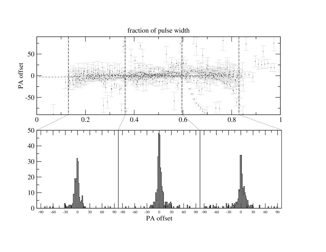
Figure 3: Top panel: The difference in PA between 1.375 and 3.1 GHz, as a function of the position within the width of the pulse, where PA measurements are possible.

5 Discussion

Of the pulsars studied here, only Vela, PSRs J0742-2822, J1056-6258 and J1359-6038 show a smooth, unbroken PA swing expected under the RVM. RVM fitting can be performed with confidence only in the former two cases. For 10 of the pulsars in our list, $\alpha$ has been derived in Rankin (1993a, b), by using the width of the central component. The derived values are mostly in agreement with geometrical values presented by Lyne & Manchester (1988), who instead made use of the RVM. However, as is typical of the pulsar population generally (especially at high frequencies), computing geometrical parameters such as $\alpha$ and $\beta$ must necessarily be subject to large uncertainties. We therefore do not concentrate on the geometrical implications of these results; rather we focus on possible causes of PA variations and their frequency dependence based purely on a direct comparison between the PA curves. We have made note of observations at other frequencies but caution that observations made with low time resolution can often be misleading.

We do note however, that many of the pulsars in our sample show complex (multi-component) profiles and large overall PA swings. This likely indicates that $\beta$ is small in these pulsars and the sightline traverses close to the magnetic pole. Also, deviations of the PA from smooth RVM curves tend to occur mostly in the centre of profiles either because components overlap there or perhaps for some physical reason assoicated with core emission. Observations at even higher frequencies, where individual components are narrower and the core emission much less prominent would then reveal smoother PA curves, an effect which is seen, at least in some pulsars (von Hoensbroech et al., 1998).

The 17 pulsars presented in Figures 1 and 2 and described in the previous section demonstrate the diversity in emission properties. The number of total intensity components, the degree of polarisation and the swing of the PA with pulse longitude vary significantly from pulsar to pulsar. Superposing the pulse profiles at 1.375 and 3.1 GHz reveals differences in the emission properties between these two frequencies. These differences, noted in the previous section, mostly relate to the ratios of the various component amplitudes within a profile and the varying degree of linear and circular polarisation of individual components at the two frequencies. The changing component amplitude ratios are a manifestation of the different spectral behaviour of different components, a topic extensively discussed recently by Karastergiou et al. (2005).

The pulse widths presented in Table 1 reveal little change between 1.375 and 3.1 GHz. This is not surprising, considering that both these frequencies are relatively high. The flaring of the last open magnetic field lines that results in broader profiles at lower frequencies does not appear to play a significant role here. Mitra & Rankin (2002) also point out that components that originate from magnetic field lines closer to the magnetic axis have the same widths across wider frequency ranges. It is therefore evident that information on the difference in emission heights cannot be gleaned from the pulse widths. For the pulsars of Figure 2, namely J1056$-$6258 and J1359$-$6038, the PA alignment method may not be accurate, due to intrinsic PA changes. For the remaining pulsars we observed, the PA method aligns the profiles to $\pm 1$ data bin, the sampling time of which is equal to the pulse period over 1024. This places a limit on the range of emission height differences between 1.375 and 3.1 GHz for our pulsars, ranging from $\sim 6.7$ km for the Vela pulsar to $\sim 64.8$ km for J1602$-$5100, as computed from Equation 5.

There are also 4 pulsars in our source list (PSRs 0942$-$5552, 1157$-$6224, 1356$-$6230 and 1807$-$0847) that have profiles with an outer component pair flanking a central component. In all 4, the relative intensity of the outer components with respect to the central component is higher at 3.1 than at 1.375 GHz. However, none of these sources show spectacular effects when it comes to the PA evolution with frequency. In fact, the first three pulsars show flat PAs across the central component at both frequencies and only PSR J1807$-$0847 has a steep PA swing in the middle of the profile. Unfortunately, however, the linear polarisation is very low in the central component of this pulsar, making the frequency comparison close to impossible.

For these 4 pulsars it is possible to derive absolute emission heights at each frequency, just by measuring the offset of the central peak from the middle of the outer components (Gangadhara & Gupta, 2001; Dyks et al., 2004). Although the direction of the offset is in agreement with the fact that the central component is emitted at a lower height (the leading outer component is always closer to the central component than its trailing counterpart), it is clear that the offset is identical at the two frequencies for all 4 of the aforementioned pulsars. This constitutes further evidence that the emission heights are very similar between the two observed frequencies. The absolute emission heights derived, using equation 7 of Dyks et al. (2004), are 14.5, 80, 33.5 and 4.5 km respectively for the aforementioned 4 pulsars. PSR 1807$-$6230 has the shortest rotation period from this selection, limiting the radius of its magnetosphere.

In the PA profiles, there is an obvious overall similarity between the two frequencies. Occasionally, the PA is different in narrow or extended parts of the profile, although even then, the agreement between frequencies outweighs the disagreement. To illustrate this, we have summarised in Figure 3 the PA differences $d$PA in all the pulsars we observed. We initially identified the pulse widths over which PA measurements were possible, for all the pulsars. The abscissae on the top panel denote the pulse longitude as a fraction of this width. Note that these widths are sometimes greater than the W₁₀ widths of Table 1. This creates a normalised pulse longitude scale for all the pulsars. The points on the plot represent the difference in PA, or $d$PA, as shown in the plots of Figures 1 and 2, plotted against their location within the pulse. Furthermore, the second panel in Figure 3 shows the histograms of $d$PA in each of three regions of the top panel. The intention is to demonstrate that the distribution of $d$PA does not obviously depend on the location within the pulse. The standard deviation of all the $d$PA values in the top panel is $16.6\degr$, compared to $13.9\degr$, $13.8\degr$ and $21.2\degr$ in the three regions of the bottom panel. The higher standard deviation value of the third region is partially caused by the large negative $d$PA values in PSR J1644$-$4559. The average error in $d$PA is $\sim 7$, so the standard deviations measured are between 2 and 3 times this value, which consolidates the observation that the PA differences cannot merely be put down to noise.

The histograms in the bottom row of Figure 3 can be used to identify OPM as a possible source of PA disagreement between 1.375 and 3.1 GHz. If at some intermediate frequency, the dominant mode of polarisation has changed, the PA at the high frequency will be orthogonal to the low frequency. Interestingly, in Figure 3 there appears to be a Gaussian spread of $d$PA around its mean of zero. The instances of $d$PA close to $90\degr$ or $-90\degr$ are few and do not represent a clear sub-group of the $d$PA distributions. This fact suggests that for our sample of sources, changes in the dominant OPM are not common between these two frequencies. The general decrease in the linear polarisation, however, is an indication that the strengths of the OPMs are becoming more equal (Karastergiou et al., 2002).

The measured standard deviation in the distribution of $d$PA places constraints on the frequency dependence of possible mechanisms that set the PA. If the superposed modes of polarisation are not orthogonal and have different spectral behaviour, a dependence of the PA on frequency will arise. The different spectral behaviour is evident by the change in linear polarisation between the two frequencies. The left plot in Figure 4 shows the effect of superposed, non-orthogonal modes of polarisation on the observed degree of linear polarisation and PA. From left to right, the lines correspond to a deviation from orthogonality of $1\degr$, $3\degr$, $5\degr$, $10\degr$ and $20\degr$. The vertical line has a length of $13\degr$, as a measure of the standard deviation of $d$PA. This figure demonstrates how large $d$PAs combined with small changes in the degree of linear polarisation, require larger departures from orthogonality of the polarisation modes. It also demonstrates that non-orthogonality of the modes results in the minimum degree of linear polarisation not being zero, as would be the case with orthogonal modes. More importantly however, this figure shows that in cases where the degree of linear polarisation changes significantly from one to the other frequency, non-orthogonality will lead to larger values of $d$PA. We conducted the following test: for all bins where the fractional linear polarisation is greater than 0.5 at 1.375 GHz, we measure the difference of the degree of linear polarisation and $d$PA between the two frequencies. The results are shown in the right plot of Figure 4. There is a hint that the points which correspond to a large change in the fractional linear polarisation, also correspond to larger $d$PA. The correlation however is very weak, which demonstrates that an explanation involving non-orthogonal polarisation modes is unlikely.

In the individual plots of Figures 1 and 2, we identify two types of deviation of $d$PA from zero. The first consists of a part of the profile where the PAs at the two different frequencies deviate in a quasi-random way, resulting in a variable $d$PA which gradually returns to zero. Good examples of this behaviour are PSRs J1243$-$6423 and J1327$-$6222. In the second type $d$PA has a constant but non-zero value across a fraction of the pulse profile. The PAs at 1.375 and 3.1 GHz run parallel to each other and then converge to being identical. Examples of this can be found in PSRs J0738$-$4042 and J1644$-$4559.

In the pulsars that belong to the first type, the total power profiles are complex with generally low linear polarisation. We can often discern what appear to be several, partially overlapping components of linear polarisation, coinciding with the most perturbed parts of the PA swing. The question then arises whether the observed changes in PA are merely due to changes in the relative strengths of overlapping components of linear polarisation. It seems appropriate to conduct such tests for PSRs J1243$-$6423 and J1327$-$6222, to formulate a model. From our data, the ratios of the various components in e.g. PSR J1243$-$6423 are certainly different at 1.375 and 3.1 GHz, however single pulse data is required to properly account for the effects of superposed modes of polarisation (Karastergiou et al., 2003). Also, in the case of the Vela pulsar where the linear polarisation is very high, the second component in the leading edge of the profile becomes more prominent at 3.1 GHz and at the same time the PA profile is distorted at the same pulse longitudes. An interpretation based on overlapping components with intrinsically different PAs again seems likely.

For the second type of $d$PA offsets, the same reasoning cannot explain the observations. It is tempting to attribute the fact that some components show a constant offset in PA between 1.375 and 3.1 GHz, e.g. the leading component of PSR J0738$-$4042, to a different Faraday Rotation measure. Although we cannot rule this possibility out, there seems to be little support in terms of the underlying physics. However, a proper test requires one more observing frequency, to check if the dependence of PA on frequency is of the same nature as Faraday Rotation. The fact that the observed difference in PA corresponds only to a few units of rotation measure does not permit us to conduct this test within one of the bands of observation.

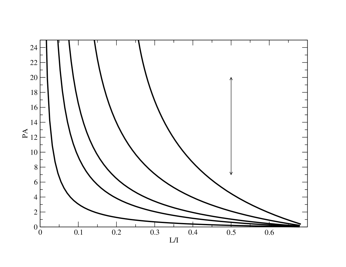
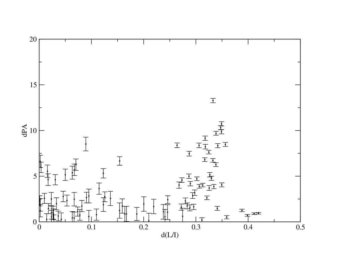
Figure 4: Left: The effect of superposed, non-orthogonal polarisation modes on the observed PA and degree of linear polarisation (L/I). The different curves, from left to right, correspond to a deviation from orthogonality of $1\degr$, $3\degr$, $5\degr$, $10\degr$ and $20\degr$. Right: $|d$PA$|$ plotted against the difference in the fractional linear polarisation, for all instances of high linear polarisation at 1.375 GHz.

6 Conclusions

We have presented for the first time superposed polarimetric profiles of 17 pulsars at 1.375 and 3.1 GHz, with absolute values of PA. The presentation demonstrates the frequency dependence of the PA as a function of pulse longitude. We find that, in general:

• The PA profiles are similar at the two frequencies, despite the lack of resemblance to the RVM curve.

• We can identify a tentative association between the changes in the PA between 1.375 and 3.1 GHz and the change in relative amplitude of overlapping total power components. This observation clashes with the RVM in that the polarization of the emission at each pulse longitude is constrained by the pulse component in which it belongs, rather than being determined purely by geometry.

• The similarities permit an alignment method based on the PA profile, which allows us to calculate very accurate RMs. The method performs very well for all but two pulsars: J1056$-$6258 and J1359$-$6038, where an explanation related to intrinsic development of the PA profile seems more likely.

• In our sample, there are not many instances of the PA at one frequency being orthogonal to the other.

• Using our measurements of the fractional linear polarisation, we place constraints on the degree of non-orthogonality between the polarisation modes.

• Although in most pulsars the differences in PA between the two frequencies vary on short scales of pulse longitude, in some pulsars such as J0738$-$4042, we have found a constant offset in PA across extended parts of the profile. We intend to perform specific observations on this pulsar to identify whether this offset can be accounted for by a different RM value, or some other physical effect.

References

- Backer & Rankin (1980) Backer D. C., Rankin J. M., 1980, ApJS, 42, 143
- Backer et al. (1975) Backer D. C., Rankin J. M., Campbell D. B., 1975, ApJ, 197, 481
- Blaskiewicz et al. (1991) Blaskiewicz M., Cordes J. M., Wasserman I., 1991, ApJ, 370, 643
- Cordes (1978) Cordes J. M., 1978, ApJ, 222, 1006
- Cordes et al. (1978) Cordes J. M., Rankin J. M., Backer D. C., 1978, ApJ, 223, 961
- Costa et al. (1991) Costa M. E., McCulloch P. M., Hamilton P. A., 1991, MNRAS, 252, 13
- Dyks et al. (2004) Dyks J., Rudak B., Harding A. K., 2004, ApJ, 607, 939
- Everett & Weisberg (2001) Everett J. E., Weisberg J. M., 2001, ApJ, 553, 341
- Gangadhara & Gupta (2001) Gangadhara R. T., Gupta Y., 2001, ApJ, 555, 31
- Gould & Lyne (1998) Gould D. M., Lyne A. G., 1998, MNRAS, 301, 235
- Hamilton & Lyne (1987) Hamilton P. A., Lyne A. G., 1987, MNRAS, 224, 1073
- Hamilton et al. (1977) Hamilton P. A., McCulloch P. M., Ables J. G., Komesaroff M. M., 1977, MNRAS, 180, 1
- Hamilton et al. (1977) Hamilton P. A., McCulloch P. M., Manchester R. N., Ables J. G., Komesaroff M. M., 1977, Nature, 265, 224
- Han et al. (1999) Han J. L., Manchester R. N., Qiao G. J., 1999, MNRAS, 306, 371
- Hotan et al. (2004) Hotan A. W., van Straten W., Manchester R. N., 2004, Publications of the Astronomical Society of Australia, 21, 302
- Karastergiou & Johnston (2004) Karastergiou A., Johnston S., 2004, MNRAS, 352, 689
- Karastergiou et al. (2003) Karastergiou A., Johnston S., Kramer M., 2003, A&A, 404, 325
- Karastergiou et al. (2005) Karastergiou A., Johnston S., Manchester R. N., 2005, MNRAS, pp 285–+
- Karastergiou et al. (2003) Karastergiou A., Johnston S., Mitra D., van Leeuwen A. G. J., Edwards R. T., 2003, MNRAS, 344, L69
- Karastergiou et al. (2002) Karastergiou A., Kramer M., Johnston S., Lyne A. G., Bhat N. D. R., Gupta Y., 2002, A&A, 391, 247
- Kramer (1994) Kramer M., 1994, A&AS, 107, 527
- Lyne & Manchester (1988) Lyne A. G., Manchester R. N., 1988, MNRAS, 234, 477
- McCulloch et al. (1978) McCulloch P. M., Hamilton P. A., Manchester R. N., Ables J. G., 1978, MNRAS, 183, 645
- Malov & Suleimanova (1998) Malov I. F., Suleimanova S. A., 1998, Astronomy Reports, 42, 388
- Manchester et al. (1980) Manchester R. N., Hamilton P. A., McCulloch P. M., 1980, MNRAS, 192, 153
- Manchester et al. (1975) Manchester R. N., Taylor J. H., Huguenin G. R., 1975, ApJ, 196, 83
- Melrose (2000) Melrose D. B., 2000, in Kramer M., Wex N., Wielebinski R., eds, Pulsar Astronomy - 2000 and Beyond, IAU Colloquium 177 The status of pulsar emission theory. Astronomical Society of the Pacific, San Francisco, p. 721
- Michel (1991) Michel F. C., 1991, Theory of Neutron Star Magnetospheres. University of Chicago Press, Chicago
- Mitra & Li (2004) Mitra D., Li X. H., 2004, A&A, 421, 215
- Mitra & Rankin (2002) Mitra D., Rankin J. M., 2002, ApJ, pp 322–336
- Radhakrishnan & Cooke (1969) Radhakrishnan V., Cooke D. J., 1969, ApL, 3, 225
- Ramachandran et al. (2004) Ramachandran R., Backer D. C., Rankin J. M., Weisberg J. M., Devine K. E., 2004, ApJ, 606, 1167
- Rankin (1986) Rankin J. M., 1986, ApJ, 301, 901
- Rankin (1993a) Rankin J. M., 1993a, ApJ, 405, 285
- Rankin (1993b) Rankin J. M., 1993b, ApJS, 85, 145
- Ruderman & Sutherland (1975) Ruderman M. A., Sutherland P. G., 1975, ApJ, 196, 51
- Stinebring et al. (1984) Stinebring D. R., Cordes J. M., Rankin J. M., Weisberg J. M., Boriakoff V., 1984, ApJS, 55, 247
- Taylor et al. (1993) Taylor J. H., Manchester R. N., Lyne A. G., 1993, ApJS, 88, 529
- van Ommen et al. (1997) van Ommen T. D., D’Alesssandro F. D., Hamilton P. A., McCulloch P. M., 1997, MNRAS, 287, 307
- von Hoensbroech et al. (1998) von Hoensbroech A., Kijak J., Krawczyk A., 1998, A&A, 334, 571
- von Hoensbroech & Xilouris (1997a) von Hoensbroech A., Xilouris K. M., 1997a, A&A, 324, 981
- von Hoensbroech & Xilouris (1997b) von Hoensbroech A., Xilouris K. M., 1997b, A&AS, 126, 121