Star Formation Rates and Extinction Properties of IR-Luminous Galaxies in the Spitzer First Look Survey

Abstract

We investigate the instantaneous star formation rates ($SFR$) and extinction properties for a large ($N=274$), near-infrared (NIR: 2.2µm) + mid-infrared (MIR: 24µm) selected sample of normal to ultra-luminous infrared galaxies (ULIRGs) [$10^{9}<L_{IR}/L_{\odot}<10^{12.5}$] with $\langle z\rangle\sim 0.8$ in the Spitzer Extragalactic First Look Survey (FLS). We combine Spitzer MIPS 24µm  observations with high-resolution, optical Keck Deimos spectroscopy to derive optical emission-line ($H\alpha$, $H\beta$, [OII]) and infrared star formation rates ($SFR_{opt}$ & $SFR_{IR}$, respectively). Direct comparison of these SFR diagnostics reveals that our sample exhibits a wide range of extinction ($1.0<A_{v}<4.0$ mag). This is after removing spectroscopic and IRAC color-selected AGN candidates that account for $\approx\!12\%$ of the sample. Objects with SFRs of a few solar masses per year have $A_{v}$ values consistent with those of normal spirals ($A_{v}\!\approx\!1.0$ mag). By contrast, LIRGs at $z\gtrsim 1$, which make up a large fraction of our sample, have $SFR\!\approx\!100$ $M_{\odot}yr^{-1}$ and a mean $A_{v}\!\approx\!2.5$ mag. This translates to a 97% mean attenuation of the [OII] $\lambda\lambda 3727$ forbidden line doublet, with the most extreme sources having as much as 99.7% of their [OII] line flux extinguished by dust. Based on a $SFR_{IR}/SFR_{opt}$ diagnostic, we derive an IR-luminosity-dependent $A_{v}^{IR}$ function [$A_{v}^{IR}=0.75*log(L_{IR}/L_{\odot})-6.35$ mag] that we use to extinction correct our emission line luminosities. Application of this correction results in a correlation between $SFR_{IR}$ and $SFR_{opt}$ that has a dispersion of 0.2 dex (Semi-Interquartile Range). Investigation of the $A_{v}$ dependence on redshift reveals that for a fixed $L_{IR}$ there is no significant $A_{v}$ evolution. Comparisons to previous studies reveal that the mean attenuation of our sample is intermediate between that of local optical/UV- and radio-selected samples and has a marginally stronger $L_{IR}$ dependence.

1. Introduction

Numerous investigations over the past decade have been directed at measuring the cosmic star formation history (SFH) of the Universe. Observations over the full spectrum from radio to X-ray have been exploited to trace star formation rates (see Kennicutt, 1998; Condon, 1992; Ghosh & White, 2001, for reviews of the various diagnostics). The most commonly utilized have historically been $H\alpha$ and [OII] emission line and UV continuum flux (eg. Madau et al., 1996; Tresse & Maddox, 1998; Hogg et al., 1998; Yan et al., 1999; Glazebrook et al., 1999; Adelberger & Steidel, 2000; Erb et al., 2003). This is largely due to their respective accessibility via ground-based observing windows for local and distant samples and the fact that they are relatively direct tracers of massive star formation. Unfortunately, optical and UV diagnostics are highly sensitive to dust attenuation. Various approaches have been implemented to estimate this reddening. The use of Balmer line flux ratios is a direct, but observationally taxing method that requires high resolution spectroscopy. In the absence of multiple well measured emission lines, color- or magnitude-dependent optical extinction corrections (Rigopoulou et al., 2000; Hippelein et al., 2003), or the UV slope-extinction relation [$\beta$-$A_{UV}$] derived for starburst galaxies (eg. Calzetti et al., 1994; Adelberger & Steidel, 2000) have also been adopted. Though commonly applied to non-starburst galaxies, the latter has been shown to break down for both more and less luminous systems (Goldader et al., 2002; Bell et al., 2002; Bell, 2002).

By comparison, far-infrared (FIR) and radio star formation rate (SFR) diagnostics have the advantage that they are unaffected by extinction. Their shortcoming, however, is that for general populations they have more complex relationships to the star formation than optical emission line and UV indicators. For instance, the typically adopted FIR SFR calibration (Kennicutt, 1998) is based on the assumption of infinite optical depth and 100% reprocessing of massive star UV emission into IR flux. This is a reasonable assumption for heavily extinguished systems, but breaks down for galaxies with moderate attenuation. In spiral galaxies for instance, counteracting effects of UV radiation leakage and heating from older evolved stellar populations must also be considered (Lonsdale-Persson & Helou, 1987). Finally, despite our relatively limited understanding of the decimeter radio continuum, it has served as a powerful proxy for the IR flux due to the tightness of radio-FIR correlation (Helou et al., 1985). Surprisingly, this correlation extends to IR luminosities ($\approx\!0.01$ L*) at which neither the bolometric infrared luminosity ($L_{IR}$) nor the radio continuum are reliably tracing star formation (Bell, 2003).

Comparative studies of these different diagnostics exist for a range of galaxy types and sample selections. UV and $H\alpha$ measurements have been found to be generally consistent for local samples of normal galaxies (Sullivan et al., 2001; Bell & Kennicutt, 2001; Buat et al., 2002; Sullivan et al., 2004). The scatter and, in some cases, the offset between the tracers are primarily attributed to a combination of uncertainties in the extinction correction, star/dust geometry and the star formation timescale (Helou & Bicay, 1993; Bell, 2003; Sullivan et al., 2004). The inter-comparison of UV/optical to decimeter radio emission (Sullivan et al., 2001; Afonso et al., 2003) and far-infrared IRAS observations (Cram et al., 1998; Dopita et al., 2002; Kewley et al., 2002; Hopkins et al., 2003) for large local samples confirms the importance of accurate UV/optical attenuation corrections. Recent ISO-based studies by Rigopoulou et al. (2000),Cardiel et al. (2003) and Flores et al. (2004) probe out to more distant redshifts ($z\sim 1$) but for admittedly small samples of 12, 7 and 16 sources, respectively. These pioneering works provide the deepest IR-based SFR probes of the distant, dustier and more actively starforming universe. Consequently, they tend to include more extreme, IR luminous galaxies than are present in the local samples.

Due to the absence of a unified multiwavelength picture of the SFH, there is considerable debate about the star formation density at high redshift. Most controversy revolves around issues of sample selection effects, SFR calibration uncertainties and dust attenuation corrections. It has become clear that no single tracer is applicable for all galaxies. UV & optical diagnostics appear to be well suited for low IR luminosity galaxies that do not require significant extinction corrections; whereas attenuation-free IR and radio diagnostics provide better estimates in dusty, actively starforming systems. In this work we study the star formation and extinction properties of a large, distant, actively starforming population by making a direct comparison of optical emission line and IR SFR diagnostics. Specifically, we use mid-IR observations from the Spitzer Extragalactic First Look Survey and deep Keck optical spectroscopic observations to achieve an order of magnitude increase in sample size over previous high redshift ISO studies.

This paper is divided into the following sections. A summary of the various observational components and their basic analysis is given in §2. Calculations of the optical and infrared star formation rates are described in §3. Our approach for removing contaminating AGN is outlined in §4. The comparison between the optical and IR SFRs and our derived extinction corrections are discussed in §5. The main points of this work are summarized in §6. Throughout the paper, we adopt the cosmology of $\Omega_{m}=0.27$, $\Omega_{\Lambda}=0.73$ and $H_{\circ}=70$ km s^-1 Mpc^-1.

2. Observations and Reductions

The Spitzer Extra-galactic First Look Survey (FLS) region is a $\approx\!4$ sq. deg region centered around RA=$17^{h}18^{m}00^{s}$, Dec=$59^{\circ}30^{\prime}00^{\prime\prime}$. It is chosen to lie within the continuous viewing zone (CVZ), have minimum cirrus and no bright radio sources. Observations of this field with each of the 4 IRAC and 3 MIPS imaging bands was one of the first science tasks undertaken by Spitzer. In addition to IR imaging, numerous ancillary datasets including radio, optical and near-IR (NIR) data have been taken in this field. Brief descriptions of the datasets included in this study are given below.

2.1. Imaging

2.1.1 Optical

Optical $R$-band imaging of the FLS was carried out using the MOSAIC-I camera on the 4-meter Mayall Telescope at the Kitt Peak National Observatory on four consecutive nights on UT 2000 May 4-7. A $4\times 2$ array of SITe $2048\times 4096$ CCDs provides a $36^{\prime}\times 36^{\prime}$ field of view with a $0.258^{\prime\prime}$ pixel scale. Tiling 26 individual pointings we obtain an $R$-band coverage of 9.4 sq. deg, with median exposure time per pointing of 1800 sec and typical seeing FWHM$\sim\!1.0^{\prime\prime}$. The resulting source catalog has a 50% completeness limit of $R=24.5$ mag (Vega). In addition, $g\arcmin$ & $i\arcmin$-band observations of the FLS were obtained using the Large Format Camera (LFC) on the 200-inch Palomar Observatory Hale Telescope. These observations were taken over multiple observing campaigns from August 2001 through June 2004. The total area coverage in these bands is roughly 2.0 sq. deg, with comparable seeing and resolution to that of the $R$-band data. Comprehensive descriptions of these datasets are presented in  Fadda et al. (2004) and Glassman et al. (2005, in preparation).

2.1.2 Near-infrared

Near-infrared observations were carried out in two separate, but complimentary observing campaigns that can be characterized as shallow, wide-field and deep, narrow-field. In the first, $K_{s}$-band imaging of a 1.14 sq. deg region, to a median depth of $K_{s}<19.0$ mag (Vega) was performed on UT 2001 May 23-26 using the Florida Multi-object Imaging Near-IR Grism Observational Spectrometer (FLAMINGOS) on the Kitt Peak National Observatory 2.1-m telescope. A $2048\times 2048$ HgCdTe Rockwell array provides a $20^{\prime}\times 20^{\prime}$ field of view with $0.6^{\prime\prime}$ pixel scale. Each pointing was comprised of 50, 30-sec exposures taken in a 25-position dither pattern. The field was mapped with a $5\times 5$ grid pattern using half-field offsets ($10^{\prime}$) between pointings. The median exposure time is 2400 sec per pixel, and the median stellar PSF over the mosaic is FWHM=$1.6^{\prime\prime}$.

In addition to the KPNO dataset, a smaller $\approx\!45^{\prime}\times 45^{\prime}$ verification region in the center of the FLS was observed with the Wide-field Infrared Camera (WIRC) on the Palomar Observatory Hale 200-inch telescope. Observations were undertaken over the course of multiple observing runs between June 2002 and July 2004. A $2048\times 2048$ Hawaii-II HgCdTe array provides a $8.7^{\prime}\times 8.7^{\prime}$ field of view with a $0.25^{\prime\prime}$ pixel scale. The $\approx\!0.6$ sq. deg area centered on the FLS verification region was covered with 34 tiled pointings. The average exposure time per pointing is 3600 sec ($120\times 30$sec) taken with a 30-position random dither pattern, to a median depth of $K_{s}<20.2$ mag (Vega). A detailed description of all of the NIR observations and reductions is presented in Glassman et al. (2005, in preparation).

2.1.3 Mid-Infrared

The extragalactic component of the Spitzer FLS is comprised of Infrared Array Camera (IRAC) (Fazio et al., 2004) and Multiband Imaging Photometer for Spitzer (MIPS) (Rieke et al., 2004) observations taken in December 2003 with a total exposure time of 63 hours. The MIPS 24µm  area coverage was 4.4 sq. deg for the main field and 0.26 sq. deg in a deeper verification field, with respective 3$\sigma$ depths of $0.11/0.08$ mJy. All data were processed and stacked by the data processing pipeline at the Spitzer Science Center (SSC). MIPS photometry was performed using StarFinder Diolaiti et al. (2000), which measures profile-fitted fluxes for point sources. A complete description of the 24µm  data reduction and source catalog can be found in Marleau et al. (2004) and Fadda et al. (2005, in preparation).

2.2. Spectroscopy

Optical spectroscopy was obtained with the Deep Imaging Multi-Object Spectrograph (DEIMOS; Faber et al., 2003) on the W. M. Keck II 10-meter telescope. Observations were performed over 3 nights from UT 2003 June 27-29. A 1200 line mm^-1 grating with central wavelength settings of 7400Å  and 7699Å  was used with the GG495 blocking filter, resulting in a 0.33Å  pix^-1 mean spectral dispersion and a 1.45Å  instrumental resolution. The total spectral range observed was $6300-9300$Å; however, the coverage for an individual source was limited to 2,630Å  with a slit position dependent starting wavelength.

A total of 14 multi-slit masks were observed, with $\approx\!100$ $1^{\prime\prime}$ wide slits per mask. The $5^{\prime}\times 16^{\prime}$ slitmasks were tiled in 11 unique positions to sample a $25^{\prime}\times 45^{\prime}$ area centered on the FLS. In Figure 1, mask positions are shown on top of the 24µm  mosaic for illustration. Multiple masks were observed for three of the positions in the deepest central region. Table 1 lists the positions, PAs and exposure times for the 14 observed masks.

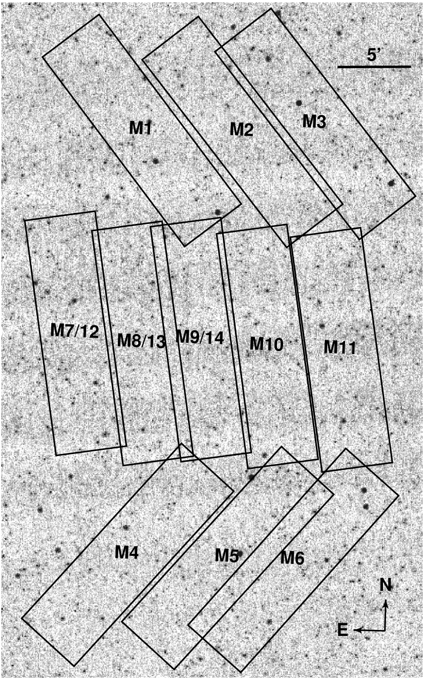
Figure 1.— MIPS 24µm  image of the central $30^{\prime}\times 45^{\prime}$ region of the First Look Survey Verification region. Positions of 14 $5^{\prime}\times 17^{\prime}$ Keck Deimos optical spectroscopy slitmasks are shown. A summary of the spectroscopic observations is given in Table 1.

Table 1Spectroscopic Observation Log

ID	RA (J2000)	Dec (J2000)	P.A. (deg)	Exposure Time
M1	17:17:08.51	59:59:53.5	-39	$3\times 20$ min
M2	17:16:11.74	60:00:02.3	-40	$3\times 20$ min
M3	17:15:30.86	60:00:46.0	-40	$3\times 20$ min
M4	17:17:07.65	59:29:58.6	40	$3\times 20$ min
M5	17:16:12.00	59:30:00.0	40	$3\times 20$ min
M6	17:15:35.57	59:29:58.8	39	$3\times 20$ min
M7	17:17:41.53	59:45:26.1	-10	$5\times 45$ min
M8	17:17:03.68	59:45:00.0	-10	$4\times 45$ min
M9	17:16:31.14	59:45:24.8	-10	$4\times 45$ min
M10	17:15:53.81	59:45:05.2	-10	$3\times 20$ min
M11	17:15:12.35	59:45:00.6	-10	$3\times 20$ min
M12	17:17:41.39	59:45:32.0	-10	$3\times 20$ min
M13	17:17:03.68	59:45:00.0	-10	$3\times 20$ min
M14	17:16:31.14	59:45:24.8	-10	$3\times 20$ min

We require minimum slit lengths of $7^{\prime\prime}$ for local sky subtraction and adopt the DEEP2 recommended strategy of using tilted slits to better sample and remove sky lines. Slit position angles $\theta$ were required to be $10<|\theta|<25$ degrees from the spatial axis and when possible, were positioned along the major axis of elongated galaxies. Of the 14 masks, 3 were observed for a total of 10,800 sec ($3\times 3600$sec) and the remaining 10 masks were observed for a total of 3,600 sec ($3\times 1200$sec). Observing conditions over the course of the run were good, with typical seeing FWHM$\sim\!0.7^{\prime\prime}$. For data reduction, we employ the DEEP2 spec2d pipeline, which is based on the SDSS spectral reduction package. This package performs cosmic ray removal, flat-fielding, co-addition, sky subtraction, wavelength calibration and both 2-d and 1-d spectral extraction.

2.2.1 Emission-line measurements and Redshift Identification

The 1-d spectral output of the DEEP2 pipeline are analyzed using an in-house IDL package written by PIC & DF. Galaxy redshifts are identified through visual inspection and galaxy template cross correlation. Line flux, equivalent width and kinematic measurements are made by performing Gaussian profile fits to the 1-d spectra. This is done interactively with the user identifying the lines to be fit and specifying the spectral region over which to perform the line+continuum fit. Our high spectral resolution (1.45Å  instrumental resolution) allows for most lines to be modeled individually. One exception is the [OII] doublet $\lambda\lambda 3726,3729$, which is unresolved in $\approx\!1/2$ of our sample. Rather than measure each line independently, we adopt a double Gaussian profile with a fixed line separation of [$(1+z)\times 2.75$Å]. We require the two lines to have the same FWHM, but allow their flux ratio to be a free parameter.

In the case of Balmer line fits, two-component emission+absorption profiles are adopted. It is well known that nebular Balmer emission lines can suffer from contamination due to underlying stellar absorption and subsequently be underestimated. The standard technique to correct for stellar absorption is to apply a global Balmer line equivalent width correction. Fortunately, our high spectral resolution enables us to resolve and directly measure the nebular emission and the pressure broadened stellar absorption components. This eliminates the need for a global correction and results in more accurate line fluxes. Figure 2 provides an illustration of two typical emission line fits. Figure 2a shows a double Gaussian line fit to the [OII] $\lambda\lambda 3727$ doublet, while Figure 2b shows an emission+absorption two-component fit to $H\beta$.

Figure 2.— Line fits of [OII] and $H\beta$ for two representative objects in our sample. In panel (a), the [OII] $\lambda\lambda 3727$ doublet is shown. The gaussian profiles of the individual lines (dotted) are shown along with their co-addition (dashed). The lines are required to have the same FWHM and a fixed 2.75Å  restframe separation. In panel (b), individual components (dotted) and the coadded $H\beta$ line-fit (dashed) are shown.

2.2.2 Final MIR+NIR Sample

The spectroscopic observations were designed to target a flux-limited NIR-selected sample based primarily on our $K_{s}$-band dataset. Optical $g\arcmin$-, $R$- & $i\arcmin$-band color information was included exclusively to a) clean out stellar contaminants and b) apply a rough photometric redshift selection, designed to prioritize high redshift sources with $z>0.6$. The detailed description of this color selection will be discussed separately in the spectroscopic catalog paper.

The final sample used for this study includes all galaxies in our spectroscopic sample with a high confidence redshift and a significant 24µm  detection. In Figure 3, the full NIR-selected sample with good spectroscopic redshifts (solid) is shown in contrast to the subsample that have 24µm-detected counterparts (dashed).

The effect of our $g\arcmin,R,i\arcmin,K_{s}$ color selection is seen in both distributions as a sharp dropoff below $z<0.6$. Beyond $z>1.1$ the impact of our decreasing spectroscopic redshift sensitivity is evident. In this regime strong sky lines make it challenging to cleanly identify [OII] $\lambda\lambda 3726,3729$. By $z>1.3$, this feature has moved out of our spectral coverage window for much of our sample. The final $K_{s}$+24µm  sample includes 274 galaxies and has a median redshift of $\tilde{z}=0.76$.

To investigate how our spectroscopic redshift target selection is biasing our NIR+MIR distribution, we show in Figure 4, the $K_{s}$ versus 24µm  flux for the parent photometric sample (dots) and the targeted spectroscopic sample (crosses). Our selection against low redshift sources is evident in this distribution by the lack of NIR bright ($K_{s}<16.5$ mag) spectroscopic targets.

Figure 3.— Spectroscopic redshift distribution of our full 676 galaxy sample (solid) and the 274 galaxy, 24µm-detected subsample (dashed).

Figure 4.— MIPS 24µm  flux versus $K_{s}$-band mag for the spectroscopic (crosses) and parent photometric (dots) samples. Comparison of the two distributions illustrates that the parent population is being reasonably well represented with our spectroscopic sample for all but the brightest sources ($K_{s}>16.5$ mag).

3. SFR Computations

3.1. Emission-Line SFR diagnostics

The $H\alpha$ $\lambda 6563$ emission line is the most prominent and often measured SFR diagnostic in local galaxy surveys. Unfortunately, at even moderate redshifts ($z\gtrsim 0.4$), this line becomes observationally taxing as it moves first into the forest of OH sky lines and then beyond the optical spectral window. Higher order Balmer lines such as $H\beta$ and $H\gamma$ can be related to $H\alpha$; however, these are often overlooked because their weak line strength and contamination from underlying stellar absorption make them difficult to measure. At redshifts where all the prominent Balmer lines become inaccessible ($z\gtrsim 0.9$), the [OII] doublet $\lambda\lambda 3727$ can be used based on the $H\alpha$/[OII] line ratio. For this study, we use a combination of all these lines to track the SFR over the redshift range of our sample. $H\alpha$, $H\beta$ and [OII] are measured for galaxies in the respective redshift ranges $z\lesssim 0.4$, $0.3\gtrsim z\gtrsim 0.9$, and $z\gtrsim 0.7$. When accessible, $H\gamma$ and $H\delta$ are also used as secondary diagnostics. In this section, we discuss the flux measurement and SFR conversion for each of these lines.

3.1.1 Line Luminosity Measurement

The most direct approach for measuring the total emission line flux of a galaxy is direct integration of a flux-calibrated spectrum. Unfortunately, this is impractical for many surveys, given the challenges of properly flux calibrating large multi-slit samples. An alternate route is to combine line equivalent widths with broadband photometry (eg. Hogg, Cohen, Blandford, & Pahre, 1998; Hopkins, Miller, Nichol, Connolly, Bernardi, Gómez, Goto, Tremonti, Brinkmann, Ivezić, & Lamb, 2003). In our case, we compute $k$-corrected absolute $u\arcmin$,$g\arcmin$ & $R$-band magnitudes using our observed $g\arcmin$,$R$, $i\arcmin$ and $K_{s}$ photometry and the KCORRECT code (Blanton et al., 2003), adapted for our dataset. We adopt these restframe magnitudes as approximations of the continuum flux density at the rest wavelengths of [OII], $H\beta$ and $H\alpha$ (3727Å, 4861Å and 6563Å, respectively). Luminosities of these emission lines are then given by:

$$L_{H{\alpha}}=EW_{H{\alpha}}10^{[-0.4(M_{R}-34.10)]}\frac{3.0\times 10^{18}}{\lambda_{rest}^{2}}~{}~{}~{}~{}(W)$$ (1)

$$L_{H{\beta}}=EW_{H{\beta}}10^{[-0.4(M_{g^{\prime}}-34.10)]}\frac{3.0\times 10^{18}}{\lambda_{rest}^{2}}~{}~{}~{}~{}(W)$$ (2)

$$L_{[OII]}=EW_{[OII]}10^{[-0.4(M_{u^{\prime}}-34.10)]}\frac{3.0\times 10^{18}}{\lambda_{rest}^{2}}~{}~{}~{}~{}(W)$$ (3)

where $EW$ is the line equivalent width in angstroms; $M$ is the $k$-corrected absolute AB magnitude appropriate for the rest wavelength of the line being measured; and $\lambda_{rest}$ is the central wavelength of the broadband filter, also in angstroms. These derivations assume that the continuum flux at a given emission line wavelength is well approximated by the flux density at the corresponding broadband effective wavelength. An additional color correction can be made to account for the wavelength difference between the line and the filter effective wavelength; however, we find this correction to be negligibly small (of order a few percent), so it is excluded.

A major benefit of this approach is that it alleviates the need for aperture/slit corrections that can plague direct flux measurements. These corrections are small for compact galaxies, but can be substantial for extended sources. Consequently, aperture loss tends to be redshift dependent and has the potential to masquerade as evolution. By constrast, line equivalent widths and the scaled line fluxes described above are fairly insensitive to slit loss. This approach does rely on the underlying assumption that the average line-to-continuum ratio within the slit is the same as that outside the slit; however, the same assumption is made when correcting for slit loss.

3.1.2 Balmer Line SFR diagnostics

The Balmer line star formation rate diagnostics rely on the $H\alpha$-$SFR$ calibration derived by Kennicutt (1998):

$$SFR_{H\alpha}=7.90\times 10^{-42}L_{H\alpha}E_{H\alpha}~{}~{}~{}~{}(ergs~{}s^{-1})$$ (4)

where $L_{H\alpha}$ is the measured line luminosity and $E_{H\alpha}$ is the extinction correction factor, measured at the wavelength of $H\alpha$. This correlation is based on evolutionary synthesis models assuming solar abundance, a Salpeter IMF with stellar mass limits of $0.1<M<100M_{\odot}$, and $T_{e}=10,000$ K case-B recombination. It also assumes that the escape fraction of ionizing radiation from the observed galaxy is negligible, and therefore that the nebular emission traces all of the massive star formation.

The conversion for higher order Balmer lines are derived based on the intrinsic case-B recombination line ratios. As discussed in §2.2.1, these lines tend to be less frequently adopted as SFR tracers due the difficulties of properly correcting for stellar absorption; however, Kennicutt (1992) has shown that even with the adoption of a mean correction, for strong emission line galaxies $H\beta$ can be a reliable SFR diagnostic. Incorporating the expected $H\alpha/H\beta=2.87$ line ratio (Osterbrock, 1989), we obtain the following relation for $SFR_{H\beta}$:

$$SFR_{H\beta}=2.75\times 10^{-42}L_{H\beta}E_{H\beta}~{}~{}~{}~{}(ergs~{}s^{-1})$$ (5)

where the extinction term $E_{H\beta}$ is measured at $H\beta$. Similar relations for $H\gamma$ and $H\delta$ are derived based on the $H\gamma/H\beta=0.466$ and $H\delta/H\beta=0.256$ line ratios.

3.1.3 [OII] Forbidden Line SFR diagnostic

For the most distant $z\gtrsim 0.7$ sources in our sample, we compute the SFR based on the [OII] $\lambda\lambda 3727$ forbidden line doublet, adopting the Kewley et al. (2004) calibration:

$$SFR_{[OII]}=(0.66\pm 0.17)\times 10^{-41}L_{[OII]}E_{[OII]}~{}~{}~{}~{}(ergs~{}s^{-1})$$ (6)

Following the notation above $L_{[OII]}$ is the measured line luminosity and $E_{[OII]}$ is the extinction correction factor at $\lambda 3727$. An important difference with respect to most previous [OII] calibrations is that Equation 6 does not include any assumptions about the differential reddening between $H\alpha$ and [OII] of the source. By contrast, the standard conversion of Kennicutt (1998) (cf. Gallagher, Hunter, & Bushouse, 1989; Kennicutt, 1992):

$$SFR_{[OII]}=(1.4\pm 0.4)\times 10^{-41}L_{[OII]}E_{H\alpha}~{}~{}~{}~{}(ergs~{}s^{-1})$$ (7)

requires the calibration of a mean reddening between $H\alpha$ $\lambda 6563$ and [OII] $\lambda\lambda 3727$. The assumption of an average $H\alpha$-to-[OII] reddening is reasonable for samples with a narrow range of intrinsic extinction; however, it would lead to systematic, extinction-dependent errors for more general samples with broad $E(B-V)$ distributions. Also, since the current sample has a considerably brighter mean IR luminosity than that of the Kennicutt (1992) or Gallagher et al. (1989) calibration datasets, using Equation 7 would tend to underestimate both the total [OII] extinction and star formation rate.

It is worth noting that Equation 6 ignores metallicity effects on the [OII]-to-Balmer line luminosity ratio. Kewley+04 does characterize the abundance dependence of this ratio; however, due to our lack of metallicity measurements, we use their $SFR_{[OII]}$ calibration that adopts a mean abundance value of the Nearby Field Galaxy Survey (NFGS). Though a detailed investigation of this issue is beyond the scope of this work, we can use their findings to estimate the impact of metal abundance on our derived SFRs. Over the metallicity range $8.0<log(O/H)+12<9.0$ (based on McGaugh, 1991, $R_{23}$ calibration) of the NFGS sample, Kewley et al. (2004) find that the [OII]/$H\alpha$ ratio exhibits a metallicity dependent range of $\pm 0.2$ dex. The adoption of a mean abundance introduces $\lesssim 0.08$ dex of scatter into their [OII]/$H\alpha$ correlation. We expect a comparable impact on the scatter of our $SFR_{[OII]}$ diagnostic. At that level, it does not have a significant effect on our $SFR([OII])$ or extinction uncertainties.

Finally, in Figure 5 we combine the above emission line diagnostics to look at the optically-derived, extinction-uncorrected SFR versus redshift. Comparison of the parent NIR-selected sample with the 24µm-detected subsample reveals that latter has a higher mean uncorrected $SFR_{opt}$. This not an unexpected result, since IR flux traces star formation. A bit surprising is the degree of overlap between the $SFR_{opt}$ distributions of IR-detected and non-detected sources. The fact that at any given redshift, $SFR_{opt}$ (uncorrected) provides little indication of whether a source will be IR luminous or not suggests an IR-luminosity dependent attenuation.

Figure 5.— Extinction-uncorrected emission line-derived $SFR_{opt}$ versus redshift for the full 676 galaxy, NIR-selected sample (crosses) and the subset of 274 galaxy, $K_{s}$+24µm-detected sample (circles). The integrated $SFR_{opt}$ distributions of the full (solid) and 24µm-detected (dashed) samples show that the mean $SFR_{opt}$ for IR-luminous sources is higher than that of the parent population. The lack of a clean separation between the detected and non-detected sources is an expected consequence of a $L_{IR}$-dependent optical extinction.

3.2. IR SFR Calculations

An alternative SFR tracer that is unaffected by extinction is the infrared luminosity The IR component of galaxy SEDs can be decomposed into three main dust emission components: 1) a near blackbody emission profile of a thermally heated ‘cold’ big grain (BG) dust component; 2) a near blackbody component of a stochastically heated ‘warm’ very small grain (VSG) dust; and 3) molecular polycyclic aromatic hydrocarbon (PAH) emission features (Desert et al., 1990; Dale & Helou, 2002, hereafter DH02). The primary heat sources for these dust components are stellar radiation from young stars, an older evolved stellar population and AGN.

In dusty, high-opacity systems where the dominant heat source of the IR dust radiation is young stars (ie. Starbursts and LIRGs) the IR luminosity is expected to be an excellent tracer of the instantaneous SFR. In these situations, the conversion of $L_{IR}$ to a star formation rate can be made with the calibration of Kennicutt (1998),

$$SFR_{IR}=4.5\times 10^{-44}L_{IR}(ergs~{}s^{-1})$$ (8)

where $L_{IR}$ is defined as the integrated luminosity from $8-1000\micron$. Equation 8 is based on the assumption of solar abundance, a Salpeter IMF ($0.1-100M_{\sun}$) and an optically thick dust distribution. It is consistent ($\pm 30\%$) with published calibrations of comparably selected samples (Kennicutt, 1998); however, its extension to more general galaxy populations should be made with caution. Specifically, the assumption of high optical depth places an important limitation on its application to normal spiral galaxies. Large UV/optical escape fractions, whether due to low dust opacity or dust/star geometry, will cause $SFR_{IR}$ to underestimate the true SFR. On the other hand, heating of the diffuse ISM by an older background population can contribute significantly to the IR luminosity (Lonsdale-Persson & Helou, 1987; Helou, 2000), resulting in an overestimate of the SFR. At the high IR luminosity extreme, the $SFR_{IR}$ calibration runs into the problem that many ULIRGs derive a significant fraction of their bolometric luminosity from AGN. In these systems, dust heating from a central AGN can be the dominant component of $L_{IR}$. This contribution is difficult to quantify, so it is essential to screen these sources. In §4 we discuss our approach for removing AGN from our sample.

3.2.1 Bolometric Correction

To calculate $SFR_{IR}$, we first compute the bolometric IR luminosity from our observed 24µm  observations. A standard approach for deriving $L_{IR}$ for local galaxies is to use the definition of Sanders & Mirabel (1996), based on IRAS 12, 25, 60 & 100µm  luminosities:

$$L_{IR}[8-1000\mu m]=1.8\times 10^{-14}\times 10^{26}\times$$

$$[13.48L_{\nu}(12)+5.16L_{\nu}(25)+2.58L_{\nu}(60)+L_{\nu}(100)]$$

where $L_{\nu}(\lambda)$ is in units of $L_{\sun}Hz^{-1}$ and $L_{IR}$ is in units of $L_{\sun}$. A comparable Spitzer band transformation exists (DH02); however, its application for distant galaxies is hindered by the general dearth of multi-band FIR photometry. For instance, the bulk of our FLS sample is observed, but undetected with 70 & 160µm  imaging. Fortunately, it has been shown from IRAS and ISOCAM data that the MIR alone is a reasonable tracer of $L_{IR}$ (Elbaz et al., 2002; Takeuchi et al., 2005). We exploit this finding and use our 24µm  observations, which correspond to restframe $10-24\micron\,$ over the redshift range of our sample, to derive IR luminosities.

Rather than implement a single $L_{MIR}$-to-$L_{IR}$ correlation, we take the approach of using template SEDs (Chary & Elbaz, 2001, hereafter CE01) to derive $L_{IR}$[8–1000µm] from the 24µm  fluxes. CE01 have constructed a library of 105 flux-calibrated SEDs that are single-valued in $L_{IR}$ and cover the spectral range $0.1-1000$µm. They start with model SEDs matched to a sample of local galaxies ranging from a normal spiral (M51) to a ULIRG (Arp 220) (Silva et al., 1998) and combine them with MIR ISOCAM spectra and FIR model SEDs. They then split and recombine the MIR and FIR components of these templates to create a library of SEDs that reproduce the observed correlations between the various IRAS, ISOCAM and SCUBA IR fluxes of local galaxies. We implement these templates in a manner described by Elbaz et al. (2002) as the ‘multi-template’ approach. For each galaxy in our sample, we shift the template SEDs to the redshift of that source. We choose the template that most closely reproduces the observed 24µm  flux and use its 12, 25, 60 and 100µm  integrated fluxes to compute $L_{IR}$[8–1000µm] based on Equation 3.2.1. The final distribution of $L_{IR}$ for the $K_{s}$+24µm-detected sample is shown in Figure 6. This plot of $L_{IR}$ vs. redshift reveals that our sample spans a broad range in both $L_{IR}$ and redshift but is strongly concentrated around $L_{IR}/L_{\odot}\approx\!2.0\times 10^{11}$ and $z\approx\!0.8$. Also, as a consequence of our 24µm  flux limit, $L_{IR}$ and redshift are correlated. The impact of this correlation on our results will be discussed further in §5.2.3.

It should noted that the application of this CE01 SED library relies on the assumption that the luminosity trends seen locally are representative of our sample, at higher redshift. This has been shown to be reasonable at least out to $z\sim 0.8$ by Elbaz et al. (2002) based on a comparison of their Radio-MIR vs. MIR-FIR correlations. In the next section we investigate the uncertainty in our derived $L_{IR}$ using an independent family of model SEDs.

Figure 6.— $L_{IR}$ versus redshift for our full (N=274) $K_{s}$+24µm-detected sample with accurate spectroscopic redshifts. The $L_{IR}$ distribution is also shown in the right panel.

3.2.2 IR Bolometric Correction Uncertainty

The absolute calibration and the intrinsic uncertainty of the mid-IR to $L_{IR}$ correlation is investigated by comparing our computed IR luminosities to those based on model SEDs of DH02. Dale and collaborators generate semi-empirical 3-1100µm  model SEDs for normal star-forming galaxies. These models are created by combining three-component (large-grain, very small-grain and PAH) dust emission curves based on a power-law distribution of the dust mass over heating intensity. In contrast to the CE01 family of SEDs, which are based on a combination of slightly modified empirical SEDs, these are built primarily from theoretical model emission curves in which the PAH-dominated MIR (3-12µm) region is replaced with a modified ISOPHOT spectral component. This family of SEDs is single-valued in FIR color ($f_{v}(60\micron)$/$f_{v}(100\micron)$), indicating that a galaxy IR SED can be uniquely determined with the measurement of this single FIR flux ratio.

Since we lack FIR colors, rather than try to determine the best-fit DH02 template for each galaxy, we compute $L_{IR}$ for the entire family of SEDs, normalized to our observed 24µm  fluxes. For this comparison, we adopt the conversion:

$$L_{IR}^{DH}[3-1100\micron]=[\zeta_{1}(z)\nu L_{\nu}(24\micron)$$

$$\mbox{}+\zeta_{2}(z)\nu L_{\nu}(70\micron)+\zeta_{3}(z)\nu L_{\nu}(160\micron)]$$

where the coefficients [$\zeta_{1}(z)$,$\zeta_{2}(z)$,$\zeta_{3}(z)$] are taken from DH02. These SEDs represent the span of star-forming galaxy types, so the range of $L_{IR}^{DH}$ provides an estimate of the bolometric correction error due to our IR SED assumptions.

In Figure 7(top), $L_{IR}^{CE}$ ($L_{IR}$ based on CE01 templates) is plotted against the family of $L_{IR}^{DH}$ values (dots). The bottom panels are the residual plots shown as functions of the $L_{IR}^{CE}$ (lower-left) and redshift (lower-right). The mean ratio of unity for $L_{IR}^{DH}$/$L_{IR}^{CE}$ indicates that the independently derived CE01 and DH02 $L_{IR}$ values are consistent on average. The range of this ratio suggests a mean LIR uncertainty of $\approx\!0.2$ dex for the sample as a whole, and $\approx\!0.3$ dex for the most distant sources at $z\gtrsim 1$. At the $z\approx\!0.5$ the uncertainty is minimized, indicating that the $L_{MIR}-L_{IR}$ correlation is tightest for galaxies measured at restframe wavelengths of $\lambda\!\approx\!15\micron$. It is worth noting that $L_{IR}^{DH}$[3–1100µm] and $L_{IR}^{CE}$[8–1000µm] are defined over different wavelength ranges; however, since the flux between 3-8µm  and 1000-1100µm  is of order a few percent of the total bolometric luminosity (DH02) this difference is ignored here.

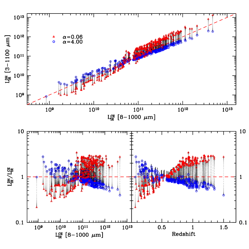
Figure 7.— Comparison of two independent derivations of the infrared luminosity $L_{IR}$ for sources in our sample. In the top panel, the best-fit $L_{IR}^{CE}$ for each source in our sample is compared to a range of $L_{IR}^{DH}$ computed for the full family of DH02 SEDs (black dots). Open symbols represent the limiting ‘hot’ ($\alpha=$0.06; red triangles) and ‘cold’ ($\alpha=$4.00; blue circles) DH02 SEDs. The bottom panels are residual plots shown as functions of $L_{IR}^{CE}$ (lower-left) and redshift (lower-right). This figure shows that $L_{IR}^{CE}$, adopted as our best-fit bolometric luminosity is consistent with the range of $L_{IR}^{DH}$ that one obtains if no $L_{MIR}-L_{IR}$ correlation is assumed.

4. AGN Contamination

The conversions of both emission line and $L_{IR}$ luminosity to a star formation rate hinge on the assumption that the dominant ionization and heating source is radiation from massive young stars. AGN-dominated emission line and IR fluxes do not trace star formation and must therefore be removed from our sample. Various emission-line diagnostics such as [OIII]/$H\beta$ versus [NII]/$H\alpha$ and [OIII]/$H\beta$ versus [SII]/$H\alpha$ effectively separate populations with different ionization sources (Osterbrock, 1989). In cases with more limited spectral coverage, individual line ratios such as [NeIII]/[OII] have also been successfully utilized (Kobulnicky & Kewley, 2004). We do not employ these line diagnostics, due to the non-uniform rest-frame spectral coverage of our sample. Instead, we rely on an IRAC color selection and the visual identification of optical spectral features to identify and remove AGN candidates from our sample.

We first flag sources with obvious AGN signatures such as broadened Balmer and/or [OII] lines or strong NeIII or NeV emission. Next, we combine our sample with IRAC photometry of the FLS (Lacy et al., 2005) to implement a 4-band IRAC color selection. It has been shown that AGN can be identified in the MIR, based on their strong continuum flux (Laurent et al., 2000; Lacy et al., 2004; Stern et al., 2005). Lacy et al. (2004) use 4-band Spitzer IRAC photometry (3.6, 4.5, 5.8 & 8.0µm) to identify a distinct region in color-color space where quasars and AGN are likely to be found. In Figure 8a, we reproduce the IRAC color-color plot from Lacy et al. (2004) (Figure 1) for the entire FLS main field. The dashed line shows the region expected to be occupied by AGN. In Figure 8b we show the same plot for our current sample. The FLS depth of the IRAC channels 3 & 4 is slightly shallower than that of channels 1 & 2, and only 2/3 of our sample have clean photometry in all four IRAC bands (open circles); for the remaining 1/3 of the sample, limiting flux ratios are shown (open triangles). Based on the IRAC color selection, $9\%$ of each of these subsamples fall in the AGN-candidate region. Visual re-inspection of the 16 IRAC-selected candidates, reveals that $63\%$ exhibit some AGN signature in their spectra (6 strong; 4 moderate). The remaining sources show no obvious indicator; however, an AGN contribution cannot be ruled out, given our limited spectral coverage. We remove all 16 candidates from the final sample. Investigation of the spectroscopically selected candidates shows that 5 of 9 sources (55%) with strong AGN spectral signatures are also IRAC-selected AGN. Ultimately, we find that neither the spectroscopic nor IRAC color selection provides a complete census of all AGN, so we take the conservative approach of combining the two methods to clean our sample. The impact of this AGN removal is best illustrated in the comparison of the two different SFR diagnostics (Fig. 9), discussed in the next section.

Figure 8.— IRAC 4-channel color-color plots used to identify AGN candidates. Panel (a) illustrates how the AGN candidate region of color-color space is defined by Lacy et al. (2004). All sources with clean 4-color photometry from the full 4 sq. deg FLS main field are plotted; the region in which quasars and AGN are expected to be found is marked by a dashed line (cf. Sajina, Lacy, & Scott, 2005, for details). Panel (b) shows our sample with the same AGN region marked. The majority of the sample ($\approx\!2/3$) has clean photometry in all four IRAC bands (open circles). The remaining sources ($\approx\!1/3$) have at least two measured fluxes and therefore at least one limiting color (open triangles). Sources that fall in the dashed region of this color-color diagram are flagged as AGN candidates and are removed from our final sample.

5. Optical vs. IR SFR comparison

Next, we compare the two independently derived SFR diagnostics $SFR_{opt}$ and $SFR_{IR}$ described in §3 for the full AGN-cleaned sample. In Figure 9, we show the reddening-uncorrected, emission line-derived $SFR_{opt}$ versus the IR luminosity-derived $SFR_{IR}$, before and after AGN removal. The sample plotted in Figure 9 (left) includes the 274 sources with well determined spectroscopic redshifts, emission line and 24µm  fluxes. AGN candidates are marked based on their spectral (squares) or IRAC color identification (circles) (as discussed in §4). In Figure 9 (right) only the final 241 source AGN-removed sample is shown. Though the distribution of the AGN candidates are not localized to a single region of the plot, sources with the most extreme SFR discrepancies tend to be AGN. This illustrates the potential for these sources to be misidentified as heavily obscured galaxies. The inclusion of this population would bias the sample to appear overly obscured. The fact that AGN candidates are found throughout the SFR vs SFR plot is not unexpected since the emission line luminosity and IR luminosity are loosely correlated in AGN.

Figure 9.— Comparison of $SFR_{opt}$ and $SFR_{IR}$ before (left) and after (right) AGN removal. In the left panel a sample of 274 sources with well-determined emission lines and IR luminosity are plotted as crosses. The 33 AGN candidates identified by their spectral features (squares) and IRAC colors (circles) are marked. In the right panel, the final 241 source sample after AGN removal is shown. No extinction correction has been applied to $SFR_{opt}$ in either panel. Representative error bars are shown in each panel. The $SFR_{opt}$ error bar is the mean $1\sigma$ uncertainty due to the error in line flux measurement. The $SFR_{IR}$ error bar is the mean of the bolometric correction uncertainty, as discussed in §3.2.1. The comparison of these samples illustrates 1) the importance of limiting the AGN contamination and 2) that without any reddening correction, $SFR_{opt}$ severely underestimates the true star formation rate, especially for our most IR luminous sources.

In Figure 9 (right) the uncorrected $SFR_{opt}$ is systematically lower than $SFR_{IR}$ . Over the $L_{IR}$ range of our sample, the offset spans 2 orders of magnitude and illustrates the importance of properly accounting for the optical extinction. In this section we explore a range of different extinction corrections to reconcile the two SFRs. In Figure 10, the ratio of the two diagnostics, $SFR_{opt}$/$SFR_{IR}$ is plotted to better illustrate the systematic difference between them. It is evident from Figure 10a, in which no reddening correction has been applied that $SFR_{opt}$ underestimates the true SFR by anywhere from $0-2.5$ dex. In the remaining panels, we investigate the applicability of various fixed extinction corrections. In Figure 10(b), an extinction of $A_{v}=1.0$, representative of normal spiral galaxies is assumed. This is a significant improvement over the uncorrected $SFR_{opt}$, especially at low IR luminosity, typical of normal late-type galaxies. Beyond $L_{IR}>10^{10}L_{\odot}$, however, the two $SFRs$ diverge, indicating that this standard correction underestimates the attenuation in starburst and brighter galaxies. In Figures 10c & d, we adopt more extreme corrections of $A_{v}=2.0$ mag and $A_{v}=3.0$ mag and find that neither provides a good solution over the full range in $L_{IR}$. The Calzetti et al. (2000) reddening curve is adopted for each of these corrections. We conclude that a constant $A_{v}$ correction is insufficient for reconciling $SFR_{opt}$ and $SFR_{IR}$. In the following sections, we take two independent approaches to characterize the optical extinction of galaxies of our sample. In the first, we use Balmer decrement and other emission line ratios to compute extinction, $A_{v}^{em}$. In the second, we adopt $SFR_{IR}$ as a proxy for the true total star formation rate and compute $A_{v}^{IR}$ based on the difference between $SFR_{opt}$ and $SFR_{IR}$.

Figure 10.— $SFR_{opt}/SFR_{IR}$ vs. $SFR_{IR}$ and $L_{IR}$ for the final AGN-cleaned sample, shown for a range of constant extinction corrections. In panel (a) no correction for any optical extinction is made. In panel (b) a uniform standard correction of $A_{v}=1.0$ mag, typical of normal spiral galaxies, is applied to $SFR_{opt}$. In panels (c & d) more extreme constant extinction corrections, $A_{v}=2.0$ mag and $A_{v}=3.0$ mag are adopted. Representative error bars are shown in each panel. The $SFR_{opt}/SFR_{IR}$ error bar includes only the mean $1\sigma$ uncertainty due to the error in line flux measurement, it does not include any uncertainty in $SFR_{IR}$. The $SFR_{IR}$ error bar is the mean of the bolometric correction uncertainty, as discussed in §3.2.1. With no extinction correction, $SFR_{opt}$ underestimates the true star formation rate by as much as 2.5 dex for our most IR luminous sources. Uniform extinction corrections do not adequately represent our sample of normal, starburst and LIRG galaxies.

5.1. Optical Extinction Correction I: Balmer Decrement

A standard method for measuring the internal extinction of an individual galaxy is through the comparison of observed to predicted Balmer line ratios. We adopt this approach for the subset of our sample with multiple measured Balmer lines. The color excess $E(B-V)_{gas}$ of a source is computed by comparing the observed Balmer line ratios $(F_{o}^{H\alpha}/F_{o}^{H\beta})$, $(F_{o}^{H\delta}/F_{o}^{H\beta})$ and $(F_{o}^{H\gamma}/F_{o}^{H\beta})$ with their intrinsic unobscured ratios:

$$E(B-V)_{gas}=\frac{2.5}{[k(\lambda_{1})-k(\lambda_{2})]}\log\frac{(F_{i}^{\lambda_{1}}/F_{i}^{\lambda_{2}})}{(F_{o}^{\lambda_{1}}/F_{o}^{\lambda_{2}})}$$ (11)

where ($F_{i}^{\lambda_{1}}/F_{i}^{\lambda_{2}}$) are the intrinsic unobscured line ratios based on case-B recombination and $T=10,000$ K (Osterbrock, 1989). The obscuration or reddening curve ($k(\lambda)$) has been derived by Calzetti et al. (2000) for starburst galaxies:

$$k(\lambda)=\cases{2.659(-1.857+1.040/\lambda)+R_{v}\cr\qquad(0.63\micron\leq\lambda\leq 2.20\micron)\cr\cr 2.659(-2.156+1.509/\lambda\cr-0.198/\lambda^{2}+0.011/\lambda^{3})+R_{v}\cr\qquad(0.12\micron\leq\lambda\leq 0.63\micron)}$$ (12)

It should be noted that although there are significant large-scale differences between the various starburst, Milky Way, LMC and SMC reddening curves, over the rest-frame spectral region covered by the emission lines of interest (3700Å$\lesssim\lambda\lesssim$6600Å), the differences are minor (Calzetti, 2001, and references therein). The color excess is converted into a wavelength dependent extinction based on:

$$A(\lambda)=E(B-V)_{gas}k(\lambda)$$ (13)

where A($\lambda$) is the mean emission line derived extinction in units of magnitudes at the wavelength $\lambda$. This should be distinguished from $A_{s}(\lambda)$, the extinction as measured from the stellar continuum. As has been shown by Calzetti (2001) these differ by a factor of 0.44 in typical local starbursts.

Figure 11.— $SFR_{opt}/SFR_{IR}$ versus $SFR_{IR}$ and $L_{IR}$ before and after application of emission line ratio-derived reddening corrections, $A_{v}^{em}$. A sample of 24 sources is shown (crosses) before (left) and after (right) the application of $A_{v}^{em}$. For reference, the full sample is also plotted (small dots). The $SFR_{IR}$ error bars represent the full range of the bolometric correction uncertainty, as discussed in §3.2.2. The $SFR_{opt}/SFR_{IR}$ error bars show the $1\sigma$ uncertainty due to the error in line flux measurement, excluding any contribution from $SFR_{IR}$. In panel b, individual y-error bars also include the uncertainty in $A_{v}^{em}$. Application of $A_{v}^{em}$ results in a reasonable ensemble-averaged SFR, as evidenced by the improvement of $\langle log(SFR_{opt}/SFR_{IR})\rangle$ from -0.98 to -0.07. However, the significant increase in scatter suggests that our emission line ratios do not provide optimal corrections for individual sources.

In addition to using the Balmer decrement, we explore the possibility of using the [OII]/$H\beta$ line ratio to compute $A_{v}^{em}$. Though this ratio is less certain than that of the Balmer lines, we adopt an empirical value for the intrinsic [OII]/$H\beta$ line ratio based on the locally measured reddening-corrected line fluxes. Using the NFGS, Kewley, Geller, & Jansen (2004) measure a mean extinction-corrected [OII]/$H\alpha$ ratio of 1.2, which translates to an [OII]/$H\beta$ line ratio of:

$$F_{i}^{[OII]}/F_{i}^{H\beta} =3.44$$

From our full sample, individual reddening corrections, $A_{v}^{em}$, are computed for 24 sources that have multiple strong Balmer and/or [OII] emission lines. Line fluxes and $SFR_{opt}$ are then reddening-corrected on a source-by-source basis. In Figure 11, $SFR_{opt}/SFR_{IR}$ vs. $SFR_{IR}$ for this sample (crosses) is shown before (left) and after (right) application of this correction. There is a significant increase in the scatter of the distribution after application of the extinction correction. This illustrates that due to the enormous uncertainties associated with $A_{v}^{em}$, source-by-source corrections are futile. Despite the increased scatter, it is noteworthy that $SFR_{opt}$ becomes consistent on average with $SFR_{IR}$, with the mean offset reduced from -0.98 dex to -0.07 dex. This indicates that in the absence of other extinction indicators, with a large enough sample and careful stellar absorption measurements, Balmer decrement and [OII]/$H\beta$ emission line ratios can provide a reasonable first order $\langle A_{v}^{em}\rangle$ correction for the luminosity range of this sample. The median emission line derived extinction of this subsample is $\tilde{A}_{v}^{em}=1.5\pm 1.1$ mag with $\langle SFR_{IR}\rangle=23\pm 8~{}M_{\odot}yr^{-1}$. Due to the relatively small size and limited $L_{IR}$ coverage of this subsample, along with the large uncertainties, we are not able to derive an $L_{IR}$-dependent extinction correction. Instead, in the next section we adopt $SFR_{IR}$ as a ‘true’ SFR and compare it to the extinction-uncorrected $SFR_{opt}$ to derive $A_{v}^{IR}$ for the full sample.

5.2. Optical Extinction Correction II: IR vs Optical SFRs

5.2.1 Computing $A_{v}^{IR}$

In this section, we take an alternative approach of adopting $SFR_{IR}$ as a proxy for the true SFR to determine the extinction correction of our sample. Specifically, the ratio $SFR_{IR}$ over the uncorrected $SFR_{opt}$ is used to compute the attenuation of the given emission line:

$$A(\lambda)=-2.5*\log(SFR_{opt}/SFR_{IR})$$ (14)

where $\lambda$ is the wavelength of the emission line used to compute $SFR_{opt}$. $A(\lambda)$ is converted to a standard visual extinction, $A_{v}$ by:

$$A_{v}=\frac{A(\lambda)}{k(\lambda)}k_{v}$$ (15)

Extinction derived in this manner may have a large uncertainty for individual sources, but this approach should produce a reasonable ensemble average. In Figure 12, $A_{v}^{IR}$ versus $SFR_{IR}$ and $L_{IR}$ is shown for our full sample. Despite the large scatter in the distribution, a clear trend of increasing $A_{v}^{IR}$ as a function of $SFR_{IR}$ is evident. The best-fit line to this distribution is:

$$A_{v}^{IR}=0.75(\log(SFR_{IR}))+1.05$$ (16)

which in terms of $L_{IR}$ is:

$$A_{v}^{IR}=0.75*\log(L_{IR}/L_{\odot})-6.35$$ (17)

This fit is limited to starburst and brighter systems ($L_{IR}>10^{10}L_{\odot}$; orange solid line), where $SFR_{IR}$ is a good representation of the total SFR. It is extrapolated to lower luminosities ($L_{IR}<10^{10}L_{\odot}$; orange dotted line). Inclusion of the full sample has only a minor effect, slightly steepening the fit. The mean $A_{v}^{IR}$ values (black dots) of sources binned in $log(SFR_{IR})$ are overlaid along with error bars that show their $1\sigma$ dispersion.

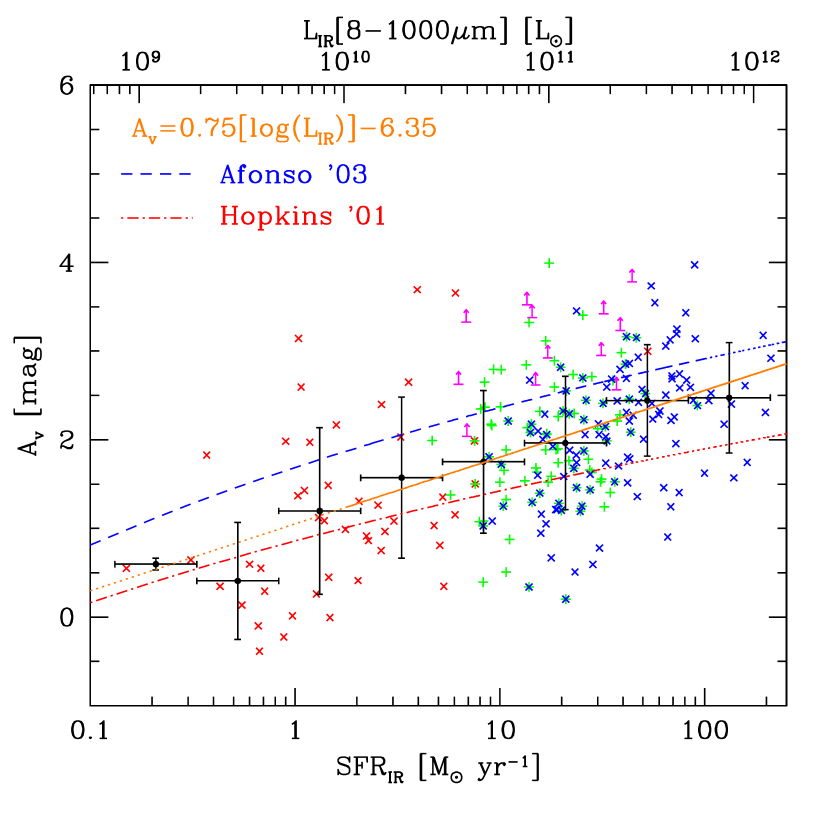
Figure 12.— Optical extinction $A_{v}^{IR}$ vs. $L_{IR}$ for the complete galaxy sample. $A_{v}^{IR}$ is derived from the ratio of $SFR_{opt}/SFR_{IR}$, where $SFR_{IR}$ is adopted as a proxy for the true SFR, and plotted as a function of IR luminosity (crosses & pluses). Sources with measured $H\alpha$, $H\beta$ & [OII] line fluxes are shown as red, green and blue points, respectively. Those with only emission line flux limits are shown as magenta arrows. Mean $A_{v}^{IR}$ values (solid circles), binned in $log(SFR_{IR})$ are plotted along with their $1\sigma$ uncertainties. The best-fit line $A_{v}^{IR}=0.75*log(L_{IR}/L_{\odot})-6.35$ mag is computed and overlaid as a solid orange line and compared to those derived by Hopkins et al. (2001) (dot-dashed red) and Afonso et al. (2003) (dashed blue). Extrapolations beyond the dataset luminosity limits are indicated by dotted lines. The mean measured $A_{v}^{IR}$ function of our sample is intermediate between those of H01 & A03, with evidence for a stronger $L_{IR}$ dependence.

5.2.2 Comparison to Local Samples

We make a direct comparison of our $A_{v}^{IR}$ function to those of local optical/UV Hopkins et al. (2001) and radio-selected samples of Afonso et al. (2003) (hereafter H01 & A03). We transform their E(B-V) color excess to $A_{v}$ based on $R_{v}=3.1$ and plot them as red dot-dashed & blue dashed curves, with dotted segments representing extrapolations beyond their datasets. For a given SFR, the mean $A_{v}^{IR}$ of our sample is intermediate between those of H01 and A03. The trend in the extinction as a function of $L_{IR}$ is also slightly steeper than the previous relationships. To interpret these differences requires a closer examination of the various sample selections.

The H01 SFR dependent extinction relationship is based on small ($N\!\approx\!60$) local UV+optical selected samples (cf. Sullivan et al. (2001)), whereas that of A03 is derived from a comparably sized radio-selected sample that extends to slightly higher redshift $\langle z\rangle\approx\!0.25$ and is more actively starforming. The difference in the mean $A_{v}$ between the two samples is attributed to the fact that optical/UV selected samples are biased against heavily obscured galaxies. Our initial spectroscopic sample being NIR-selected ($2.2\micron$), we expect our sample to be significantly less affected by obscuration effects than that of a UV/optical sample. It is therefore not surprising that our mean $A_{v}^{IR}$ is higher than that of H01.

The discrepancy between our sample and that of A03 is more difficult to understand since both radio and NIR/MIR selections should be relatively robust against obscuration biases. It is suggestive of a selection bias in one or both samples. Reliance on optical spectroscopy may be one potential culprit. It is possible that the dustiest systems are so heavily obscured that either their redshifts are indeterminable or their emission lines are completely attenuated. We can place some constraints on the sizes of these two populations in our sample. Our spectroscopic redshift efficiency of $92\pm 5\%$ places an 8% limit on the first. This is a conservative estimate since some fraction of the 8% are certainly due to our spectroscopic redshift sensitivity function dropping off beyond $z\!\approx\!1.3$. Regarding the second population, 12 sources in our sample ($<4\%$) with identified redshifts, have no measured emission line fluxes and therefore only lower limits on the derived attenuation. These are shown as arrows in Figures 9 & 12 and included in our $A_{v}^{IR}(L_{IR})$ estimate. Deeper optical spectroscopy may reveal these to be even more heavily obscured systems. Based on these estimates, these two populations are likely to account for $\lesssim 10\%$ of the total population. It is worth noting that these biases are not unique to this study since most surveys rely on optical spectroscopy for redshift and/or emission line diagnostics.

One potential bias that may overestimate the mean optical attenuation is due to AGN contamination. Especially in the most luminous samples, the contribution from AGN becomes increasingly significant. Radio-selected, and to a lesser extent, MIR-selected samples will tend to have larger fractions of ‘active’ galaxies than comparable depth optical or NIR samples. As seen in Figure 9, if this population is not sufficiently screened, it can result in an overestimate of the sample $A_{v}$.

Figure 13.— $SFR_{opt}/SFR_{IR}$ vs. $SFR_{IR}$ and $L_{IR}$ of the final AGN-cleaned sample, with various luminosity dependent extinction corrections. In panel (a) no correction for any optical extinction is made. In panels (b & c) we adopted the $A_{v}$ functions derived by H01 and A03 respectively. In panel (d) we adopt our best-fit $A_{v}^{IR}$ extinction function based on our sample. Representative error bars are the same as in Figure 10. We see that the corrections of H01 and A03 appear to under/over-estimate the mean extinction of our sample. The scatter of the corrected sample in panel (d) is 0.3 dex.

Finally, our $A_{v}^{IR}$ values appear to be consistent with those derived from an SDSS sample of starforming galaxies (Hopkins et al., 2003). Though no direct comparison is shown here, inspection of their Figure 8 shows that the mean $A_{v}$ of their sample is intermediate between that of H01 and A03, consistent with the correction derived here over a comparable range of SFR.

5.2.3 Disentangling the $L_{IR}$ vs. Redshift Dependence

As seen in Figure 6, our sample spans a broad range in both IR luminosity and redshift; and as a consequence of our 24µm  flux limit it exhibits a strong $L_{IR}$-redshift correlation. So far, we have been assuming that for a fixed $L_{IR}$, $A_{V}$ is largely redshift independent. Given the potential degeneracy between redshift and IR luminosity dependencies, the validity of this assumption merits investigation.

Though our sample is not ideally suited for a thorough study of this issue, we can place some limits on the redshift dependence by isolating subsets of our data restricted in IR luminosity and redshift. In Figure 14, we take a look at two such slices in $L_{IR}$ and redshift. The first is restricted to $2\times 10^{11}<L_{IR}/L_{\odot}<1\times 10^{12}$, and the second to $0.7<z<1.0$. In the lower panels, plots of $A_{V}$ vs. redshift and $A_{V}$ vs. $L_{IR}$ for the respective subsets reveal that a) for a sample with a narrow range of $L_{IR}$, there is no strong trend in $A_{V}$ with redshift; and b) over a relatively narrow redshift slice centered at $z=0.85$, $A_{V}$ shows a clear correlation with $L_{IR}$. Though our sample does not allow us to investigate trends over the entire redshift or $L_{IR}$ range of our sample, these two slices suggest that to first order the dependence on redshift is small compared to that on $L_{IR}$.

Figure 14.— A comparison of the $A_{V}^{IR}$ dependence on IR luminosity and redshift for two subsets of our final sample. In the $L_{IR}$ versus redshift plot (top), two regions limited in $L_{IR}$ ($2\times 10^{11}<L_{IR}<1\times 10^{12}$) and redshift ($0.7<z<1.0$) are identified with dashed & dotted lines and marked A & B, respectively. The lower panels show $A_{V}^{IR}$ vs. redshift for 122 galaxies from region A (lower-left) and $A_{V}^{IR}$ vs. $L_{IR}$ for 115 galaxies from region B (lower-right). The lower-left panel reveals that for a fixed $L_{IR}$, $A_{V}$ exhibits almost no redshift dependence. By contrast, the lower-right panel shows that even over a narrow redshift range, $A_{V}$ has a clear $L_{IR}$ dependence.

6. Summary

We have combined MIR (24µm) photometry with high-resolution, optical spectroscopy for a large ($N\,=\,241$), $Ks+MIPS\,24\micron$-selected ($K_{s}\,<\,20.2$ mag; $f24\,>\,80\mu Jy$) galaxy sample. AGN are removed by implementing both spectroscopic and MIR color selections. This dataset is used to measure the instantaneous star formation rate and the mean attenuation of normal through IR luminous galaxies ($10^{9}<L_{IR}<10^{12.5}L_{\odot}$; $\langle L_{IR}\rangle=1.8\times 10^{11}L_{\odot}$; $\langle SFR\rangle=31~{}M_{\odot}yr^{-1}$ ) out to a redshift of $z<1.5$ ($\langle z\rangle=0.77$). We compare two independent approaches of computing the star formation rate. The first is based on the IR luminosity, $SFR_{IR}$, and the second is based on optical Balmer and [OII] emission line fluxes, $SFR_{opt}$.

Comparison of the two SFR diagnostics reveal that with no correction for extinction, the optical SFR systematically underestimates the IR SFR by as much as 2.5 dex. This discrepancy has a clear IR luminosity dependence that cannot by reconciled with a constant $A_{v}$ extinction correction. We take two independent approaches to investigate the dust attenuation of our sample.

First, we compute Balmer decrement and emission line ratio derived optical extinction $A_{v}^{em}$ on a source-by-source basis for a subset of our sample. We find that after correction, despite a large scatter in the distribution, the ensemble averaged $SFR_{opt}$ is consistent with $SFR_{IR}$. The large errors associated with the derived $A_{v}^{em}$, however, illustrate that even with the stellar continuum properly measured, the high-order Balmer line ratios, such as $H\beta/H\gamma$ and $H\beta/H\delta$, as well as [OII]/$H\beta$ have only a limited usefulness for extinction corrections of individual galaxies at high redshift. This is due to: a) the relative weakness of these high order emission lines; and b) the limited leverage afforded by the narrow separation of these lines, in comparison to the conventionally adopted $H\alpha$/$H\beta$ Balmer decrement.

As an alternative measure of the optical attenuation, we use $SFR_{opt}/SFR_{IR}$, to derive an IR-luminosity dependent extinction function, $A_{v}^{IR}=0.75*log(L_{IR}/L_{\odot})-6.35$ mag. In comparing this relationship with local optical/UV and radio-selected samples, we find that our $A_{v}^{IR}$ function is intermediate between those of Hopkins et al. (2001), Sullivan et al. (2001) and Afonso et al. (2003) but with a slightly steeper slope. Though it is difficult to reconcile these results without a directly overlapping sample, we highlight some of the key differences that may contribute to the discrepancy. Afonso et al. (2003) suggests that the difference between their results is due to selection bias against highly obscured objects in the original Hopkins et al. (2001) sample. Our sample should be relatively free of this selection bias and therefore comparable to that of Afonso et al. (2003). The fact that they are not is a bit surprising, but may suggest that one or both of these samples is still suffering from an additional bias. One possibility is that we may be excluding the most highly obscured sources due to our spectroscopic sensitivities. This is not likely to have a dominant effect given the high $92\%$ spectroscopic redshift efficiency of our sample and the fact that all spectroscopic samples are affected by this bias. Another possibility is that the Afonso et al. (2003) sample, due to its radio-selected nature may contain a larger fraction of galaxies with AGN that may be inflating their mean $A_{v}$. The inclusion of even non-dominant AGN may have a similar effect on the measured ensemble extinction as that of a heavily dust-obscured population.

We do not attempt to quantify the $A_{V}$ evolution over our full redshift range. However, based on subsamples restricted to narrow redshift and $L_{IR}$ ranges, we find no evidence for significant $A_{V}$ evolution.

The scatter in $SFR_{opt}/SFR_{IR}$ after application of our best-fit attenuation correction, is larger than expected from either the line flux errors or the reasonable estimates of the IR bolometric correction uncertainty. The impact of adopting a mean metallicity correction ($\lesssim 0.1$ dex) also cannot account for this scatter. This indicates that these diagnostics are not providing consistent tracers of the current SFR, possibly due to differences in their dependence on dust geometry and/or SFR timescale.

7. Acknowledgements

We thank the anonymous referee for insightful comments that have significantly improved this paper. We would also like to thank Carol Lonsdale, Robert Kennicutt and Rolf Jansen for early discussions that helped shape this project. We thank all of our colleagues associated with the Spitzer mission, which has been carried out at the Jet Propulsion Laboratory, operated by California Institute of Technology, under NASA contract 1407. We are indebted to Grant Hill, Greg Wirth and the rest of the Keck observatory staff for their phenomenal observation support. The analysis pipeline used to reduce the DEIMOS data was developed by the DEEP2 group at UC Berkeley with support from NSF grant AST-0071048. Finally, we wish to recognize and acknowledge the significant cultural role and reverence that the summit of Mauna Kea has within the indigenous Hawaiian community. We are grateful for the opportunity to conduct observations from this mountain.

References

- Adelberger & Steidel (2000) Adelberger, K. L. & Steidel, C. C. 2000, ApJ, 544, 218
- Afonso et al. (2003) Afonso, J., Hopkins, A., Mobasher, B., & Almeida, C. 2003, ApJ, 597, 269
- Bell (2002) Bell, E. F. 2002, ApJ, 577, 150
- Bell (2003) —. 2003, ApJ, 586, 794
- Bell et al. (2002) Bell, E. F., Gordon, K. D., Kennicutt, R. C., & Zaritsky, D. 2002, ApJ, 565, 994
- Bell & Kennicutt (2001) Bell, E. F. & Kennicutt, R. C. 2001, ApJ, 548, 681
- Blanton et al. (2003) Blanton, M. R., et al. 2003, AJ, 125, 2348
- Buat et al. (2002) Buat, V., Boselli, A., Gavazzi, G., & Bonfanti, C. 2002, A&A, 383, 801
- Calzetti (2001) Calzetti, D. 2001, PASP, 113, 1449
- Calzetti et al. (2000) Calzetti, D., Armus, L., Bohlin, R. C., Kinney, A. L., Koornneef, J., & Storchi-Bergmann, T. 2000, ApJ, 533, 682
- Calzetti et al. (1994) Calzetti, D., Kinney, A. L., & Storchi-Bergmann, T. 1994, ApJ, 429, 582
- Cardiel et al. (2003) Cardiel, N., Elbaz, D., Schiavon, R. P., Willmer, C. N. A., Koo, D. C., Phillips, A. C., & Gallego, J. 2003, ApJ, 584, 76
- Chary & Elbaz (2001) Chary, R. & Elbaz, D. 2001, ApJ, 556, 562
- Condon (1992) Condon, J. J. 1992, ARA&A, 30, 575
- Cram et al. (1998) Cram, L., Hopkins, A., Mobasher, B., & Rowan-Robinson, M. 1998, ApJ, 507, 155
- Dale & Helou (2002) Dale, D. A. & Helou, G. 2002, ApJ, 576, 159
- Desert et al. (1990) Desert, F.-X., Boulanger, F., & Puget, J. L. 1990, A&A, 237, 215
- Diolaiti et al. (2000) Diolaiti, E., Bendinelli, O., Bonaccini, D., Close, L., Currie, D., & Parmeggiani, G. 2000, A&AS, 147, 335
- Dopita et al. (2002) Dopita, M. A., Pereira, M., Kewley, L. J., & Capaccioli, M. 2002, ApJS, 143, 47
- Elbaz et al. (2002) Elbaz, D., Cesarsky, C. J., Chanial, P., Aussel, H., Franceschini, A., Fadda, D., & Chary, R. R. 2002, A&A, 384, 848
- Erb et al. (2003) Erb, D. K., Shapley, A. E., Steidel, C. C., Pettini, M., Adelberger, K. L., Hunt, M. P., Moorwood, A. F. M., & Cuby, J. 2003, ApJ, 591, 101
- Faber et al. (2003) Faber, S. M., et al. 2003, in Instrument Design and Performance for Optical/Infrared Ground-based Telescopes. Edited by Iye, Masanori; Moorwood, Alan F. M. Proceedings of the SPIE, Volume 4841, pp. 1657-1669 (2003)., 1657–1669
- Fadda et al. (2004) Fadda, D., Jannuzi, B. T., Ford, A., & Storrie-Lombardi, L. J. 2004, AJ, 128, 1
- Fazio et al. (2004) Fazio, G. G., et al. 2004, ApJS, 154, 10
- Flores et al. (2004) Flores, H., Hammer, F., Elbaz, D., Cesarsky, C. J., Liang, Y. C., Fadda, D., & Gruel, N. 2004, A&A, 415, 885
- Gallagher et al. (1989) Gallagher, J. S., Hunter, D. A., & Bushouse, H. 1989, AJ, 97, 700
- Ghosh & White (2001) Ghosh, P. & White, N. E. 2001, ApJ, 559, L97
- Glazebrook et al. (1999) Glazebrook, K., Blake, C., Economou, F., Lilly, S., & Colless, M. 1999, MNRAS, 306, 843
- Goldader et al. (2002) Goldader, J. D., Meurer, G., Heckman, T. M., Seibert, M., Sanders, D. B., Calzetti, D., & Steidel, C. C. 2002, ApJ, 568, 651
- Helou (2000) Helou, G. 2000, in Infrared Space Astronomy, Today and Tomorrow, 337–+
- Helou & Bicay (1993) Helou, G. & Bicay, M. D. 1993, ApJ, 415, 93
- Helou et al. (1985) Helou, G., Soifer, B. T., & Rowan-Robinson, M. 1985, ApJ, 298, L7
- Hippelein et al. (2003) Hippelein, H., et al. 2003, A&A, 402, 65
- Hogg et al. (1998) Hogg, D. W., Cohen, J. G., Blandford, R., & Pahre, M. A. 1998, ApJ, 504, 622
- Hopkins et al. (2001) Hopkins, A. M., Connolly, A. J., Haarsma, D. B., & Cram, L. E. 2001, AJ, 122, 288
- Hopkins et al. (2003) Hopkins, A. M., et al. 2003, ApJ, 599, 971
- Kennicutt (1992) Kennicutt, R. C. 1992, ApJS, 79, 255
- Kennicutt (1998) —. 1998, ARA&A, 36, 189
- Kewley et al. (2004) Kewley, L. J., Geller, M. J., & Jansen, R. A. 2004, AJ, 127, 2002
- Kewley et al. (2002) Kewley, L. J., Geller, M. J., Jansen, R. A., & Dopita, M. A. 2002, AJ, 124, 3135
- Kobulnicky & Kewley (2004) Kobulnicky, H. A. & Kewley, L. J. 2004, ApJ, 617, 240
- Lacy et al. (2004) Lacy, M., et al. 2004, ApJS, 154, 166
- Lacy et al. (2005) Lacy, M., et al. 2005, ApJ, Submitted
- Laurent et al. (2000) Laurent, O., Mirabel, I. F., Charmandaris, V., Gallais, P., Madden, S. C., Sauvage, M., Vigroux, L., & Cesarsky, C. 2000, A&A, 359, 887
- Lonsdale-Persson & Helou (1987) Lonsdale-Persson, C. J. & Helou, G. 1987, ApJ, 314, 513
- Madau et al. (1996) Madau, P., Ferguson, H. C., Dickinson, M. E., Giavalisco, M., Steidel, C. C., & Fruchter, A. 1996, MNRAS, 283, 1388
- Marleau et al. (2004) Marleau, F. R., et al. 2004, ApJS, 154, 66
- McGaugh (1991) McGaugh, S. S. 1991, ApJ, 380, 140
- Osterbrock (1989) Osterbrock, D. E. 1989, Astrophysics of gaseous nebulae and active galactic nuclei (Research supported by the University of California, John Simon Guggenheim Memorial Foundation, University of Minnesota, et al. Mill Valley, CA, University Science Books, 1989, 422 p.)
- Rieke et al. (2004) Rieke, G. H., et al. 2004, ApJS, 154, 25
- Rigopoulou et al. (2000) Rigopoulou, D., et al. 2000, ApJ, 537, L85
- Sajina et al. (2005) Sajina, A., Lacy, M., & Scott, D. 2005, ApJ, 621, 256
- Sanders & Mirabel (1996) Sanders, D. B. & Mirabel, I. F. 1996, ARA&A, 34, 749
- Silva et al. (1998) Silva, L., Granato, G. L., Bressan, A., & Danese, L. 1998, ApJ, 509, 103
- Stern et al. (2005) Stern, D., et al. 2005, ApJ, 631, 163
- Sullivan et al. (2001) Sullivan, M., Mobasher, B., Chan, B., Cram, L., Ellis, R., Treyer, M., & Hopkins, A. 2001, ApJ, 558, 72
- Sullivan et al. (2004) Sullivan, M., Treyer, M. A., Ellis, R. S., & Mobasher, B. 2004, MNRAS, 350, 21
- Takeuchi et al. (2005) Takeuchi, T. T., Buat, V., Iglesias-Páramo, J., Boselli, A., & Burgarella, D. 2005, A&A, 432, 423
- Tresse & Maddox (1998) Tresse, L. & Maddox, S. J. 1998, ApJ, 495, 691
- Yan et al. (1999) Yan, L., McCarthy, P. J., Freudling, W., Teplitz, H. I., Malumuth, E. M., Weymann, R. J., & Malkan, M. A. 1999, ApJ, 519, L47