Low Mach Number Modeling of Type Ia Supernovae

Abstract

We introduce a low Mach number equation set for the large-scale numerical simulation of carbon-oxygen white dwarfs experiencing a thermonuclear deflagration. Since most of the interesting physics in a Type Ia supernova transpires at Mach numbers from 0.01 to 0.1, such an approach enables both a considerable increase in accuracy and savings in computer time compared with frequently used compressible codes. Our equation set is derived from the fully compressible equations using low Mach number asymptotics, but without any restriction on the size of perturbations in density or temperature. Comparisons with simulations that use the fully compressible equations validate the low Mach number model in regimes where both are applicable. Comparisons to simulations based on the more traditional anelastic approximation also demonstrate the agreement of these models in the regime for which the anelastic approximation is valid. For low Mach number flows with potentially finite amplitude variations in density and temperature, the low Mach number model overcomes the limitations of each of the more traditional models and can serve as the basis for an accurate and efficient simulation tool.

1 Introduction

A broad range of interesting phenomena in science and engineering occur in a low Mach number regime in which the fluid velocity is much less than the speed of sound. Several low Mach number schemes have been developed to exploit this separation of scales; these models capture the fluid dynamics of interest without the need to resolve acoustic wave propagation. Physically, one can think of the solution to a low Mach number model as supporting infinitely fast acoustic equilibration rather than finite-velocity acoustic wave propagation. Mathematically, this is manifest in the addition of a constraint on the velocity field to the system of evolution equations. This velocity constraint can be translated into an elliptic equation for pressure that expresses the equilibration process. Because explicit discretization schemes for the low Mach number system are limited by the fluid velocity and not by the sound speed, they often gain several orders of magnitude in computational efficiency over the traditional compressible approach.

The simplest low Mach number model is expressed by the incompressible Navier-Stokes equations for a constant density fluid. Generalizations that incorporate variations in density include the Boussinesq approximation (Boussinesq, 1903), which allows heating-induced buoyancy in a constant density background, and the anelastic atmospheric (Batchelor, 1953; Ogura & Phillips, 1962; Dutton & Fichtl, 1969; Gough, 1969; Lipps & Hemler, 1982, 1985; Lipps, 1990; Wilhelmson & Ogura, 1972) and stellar (Latour et al., 1976; Gilman & Glatzmaier, 1981; Glatzmaier, 1984) approximations that include the effect of large-scale background stratification in the fluid density and pressure but assume small thermodynamic perturbations from the background. Low Mach number models for chemical combustion (Rehm & Baum, 1978; Majda & Sethian, 1985; Day & Bell, 2000) and nuclear burning (Bell et al., 2004) incorporate large compressibility effects due to chemical/nuclear reactions and thermal processes with a spatially constant background pressure.

Low Mach number models to date have, with one exception, allowed either zero volumetric changes (incompressible Navier-Stokes, Boussinesq) or changes due only to local heating effects (low-speed combustion, nuclear burning), or to large-scale background stratification (anelastic). The only low Mach number model that incorporates both finite local expansion due to heating and volume changes due to background stratification is the pseudo-incompressible equation set for the terrestrial atmosphere, introduced by Durran (1989) and rigorously derived using low Mach number asymptotics by Botta et al. (1999). The formulation of the pseudo-incompressible constraint assumes the ideal gas equation of state, which results in a simplification of terms that does not hold for more general equations of state and non-trivial changes in composition.

Our anticipated application for this model is the convective, ignition, and early propagation phases of Type Ia supernovae, but the model should be applicable to many other problems, such as Type I X-ray bursts (see, e.g., recent work by Lin (2005) for an alternate form of the low Mach number approach for Type I X-ray bursts), classical novae, and ordinary convection in stars. Events such as Type Ia supernovae are characterized by a large range in length scales, from the $O(10^{-4})$ to $O(10^{1})$ cm scale of the flame to the $O(10^{8})$ cm scale of the white dwarf. The range in timescales is equally impressive, from the 100 years of convection that precedes ignition to the one second duration of the explosion. Presently, most large-scale calculations focus on the explosion itself, beginning with several seeded hot spots to begin the runaway. In the last minutes of the convective phase, velocities reach $\sim 1\%$ of the sound speed (Woosley, 2001; Woosley et al., 2004), with temperature fluctuations of at most 5% (Wunsch & Woosley, 2004). These speeds are too slow for compressible codes to accurately follow. For this reason, simulation of the convective and ignition phases has seen only limited numerical work, e.g. Höflich & Stein (2002). Recent analytic work (Woosley et al., 2004) suggests that full star simulations are needed to accurately capture the convective flows and yield the spatial, temporal, and size distribution of the hot spots that seed the explosion. Three-dimensional anelastic calculations (Kuhlen et al., 2005) have shown that a dipole velocity field dominates the convection.

The low Mach number model presented here, like the anelastic model, will be capable of the long time integration necessary to follow the convection. Unlike the anelastic model, however, the low Mach number approach continues to be valid as the variation in density and temperature increases in the flame bubbles that evolve in the early phases of the explosion. Following the evolution from the convection through the early phases of the explosion is the eventual target of our low Mach number methodology.

Although the derivation of the low Mach number equation set will be general, the example we will consider is a simplified problem without reactions or thermal conduction, and with a time-independent radially symmetric form of self-gravity. The focus of the examples is to demonstrate the ability of the low Mach number model to accurately represent the hydrodynamics. We will compare the simulations based on the low Mach number approach to simulations based on the fully compressible equation set, where applicable, and to the traditional anelastic approach, where it is applicable. We will show that the low Mach number algorithm works well for very low Mach number flows, with validation presented up to Mach numbers $\sim 0.2$.

In the next section we derive the low Mach number equations, and in Section 3 we discuss the numerical implementation. Section 4 contains numerical comparisons with compressible and anelastic simulations, and in the final section we discuss our conclusions and future work.

2 Low Mach Number Model

We begin with the fully compressible equations governing motion in the stellar environment as described, for example, in Bell et al. (2004)

$$\frac{\partial\rho}{\partial t}+\nabla\cdot(\rho U) = 0\enskip,$$ (1)

$$\frac{\partial\rho U}{\partial t}+\nabla\cdot(\rho UU)+\nabla p = -\rho g\mathbf{e}_{r}\enskip,$$ (2)

$$\frac{\partial\rho E}{\partial t}+\nabla\cdot(\rho UE+pU) = \nabla\cdot(\kappa\nabla T)-\rho g(U\cdot\mathbf{e}_{r})-\sum_{k}{\rho q_{k}\dot{\omega}_{k}}\enskip,$$ (3)

$$\frac{\partial\rho X_{k}}{\partial t}+\nabla\cdot(\rho UX_{k}) = \rho\dot{\omega}_{k}\enskip.$$ (4)

Here $\rho$, $U$, $T$, and $p$ are the density, velocity, temperature and pressure, respectively, and $E=e+U\cdot U/2$ is the total energy with $e$ representing the internal energy. In addition, $X_{k}$ is the abundance of the $k$th isotope, with associated production rate, $\dot{\omega}_{k}$, and energy release, $q_{k}$. Finally, $g(r)$ is the radially dependent gravitational acceleration (resulting from spherically symmetric self-gravity), $\mathbf{e}_{r}$ is the unit vector in the radial direction, and $\kappa$ is the thermal conductivity. The Reynolds number of flows in a typical white dwarf is sufficiently large that we neglect viscosity here, though viscous terms could easily be included in the model and the numerical methodology.

For the stellar conditions being considered the pressure contains contributions from ions, radiation, and electrons. Thus

$$p=p(\rho,T,X_{k})=p_{\mathrm{ion}}+p_{\mathrm{rad}}+p_{\mathrm{ele}}\enskip,$$ (5)

where

$$p_{\mathrm{ion}}=\frac{\rho k_{B}T}{\bar{A}m_{p}}\enskip,\enskip\enskip p_{\mathrm{rad}}=aT^{4}/3\enskip,$$

and $p_{\mathrm{ele}}$ is the contribution to the thermodynamic pressure due to fermions. In these expressions $m_{p}$ is the mass of the proton, $a$ is related to the Stefan-Boltzmann constant $\sigma=ac/4$, $c$ is the speed of light, $\bar{A}=\sum_{k}{X_{k}A_{k}}$, $A_{k}$ is the atomic number of the $k$th isotope, and $k_{B}$ is Boltzmann’s constant. The ionic component has the form associated with an ideal gas but the radiation and electron pressure components do not. We use a stellar equation of state as implemented in Timmes & Swesty (2000).

As a prelude to developing the low Mach number equations, we first rewrite the energy equation (Eq. [3]) in terms of the enthalpy, $h=e+p/\rho$,

$$\rho\frac{Dh}{Dt}-\frac{Dp}{Dt} = \nabla\cdot(\kappa\nabla T)-\sum_{k}\rho q_{k}\dot{\omega}_{k}=\rho H\enskip,$$ (6)

where we introduce $H$ to represent the enthalpy source terms.

Our goal in this section is to derive a model for low speed flows in a hydrostatically balanced, radially stratified, background that removes acoustic waves yet allows for the development of finite amplitude temperature and density variations. We thus posit the existence of a background state with pressure, density and temperature $p_{0}(r,t),\rho_{0}(r,t)$ and $T_{0}(r,t)$ satisfying both the equation of state and hydrostatic equilibrium. Because we will neglect reaction terms that could potentially alter the large-scale pressure distribution within the star, for the purposes of this paper we will neglect time variation of the background state, i.e., we will assume $\partial p_{0}/\partial t=\partial\rho_{0}/\partial t=\partial T_{0}/\partial t=0$.

In order to understand the behavior of the system, we examine the balance of terms as a function of Mach number, $M=U/c_{s}$ ($c_{s}$ is the speed of sound), which will be assumed to be small. We re-write the momentum equation in nondimensional coordinates, where the space and time coordinates as well as the density, velocity and pressure, are scaled by characteristic values $L_{\mathrm{ref}}$, $t_{\mathrm{ref}},$ $\rho_{\mathrm{ref}},p_{\mathrm{ref}},$ and $U_{\mathrm{ref}}$, respectively. For the problem scale of interest $U_{\mathrm{ref}}$ is a typical advective velocity, $L_{\mathrm{ref}}$ a typical length scale, $t_{\mathrm{ref}}=L_{\mathrm{ref}}/U_{\mathrm{ref}}$, and $p_{\mathrm{ref}}=\rho_{\mathrm{ref}}\;c_{s_{\mathrm{ref}}}^{2}$, where $c_{s_{\mathrm{ref}}}$ is a characteristic value of $c_{s}$. We define a scaling for $g$ in terms of the pressure scale height, $H_{\mathrm{ref}}=p_{\mathrm{ref}}/(\rho_{\mathrm{ref}}\;g).$

The momentum equation in nondimensional coordinates ($\tilde{t}=t/t_{\mathrm{ref}}$, etc.), and exploiting hydrostatic equilibrium of the reference state, has the form

$$\frac{\partial\tilde{\rho}\tilde{U}}{\partial\tilde{t}}+\tilde{\nabla}\cdot(\tilde{\rho}\tilde{U}\tilde{U})+\frac{1}{M^{2}}\tilde{\nabla}(\tilde{p}-\tilde{p}_{0})=-\frac{1}{M^{2}}\frac{L_{\mathrm{ref}}}{H_{\mathrm{ref}}}(\tilde{\rho}-\tilde{\rho_{0}})\tilde{g}\mathbf{e}_{r}\enskip,$$

For the large-scale near-equilibrium behavior, we set $L_{\mathrm{ref}}=H_{\mathrm{ref}}$, getting

$$\frac{\partial\tilde{\rho}\tilde{U}}{\partial\tilde{t}}+\tilde{\nabla}\cdot(\tilde{\rho}\tilde{U}\tilde{U})+\frac{1}{M^{2}}\tilde{\nabla}(\tilde{p}-\tilde{p}_{0})=-\frac{1}{M^{2}}(\tilde{\rho}-\tilde{\rho_{0}})\tilde{g}\mathbf{e}_{r}\enskip,$$

where $\tilde{g}=g\;/\;(p_{\mathrm{ref}}/(\rho_{\mathrm{ref}}H_{\mathrm{ref}})).$

Since all nondimensional terms are $O(1),$ it is clear that to maintain a long-term balance, both $(\tilde{p}-\tilde{p}_{0})$ and $(\tilde{\rho}-\tilde{\rho_{0}})$ must be $O(M^{2}).$ This is consistent with the traditional anelastic approximation; once the density perturbation is assumed small the approximation $\nabla\cdot(\rho_{0}U)=0$ follows from the continuity equation, and a linearized temperature-density relationship can be used to replace the buoyancy term in the momentum equation by one dependent on temperature (or entropy) rather than density.

Here, however, we are interested in finite amplitude density perturbations. In this case, it is possible for the model to breakdown in long time integrations should the flow accelerate to the point that $M$ is no longer small. We would, nevertheless, expect the low Mach number model to remain valid for a limited period of time. The behavior of the model for finite time intervals can be examined by considering a shorter time scale, $t_{\mathrm{ref}}=U_{\mathrm{ref}}/g$, defined such that on this time scale the buoyancy forcing from finite amplitude density perturbations can accelerate the flow to at most $U_{\mathrm{ref}}.$ Then, recalling $t_{\mathrm{ref}}=L_{\mathrm{ref}}/U_{\mathrm{ref}}$, we see that $L_{\mathrm{ref}}=U^{2}_{\mathrm{ref}}/g.$ Recalling then that $H_{\mathrm{ref}}=p_{\mathrm{ref}}/(\rho_{\mathrm{ref}}\;g)$ and $p_{\mathrm{ref}}=\rho_{\mathrm{ref}}\;c_{s_{\mathrm{ref}}}^{2}$, we see that $L_{\mathrm{ref}}/H_{\mathrm{ref}}=O(M^{2}).$ In this case the nondimensional momentum equation has the form

$$\frac{\partial\tilde{\rho}\tilde{U}}{\partial\tilde{t}}+\tilde{\nabla}\cdot(\tilde{\rho}\tilde{U}\tilde{U})+\frac{1}{M^{2}}\tilde{\nabla}(\tilde{p}-\tilde{p}_{0})=-(\tilde{\rho}-\tilde{\rho_{0}})\tilde{g}\mathbf{e}_{r}\enskip,$$

which is consistent with the low Mach number nuclear burning model used in Bell et al. (2004). The assumption that $t_{\mathrm{ref}}=U_{\mathrm{ref}}/g$ is in fact unnecessarily restrictive; in a realistic physical scenario, even in the case of locally large density variations, the fluid accelerates with acceleration $DU/Dt=a<g,$ and the relevant time scale would in fact be $t_{\mathrm{ref}}=U_{\mathrm{ref}}/a,$ i.e., the model is valid as the fluid accelerates, until the Mach number of the flow is no longer small. In other words, the assumption of small Mach number is sufficient to guarantee validity of the model.

We note two important features of the model thus far. The first is that in both cases the perturbational pressure, which we will now denote as $\pi({\bf x},t)=p({\bf x},t)-p_{0}(r)$ satisfies $\pi/p_{0}=O(M^{2}).$ Thus in all but the momentum equation (where the $1/M^{2}$ scaling requires the presence of $\nabla\pi$), we can substitute $p_{0}$ for $p$. It is this approximation that decouples the pressure from the density in such a way as to filter acoustic waves from the solution.

The second important feature is that the momentum equation can be retained in its original form,

$$\frac{\partial\rho U}{\partial t}+\nabla\cdot(\rho UU)+\nabla\pi=-(\rho-\rho_{0})g\mathbf{e}_{r}\enskip,$$

with no approximation to the buoyancy term and no assumption on the size of the perturbational density, as long as the actual acceleration of the flow is such that Mach number of the flow remains small.

We now consider the implications of replacing $p$ by $p_{0}$. The evolution of the non-reacting low Mach number system is described by the mass and momentum equations in combination with the enthalpy equation, but the system remains constrained by the equation of state (Eq. [5]), namely, $p(\rho,X_{k},T)=p_{0}(z)$. To complete the low Mach number model we re-pose the equation of state as a constraint on the velocity field, following closely the derivation in Bell et al. (2004) but retaining stratification effects.

We begin by re-writing conservation of mass as an expression for the divergence of velocity:

$$\nabla\cdot U=-\frac{1}{\rho}\frac{D\rho}{Dt}\enskip.$$ (7)

Differentiating the equation of state (Eq. [5]) along particle paths, we can write

$$\frac{Dp}{Dt}=\left.\frac{\partial p}{\partial\rho}\right|_{T,X_{k}}\frac{D\rho}{Dt}+\left.\frac{\partial p}{\partial T}\right|_{\rho,X_{k}}\frac{DT}{Dt}+\left.\sum_{k}\frac{\partial p}{\partial X_{k}}\right|_{\rho,T}\frac{DX_{k}}{Dt}\enskip,$$

or

$$\frac{D\rho}{Dt}=\frac{1}{p_{\rho}}\left(\frac{Dp}{Dt}-p_{T}\frac{DT}{Dt}-\sum_{k}p_{X_{k}}\dot{\omega}_{k}\right)\enskip,$$ (8)

with $p_{\rho}=\left.\partial p/\partial\rho\right|_{T,X_{k}}$, $p_{T}=\left.\partial p/\partial T\right|_{\rho,X_{k}}$, and $p_{X_{k}}=\left.\partial p/\partial X_{k}\right|_{\rho,T}$.

We now require an expression for $DT/Dt$, which can be found by differentiating the enthalpy equation (Eq. [6]):

$$\rho\frac{Dh}{Dt}=\rho\left(\left.\frac{\partial h}{\partial T}\right|_{p,X_{k}}\frac{DT}{Dt}+\left.\frac{\partial h}{\partial p}\right|_{T,X_{k}}\frac{Dp}{Dt}+\sum_{k}\left.\frac{\partial h}{\partial X_{k}}\right|_{T,p}\frac{DX_{k}}{Dt}\right)=\frac{Dp}{Dt}+\rho H\enskip.$$

or, gathering terms,

$$\frac{DT}{Dt}=\frac{1}{\rho c_{p}}\left((1-\rho h_{p})\frac{Dp}{Dt}-\sum_{k}\rho\xi_{k}\dot{\omega}_{k}+\rho H\right)\enskip,$$ (9)

where $c_{p}=\left.\partial h/\partial T\right|_{p,X_{k}}$ is the specific heat at constant pressure, $\xi_{k}=\left.\partial h/\partial X_{k}\right|_{p,T}$, and $h_{p}=\left.\partial h/\partial p\right|_{T,X_{k}}$ for convenience. Substituting equation (9) into equation (8) and the resulting expression into equation (7) yields

$$\nabla\cdot U = \frac{1}{\rho p_{\rho}}\left(-\frac{Dp}{Dt}+\frac{p_{T}}{\rho c_{p}}\left((1-\rho h_{p})\frac{Dp}{Dt}-\rho\sum_{k}\xi_{k}\dot{\omega}_{k}+\rho H\right)+\sum_{k}p_{X_{k}}\dot{\omega}_{k}\right)$$

$$= \frac{1}{\rho p_{\rho}}\left(\frac{p_{T}}{\rho c_{p}}(1-\rho h_{p})-1\right)\frac{Dp}{Dt}+\frac{1}{\rho p_{\rho}}\left(\frac{p_{T}}{\rho c_{p}}(\rho H-\rho\sum_{k}\xi_{k}\dot{\omega}_{k})+\sum_{k}p_{X_{k}}\dot{\omega}_{k}\right)\enskip.$$

Then, replacing $p$ by $p_{0}(r)$, $Dp/Dt$ becomes $U\cdot\nabla p_{0}$, and, recalling the definition of $H$, the divergence constraint can be written

$$\nabla\cdot U+\alpha U\cdot\nabla p_{0}=\frac{1}{\rho p_{\rho}}\left(\frac{p_{T}}{\rho c_{p}}\left(\nabla\cdot(\kappa\nabla T)-\sum_{k}\rho(q_{k}+\xi_{k})\dot{\omega}_{k}\right)+\sum_{k}p_{X_{k}}\dot{\omega}_{k}\right)\equiv\tilde{S}\enskip,$$ (10)

where we define

$$\alpha(\rho,T)\equiv-\left(\frac{(1-\rho h_{p})p_{T}-\rho c_{p}}{\rho^{2}c_{p}p_{\rho}}\right)\enskip.$$ (11)

We note that for domains sufficiently smaller than a pressure scale height where $\nabla p_{0}$ can be neglected, equation (10) reduces exactly to the divergence constraint, equation (5) in Bell et al. (2004).

For the larger domains that are the target of this paper, we use the thermodynamic identities as outlined in Appendix A, to write

$$\alpha=\frac{1}{\Gamma_{1}p_{0}}\enskip,$$

where $\Gamma_{1}\equiv\left.{d(\log p)}/{d(\log\rho)}\right|_{s}$, and we have substituted $p_{0}$ for $p$.

In the case of terrestrial atmospheres and in the absence of compositional effects, $\Gamma_{1}$ is replaced by the constant $\gamma=c_{p}/c_{v}$, and using $p=\rho RT$ with $R$ the gas constant, this expression can be simplified to

$$\nabla\cdot(p_{0}^{1/\gamma}U)=\frac{RH}{c_{p}p_{0}^{R/c_{p}}}\enskip,$$

the pseudo-incompressible constraint as derived by Durran (1989).

For stellar atmospheres the variation in $\Gamma_{1}$ can be decomposed into two contributing factors: the background stratification and the local perturbation to that base state. For a nearly isentropically stratified base state and small perturbations to the base state, $\Gamma_{1}$ is close to constant, hence $\rho_{0}\propto p_{0}^{1/\Gamma_{1_{0}}}$. Neglecting expansion effects from thermal diffusion or reactions, this then reduces to the traditional anelastic approximation,

$$\nabla\cdot(\rho_{0}U)=0\enskip.$$

For the more general case $\Gamma_{1_{0}}=\Gamma_{1}(\rho_{0},T_{0},p_{0})$ is not constant, but we can exploit the fact that both $p_{0}$ and $\Gamma_{1_{0}}$ are functions only of $r$. It is straightforward (see Appendix B) to show that in this case the constraint can be written

$$\nabla\cdot(\beta_{0}(r)U)=\beta_{0}\tilde{S}\enskip,$$ (12)

where

$$\beta_{0}(r)=\beta(0)\exp\left({\int_{0}^{r}(\frac{p_{0}^{\prime}}{\Gamma_{1_{0}}p_{0}})\,dr^{\prime}}\right)\enskip.$$

For the types of problems amenable to the low Mach number model, the density and temperature perturbations may be large, but even so the variation of $\Gamma_{1}$ due to the perturbation is at most a few percent. For the examples in this paper we will neglect the local variation of $\Gamma_{1};$ this assumption will be re-examined in subsequent work.

For the purposes of comparing the fundamental hydrodynamic behavior of the low Mach number model relative to established compressible and anelastic formulations, we will for the remainder of this paper neglect the effects of variation in composition, reactions, and thermal conduction. Summarizing the low Mach number equation set for this specialized case and re-writing the momentum equation as an evolution equation for velocity instead, we now have

$$\frac{\partial\rho}{\partial t} = -\nabla\cdot(\rho U)\enskip,$$

$$\frac{\partial U}{\partial t} = -U\cdot\nabla U-\frac{1}{\rho}\nabla\pi-\frac{(\rho-\rho_{0})}{\rho}g\mathbf{e}_{r}\enskip,$$

$$\nabla\cdot(\beta_{0}U) = 0\enskip.$$

We note that this system contains three equations for three unknowns: density, velocity and pressure. The equation of state was used to derive the constraint thus to include it here would be redundant. When reactions and compositional effects are included in future work, the evolution equations for species and energy (in the form of temperature, entropy or enthalpy) will be added to this system, but for the simple hydrodynamical tests we present here this system is sufficient.

3 Numerical Methodology for the Low Mach Number Model

We discretize the low Mach number equation set derived in the previous section using an extension of the second-order accurate projection methodology developed for incompressible flows (Bell et al., 1989, 1991; Almgren et al., 1996; Bell & Marcus, 1992; Almgren et al., 1998), and extended to low Mach number combustion (Pember et al., 1998; Day & Bell, 2000) and to small-scale reacting flow for SNe Ia (Bell et al., 2004). We refer the reader to the above references for numerical examples demonstrating the second-order accuracy of the overall methodology, as well as for many of the details of projection methods. Here we present a brief overview of the numerical methodology as applied to this equation set. The absence of reactions and presence of $\beta_{0}$ in the projection steps are the key differences relative to the algorithm in Bell et al. (2004).

In the projection approximation, explicit discretizations of the evolution equations are first used to approximate the velocity and thermodynamic variables at the new time, then an elliptic equation for pressure, derived from the constraint imposed on the new-time velocity, is solved to update the pressure and return the velocity field to the constraint surface. By contrast with the traditional anelastic approach, we have not replaced conservation of mass by the divergence constraint, which means we are able to evolve the density field with a conservative update, rather than invoking the equation of state to diagnose it. Thus the variables we update in each advection step are the velocity, density, and either temperature, enthalpy, or entropy. The low Mach number constraint constrains the evolution of the thermodynamic variables to the manifold defined by the equation of state.

The discretization of the evolution equations is essentially a three-step process. First, we use an unsplit second-order Godunov procedure (Colella, 1990) to predict a time-centered ($t^{{n+\mathchoice{\kern 0.0pt\raise 1.50694pt\hbox{\sevenrm1}\kern-1.04996pt/\kern-1.04996pt\lower 0.75346pt\hbox{\sevenrm2}}{\kern 0.0pt\raise 1.50694pt\hbox{\sevenrm1}\kern-1.04996pt/\kern-1.04996pt\lower 0.75346pt\hbox{\sevenrm2}}{\kern 0.0pt\raise 1.50694pt\hbox{\fiverm1}\kern-1.39998pt/\kern-1.04996pt\lower 0.75346pt\hbox{\fiverm2}}{1\!/2}}}$) edge-based advection velocity, $U^{\mathrm{ADV},*}$, using the cell-centered data at $t^{n}$ and the lagged pressure gradient from the interval centered at $t^{n-\mathchoice{\kern 0.0pt\raise 1.50694pt\hbox{\sevenrm1}\kern-1.04996pt/\kern-1.04996pt\lower 0.75346pt\hbox{\sevenrm2}}{\kern 0.0pt\raise 1.50694pt\hbox{\sevenrm1}\kern-1.04996pt/\kern-1.04996pt\lower 0.75346pt\hbox{\sevenrm2}}{\kern 0.0pt\raise 1.50694pt\hbox{\fiverm1}\kern-1.39998pt/\kern-1.04996pt\lower 0.75346pt\hbox{\fiverm2}}{1\!/2}}$. The provisional field, $U^{\mathrm{ADV},*}$, represents a normal velocity on cell edges analogous to a MAC-type staggered grid discretization of the Navier-Stokes equations (Harlow & Welch, 1965). Figure 1 illustrates the MAC grid. However, $U^{\mathrm{ADV},*}$ fails to satisfy the time-centered divergence constraint (Eq. [12]). We apply a discrete projection by solving the elliptic equation

$$D^{\mathrm{MAC}}(\frac{\beta_{0}}{\rho^{n}}G^{\mathrm{MAC}}\phi^{\mathrm{MAC}})=D^{\mathrm{MAC}}(\beta_{0}U^{\mathrm{ADV},*})-\beta_{0}\tilde{S}^{n+\mathchoice{\kern 0.0pt\raise 1.50694pt\hbox{\sevenrm1}\kern-1.04996pt/\kern-1.04996pt\lower 0.75346pt\hbox{\sevenrm2}}{\kern 0.0pt\raise 1.50694pt\hbox{\sevenrm1}\kern-1.04996pt/\kern-1.04996pt\lower 0.75346pt\hbox{\sevenrm2}}{\kern 0.0pt\raise 1.50694pt\hbox{\fiverm1}\kern-1.39998pt/\kern-1.04996pt\lower 0.75346pt\hbox{\fiverm2}}{1\!/2}}$$ (13)

for $\phi^{\mathrm{MAC}}$, where $D^{\mathrm{MAC}}$ represents a centered approximation to a cell-based divergence from edge-based velocities, and $G^{\mathrm{MAC}}$ represents a centered approximation to edge-based gradients from cell-centered data. The solution, $\phi^{\mathrm{MAC}}$, is then used to define

$$U^{\mathrm{ADV}}=U^{\mathrm{ADV},*}-\frac{1}{\rho^{n}}G^{\mathrm{MAC}}\phi^{\mathrm{MAC}}\enskip.$$

$U^{\mathrm{ADV}}$ is a second-order accurate, staggered-grid vector field at $t^{n+\mathchoice{\kern 0.0pt\raise 1.50694pt\hbox{\sevenrm1}\kern-1.04996pt/\kern-1.04996pt\lower 0.75346pt\hbox{\sevenrm2}}{\kern 0.0pt\raise 1.50694pt\hbox{\sevenrm1}\kern-1.04996pt/\kern-1.04996pt\lower 0.75346pt\hbox{\sevenrm2}}{\kern 0.0pt\raise 1.50694pt\hbox{\fiverm1}\kern-1.39998pt/\kern-1.04996pt\lower 0.75346pt\hbox{\fiverm2}}{1\!/2}}$ that discretely satisfies the constraint (Eq. [12]), and is used for computing the time-explicit advective derivatives for $U$ and $\rho$.

We next explicitly update the density using a second-order accurate discretization of the mass equation. (We note here that this approach differs from both the anelastic equation set and the alternate form of the low Mach number equations as described in Lin 2005.)

$$\rho^{n+1}=\rho^{n}-\Delta t\left[\nabla\cdot(\rho U^{\mathrm{ADV}})\right]^{n+\mathchoice{\kern 0.0pt\raise 1.50694pt\hbox{\sevenrm1}\kern-1.04996pt/\kern-1.04996pt\lower 0.75346pt\hbox{\sevenrm2}}{\kern 0.0pt\raise 1.50694pt\hbox{\sevenrm1}\kern-1.04996pt/\kern-1.04996pt\lower 0.75346pt\hbox{\sevenrm2}}{\kern 0.0pt\raise 1.50694pt\hbox{\fiverm1}\kern-1.39998pt/\kern-1.04996pt\lower 0.75346pt\hbox{\fiverm2}}{1\!/2}}.$$

The final step of the integration procedure is to advance the velocity to the new time level. For this step we first obtain a provisional cell-centered velocity at $t^{n+1}$ using a time-lagged perturbational pressure gradient,

$$\rho^{n+\mathchoice{\kern 0.0pt\raise 1.50694pt\hbox{\sevenrm1}\kern-1.04996pt/\kern-1.04996pt\lower 0.75346pt\hbox{\sevenrm2}}{\kern 0.0pt\raise 1.50694pt\hbox{\sevenrm1}\kern-1.04996pt/\kern-1.04996pt\lower 0.75346pt\hbox{\sevenrm2}}{\kern 0.0pt\raise 1.50694pt\hbox{\fiverm1}\kern-1.39998pt/\kern-1.04996pt\lower 0.75346pt\hbox{\fiverm2}}{1\!/2}}\frac{U^{n+1,*}-U^{n}}{\Delta t}+\rho^{n+\mathchoice{\kern 0.0pt\raise 1.50694pt\hbox{\sevenrm1}\kern-1.04996pt/\kern-1.04996pt\lower 0.75346pt\hbox{\sevenrm2}}{\kern 0.0pt\raise 1.50694pt\hbox{\sevenrm1}\kern-1.04996pt/\kern-1.04996pt\lower 0.75346pt\hbox{\sevenrm2}}{\kern 0.0pt\raise 1.50694pt\hbox{\fiverm1}\kern-1.39998pt/\kern-1.04996pt\lower 0.75346pt\hbox{\fiverm2}}{1\!/2}}\left[(U^{\mathrm{ADV}}\cdot\nabla)U\right]^{n+\mathchoice{\kern 0.0pt\raise 1.50694pt\hbox{\sevenrm1}\kern-1.04996pt/\kern-1.04996pt\lower 0.75346pt\hbox{\sevenrm2}}{\kern 0.0pt\raise 1.50694pt\hbox{\sevenrm1}\kern-1.04996pt/\kern-1.04996pt\lower 0.75346pt\hbox{\sevenrm2}}{\kern 0.0pt\raise 1.50694pt\hbox{\fiverm1}\kern-1.39998pt/\kern-1.04996pt\lower 0.75346pt\hbox{\fiverm2}}{1\!/2}}=-G\pi^{n-\mathchoice{\kern 0.0pt\raise 1.50694pt\hbox{\sevenrm1}\kern-1.04996pt/\kern-1.04996pt\lower 0.75346pt\hbox{\sevenrm2}}{\kern 0.0pt\raise 1.50694pt\hbox{\sevenrm1}\kern-1.04996pt/\kern-1.04996pt\lower 0.75346pt\hbox{\sevenrm2}}{\kern 0.0pt\raise 1.50694pt\hbox{\fiverm1}\kern-1.39998pt/\kern-1.04996pt\lower 0.75346pt\hbox{\fiverm2}}{1\!/2}}-(\rho^{n+\mathchoice{\kern 0.0pt\raise 1.50694pt\hbox{\sevenrm1}\kern-1.04996pt/\kern-1.04996pt\lower 0.75346pt\hbox{\sevenrm2}}{\kern 0.0pt\raise 1.50694pt\hbox{\sevenrm1}\kern-1.04996pt/\kern-1.04996pt\lower 0.75346pt\hbox{\sevenrm2}}{\kern 0.0pt\raise 1.50694pt\hbox{\fiverm1}\kern-1.39998pt/\kern-1.04996pt\lower 0.75346pt\hbox{\fiverm2}}{1\!/2}}-\rho_{0})g\mathbf{e}_{r}\enskip,$$

where $\rho^{{n+\mathchoice{\kern 0.0pt\raise 1.50694pt\hbox{\sevenrm1}\kern-1.04996pt/\kern-1.04996pt\lower 0.75346pt\hbox{\sevenrm2}}{\kern 0.0pt\raise 1.50694pt\hbox{\sevenrm1}\kern-1.04996pt/\kern-1.04996pt\lower 0.75346pt\hbox{\sevenrm2}}{\kern 0.0pt\raise 1.50694pt\hbox{\fiverm1}\kern-1.39998pt/\kern-1.04996pt\lower 0.75346pt\hbox{\fiverm2}}{1\!/2}}}=(\rho^{n}+\rho^{n+1})/2$. At this point $U^{n+1,*}$ does not satisfy the constraint. We apply an approximate projection to simultaneously update the perturbational pressure and to project $U^{n+1,*}$ onto the constraint surface. In particular, we solve

$$L_{\beta}^{\rho}\phi=D\left(\beta_{0}(\frac{U^{n+1,*}}{\Delta t}+\frac{1}{\rho^{n+\mathchoice{\kern 0.0pt\raise 1.50694pt\hbox{\sevenrm1}\kern-1.04996pt/\kern-1.04996pt\lower 0.75346pt\hbox{\sevenrm2}}{\kern 0.0pt\raise 1.50694pt\hbox{\sevenrm1}\kern-1.04996pt/\kern-1.04996pt\lower 0.75346pt\hbox{\sevenrm2}}{\kern 0.0pt\raise 1.50694pt\hbox{\fiverm1}\kern-1.39998pt/\kern-1.04996pt\lower 0.75346pt\hbox{\fiverm2}}{1\!/2}}}G\pi^{n-\mathchoice{\kern 0.0pt\raise 1.50694pt\hbox{\sevenrm1}\kern-1.04996pt/\kern-1.04996pt\lower 0.75346pt\hbox{\sevenrm2}}{\kern 0.0pt\raise 1.50694pt\hbox{\sevenrm1}\kern-1.04996pt/\kern-1.04996pt\lower 0.75346pt\hbox{\sevenrm2}}{\kern 0.0pt\raise 1.50694pt\hbox{\fiverm1}\kern-1.39998pt/\kern-1.04996pt\lower 0.75346pt\hbox{\fiverm2}}{1\!/2}})\right)-\frac{\beta_{0}\tilde{S}^{n+1}}{\Delta t}$$ (14)

for nodal values of $\phi$, where $L_{\beta}^{\rho}$ is the standard bilinear finite element approximation to $\nabla\cdot({\beta_{0}}/{\rho})\nabla$ with $\rho$ evaluated at $t^{n+\mathchoice{\kern 0.0pt\raise 1.50694pt\hbox{\sevenrm1}\kern-1.04996pt/\kern-1.04996pt\lower 0.75346pt\hbox{\sevenrm2}}{\kern 0.0pt\raise 1.50694pt\hbox{\sevenrm1}\kern-1.04996pt/\kern-1.04996pt\lower 0.75346pt\hbox{\sevenrm2}}{\kern 0.0pt\raise 1.50694pt\hbox{\fiverm1}\kern-1.39998pt/\kern-1.04996pt\lower 0.75346pt\hbox{\fiverm2}}{1\!/2}}$. In this step, $D$ is a discrete second-order operator that approximates the divergence at nodes from cell-centered data, and $G=-D^{T}$ approximates a cell-centered gradient from nodal data. (See Almgren et al. (1996) for a detailed discussion of this approximate projection; see Almgren et al. (2000) for a discussion of this particular form of the projection operand.) Finally, we determine the new-time cell-centered velocity field from

$$U^{n+1}=U^{n+1,*}-\frac{\Delta t}{\rho^{n+\mathchoice{\kern 0.0pt\raise 1.50694pt\hbox{\sevenrm1}\kern-1.04996pt/\kern-1.04996pt\lower 0.75346pt\hbox{\sevenrm2}}{\kern 0.0pt\raise 1.50694pt\hbox{\sevenrm1}\kern-1.04996pt/\kern-1.04996pt\lower 0.75346pt\hbox{\sevenrm2}}{\kern 0.0pt\raise 1.50694pt\hbox{\fiverm1}\kern-1.39998pt/\kern-1.04996pt\lower 0.75346pt\hbox{\fiverm2}}{1\!/2}}}\left(G\phi-G\pi^{n-\mathchoice{\kern 0.0pt\raise 1.50694pt\hbox{\sevenrm1}\kern-1.04996pt/\kern-1.04996pt\lower 0.75346pt\hbox{\sevenrm2}}{\kern 0.0pt\raise 1.50694pt\hbox{\sevenrm1}\kern-1.04996pt/\kern-1.04996pt\lower 0.75346pt\hbox{\sevenrm2}}{\kern 0.0pt\raise 1.50694pt\hbox{\fiverm1}\kern-1.39998pt/\kern-1.04996pt\lower 0.75346pt\hbox{\fiverm2}}{1\!/2}}\right)\enskip,$$

and the new time-centered perturbational pressure from

$$\pi^{n+\mathchoice{\kern 0.0pt\raise 1.50694pt\hbox{\sevenrm1}\kern-1.04996pt/\kern-1.04996pt\lower 0.75346pt\hbox{\sevenrm2}}{\kern 0.0pt\raise 1.50694pt\hbox{\sevenrm1}\kern-1.04996pt/\kern-1.04996pt\lower 0.75346pt\hbox{\sevenrm2}}{\kern 0.0pt\raise 1.50694pt\hbox{\fiverm1}\kern-1.39998pt/\kern-1.04996pt\lower 0.75346pt\hbox{\fiverm2}}{1\!/2}}=\phi\enskip.$$

Specification of the initial value problem includes initial values for $U$ and $\rho$ at time $t=0$ and a description of the boundary conditions, but the perturbational pressure is not initially prescribed. To begin the calculation, then, the initial velocity field is first projected to ensure that it satisfies the divergence constraint at $t=0$. Then initial iterations (typically two are sufficient) are performed to calculate an approximation to the perturbational pressure at $t={\Delta t}/{2}$.

In each step of the iteration we follow the procedure described above. In the first iteration we use $\pi^{-\mathchoice{\kern 0.0pt\raise 1.50694pt\hbox{\sevenrm1}\kern-1.04996pt/\kern-1.04996pt\lower 0.75346pt\hbox{\sevenrm2}}{\kern 0.0pt\raise 1.50694pt\hbox{\sevenrm1}\kern-1.04996pt/\kern-1.04996pt\lower 0.75346pt\hbox{\sevenrm2}}{\kern 0.0pt\raise 1.50694pt\hbox{\fiverm1}\kern-1.39998pt/\kern-1.04996pt\lower 0.75346pt\hbox{\fiverm2}}{1\!/2}}=0$. At the end of each iteration we have calculated a new value of $U^{1}$ and a pressure $\pi^{\mathchoice{\kern 0.0pt\raise 1.50694pt\hbox{\sevenrm1}\kern-1.04996pt/\kern-1.04996pt\lower 0.75346pt\hbox{\sevenrm2}}{\kern 0.0pt\raise 1.50694pt\hbox{\sevenrm1}\kern-1.04996pt/\kern-1.04996pt\lower 0.75346pt\hbox{\sevenrm2}}{\kern 0.0pt\raise 1.50694pt\hbox{\fiverm1}\kern-1.39998pt/\kern-1.04996pt\lower 0.75346pt\hbox{\fiverm2}}{1\!/2}}$. During the iteration procedure, we discard the value of $U^{1}$, but define $\pi^{-\mathchoice{\kern 0.0pt\raise 1.50694pt\hbox{\sevenrm1}\kern-1.04996pt/\kern-1.04996pt\lower 0.75346pt\hbox{\sevenrm2}}{\kern 0.0pt\raise 1.50694pt\hbox{\sevenrm1}\kern-1.04996pt/\kern-1.04996pt\lower 0.75346pt\hbox{\sevenrm2}}{\kern 0.0pt\raise 1.50694pt\hbox{\fiverm1}\kern-1.39998pt/\kern-1.04996pt\lower 0.75346pt\hbox{\fiverm2}}{1\!/2}}=\pi^{\mathchoice{\kern 0.0pt\raise 1.50694pt\hbox{\sevenrm1}\kern-1.04996pt/\kern-1.04996pt\lower 0.75346pt\hbox{\sevenrm2}}{\kern 0.0pt\raise 1.50694pt\hbox{\sevenrm1}\kern-1.04996pt/\kern-1.04996pt\lower 0.75346pt\hbox{\sevenrm2}}{\kern 0.0pt\raise 1.50694pt\hbox{\fiverm1}\kern-1.39998pt/\kern-1.04996pt\lower 0.75346pt\hbox{\fiverm2}}{1\!/2}}$. Once the iteration is completed, the above algorithm can be followed as written.

4 Numerical Validation and Comparison

4.1 Compressible Formulations

We compare and contrast the low Mach number results with those obtained using two different discretizations of the fully compressible equation set, both implemented in the FLASH Code (Fryxell et al., 2000). The first is the piecewise parabolic method (PPM) (Colella & Woodward, 1984), which is a high-order accurate, dimensionally split algorithm where the updates are done in one-dimensional sweeps, e.g. in two dimensions

$$S_{i,j}^{n+2}=X(\Delta t)Y(\Delta t)Y(\Delta t)X(\Delta t)S_{i,j}^{n}\enskip,$$

where $S=(\rho,\rho U,\rho E)$ is the state variable, $X(\Delta t)$ is the operator that updates the state through $\Delta t$ in time in the horizontal direction, and $Y(\Delta t)$ updates the state by $\Delta t$ in the vertical direction. One PPM cycle updates the state through $2\Delta t$, switching the order of the directional operators midway through to retain second-order accuracy. PPM is the primary hydrodynamics algorithm used by the large-scale SNe Ia explosion modeling community (Röpke & Hillebrandt, 2005; Plewa et al., 2004; Gamezo et al., 2003). The FLASH implementation of PPM has been well validated (Calder et al., 2002), and serves as a good basis for comparisons with the low Mach number algorithm.

A numerical issue that arises in fully compressible simulations, but not with the low Mach number approach, is the difficulty of maintaining a quiet hydrostatic atmosphere. Small displacements from hydrostatic equilibrium (HSE) can generate sound waves throughout the atmosphere, which, if unchecked, can lead to ambient velocities that can swamp the process being studied. The hydrostatic equilibrium improvements described in Zingale et al. (2002), which remove the hydrostatic pressure from the pressure jump across the interfaces in the Riemann problem, were used for all PPM runs. The upper and lower boundary conditions are the hydrostatic boundaries described in that same paper, with the pressure and density modified according to hydrostatic equilibrium, and the velocities given a zero gradient.

The second compressible algorithm we consider is a second-order unsplit method following Colella (1990). At low Mach number, dimensionally split methods can have trouble producing realistic velocity fields, as will be shown in the bubble rise comparison. In the unsplit formulation, the cell averages are updated in all directions at once. A critical part of the unsplit method is that the interface reconstructions contain a transverse flux term that explicitly couples in the information from the corner cells. Fourth-order accurate slope limiting is used in the central differences, as well as high-order reconstruction of the states for the transverse Riemann problem, as described in (Colella, 1985). This is the same procedure used in predicting the interface states in the low Mach number method presented here. This method was extended to handle general equations of state following the procedure in Colella & Glaz (1985), adding an additional transverse flux piece to the interface reconstruction of $\gamma$, to be consistent with the unsplit reconstructions. This was put into the FLASH framework for the present simulations. Both the PPM and unsplit solvers use the same two-shock Riemann solver described in Colella & Glaz (1985). For both the split and unsplit solvers, a CFL number of 0.8 was used based on the sound speed.

4.2 Anelastic Approach

The low Mach number equations and the anelastic equation set are derived differently. Both equation sets assume a low Mach number, equivalently a small pressure perturbation from the background state. However, the anelastic equation set assumes both small density and small temperature perturbations as well. As noted earlier the velocity constraints resulting from these two derivations are strikingly similar, and in fact equivalent for an isentropically stratified background state. Even in the non-isentropic background considered here, the differences between $\rho_{0}$ and $\beta_{0}$ are small.

However, because the anelastic approximation assumes small density and temperature perturbations, approximations are made to the buoyancy term in the momentum equation. These follow from the observation that since the perturbational density was neglected in the continuity equation in order to derive the velocity constraint, the continuity equation cannot be used to evolve the perturbational density. Thus an alternative formulation of the buoyancy term must be used. A typical anelastic model evolves temperature or entropy, and constructs the buoyancy forcing term from that field using a linearized approximation. Following the derivation by Braginsky & Roberts (1995) that combines parts of the pressure gradient and buoyancy terms, we consider the following form of the anelastic equations:

$$\rho_{0}\frac{DU}{Dt} = -\rho_{0}\nabla\left(\frac{p^{\prime}}{\rho_{0}}\right)-\left(\frac{\partial\rho_{0}}{\partial S}\right)_{p}S^{\prime}g\mathbf{e}_{r}\enskip,$$

$$\frac{DS}{Dt} = 0\enskip,$$

$$\nabla\cdot(\rho_{0}U) = 0\enskip.$$

Here $S$ is entropy, $S^{\prime}=S-S_{0}$, $p^{\prime}=p-p_{0}$, and we have neglected viscosity, thermal diffusivity and the gravitational potential perturbation. We note that in the case of small density and temperature perturbations, simulations using the low Mach number equations and the anelastic approximation give indistinguishable results, thus for the numerical comparisons we focus on problems with finite amplitude perturbations as described in the next subsection.

4.3 Bubble Rise Comparison

We present three sets of two-dimensional calculations of a rising bubble in a stellar environment. The one-dimensional background state ($\rho_{\mathrm{0}}$, $T_{\mathrm{0}}$, $p_{\mathrm{0}}$) is calculated using the Kepler code (Weaver et al., 1978), to evolve a Chandrasekhar mass white dwarf until the central temperature reaches $7\times 10^{8}$ K, representing conditions just before ignition. We map a portion of the one-dimensional model onto a uniform two-dimensional grid, and place it into hydrostatic equilibrium with a constant gravitational acceleration ($g=-1.9\times 10^{10}~{}\mathrm{cm}~{}\mathrm{s}^{-2}$). We further simplify by ignoring metric terms associated with the radial coordinate and view the domain as Cartesian. We note that neither the constant gravity assumption nor the simplified metric is a limitation of any of the methods presented here, but is chosen in these comparison simulations for simplicity. The density structure of the model is illustrated in Figure 2.

All bubbles begin in pressure equilibrium with the background state and are defined by a simple temperature perturbation, from which the density perturbation is calculated. We consider three different cases, which we will distinguish by the maximum temperature at the center of the bubble, $T_{\mathrm{max}}$. The temperature profile of the bubble is then defined by

$$T=T_{\mathrm{0}}+(T_{\mathrm{max}}-T_{\mathrm{0}})\frac{1}{2}\left(1+\tanh\left(\frac{2.0-{\xi}/{\delta}}{0.9}\right)\right)\enskip,$$

where

$$\xi=\sqrt{(x-x_{\mathrm{cent}})^{2}+(r-r_{\mathrm{cent}})^{2}}\enskip,$$

and $(x_{\mathrm{cent}},r_{\mathrm{cent}})=(2.5\times 10^{7},6.25\times 10^{7})$ cm, $\delta=1.25\times 10^{6}$ cm in a domain from $x=0$ cm to $5\times 10^{7}$ cm and $r=5\times 10^{7}$ cm to $10^{8}$ cm. The stellar equation of state is then used to compute $\rho$ given $T$ and $p_{\mathrm{0}}$. This profile was chosen to give a smooth transition from the ambient temperature to the perturbed temperature, thus minimizing the effects of the numerical slope limiters present in the different hydrodynamics methods. Due to the short time scale of the problem thermal diffusivity is neglected. For all bubble calculations presented the grid has uniform resolution of 384 x 384; the adaptive gridding features of all the codes are turned off.

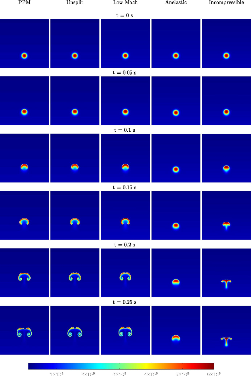
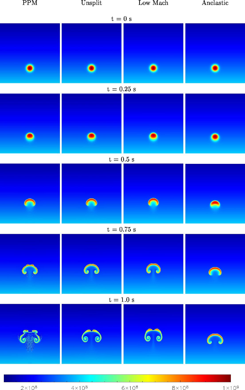
Figures 3 and 6 present comparisons of simulations using the low Mach number approach, two different discretizations of the fully compressible equation set, as well as the anelastic and incompressible equation sets. The low Mach number, anelastic and incompressible results are calculated using the projection method approach described in the previous section. The only differences in methodology occur in the coefficient of velocity in the projection, and in the construction of the buoyancy term. Each of these methods was run at a CFL number of 0.9 based on the maximum advection velocity.

Figure 3 shows the temperature evolution for $T_{\mathrm{max}}=6\times 10^{9}$ K. This corresponds to an Atwood number for the bubble of approximately 0.079. In this simulation, the bubble reaches a Mach number of about 0.2. In addition to the PPM and unsplit compressible solvers, traditional anelastic and incompressible solvers are shown for comparison. The low Mach number method closely tracks the two compressible solvers. The incompressible and anelastic results demonstrate the effects of their respective assumptions. The velocity constraint for the anelastic model is sufficiently accurate to capture the bubble rise, but because of the linearity of the density-temperature relationship in the anelastic approach, the buoyancy term is too small in the anelastic simulation. By contrast, the incompressible simulation contains the full buoyancy term but due to the incompressibility constraint the bubble cannot expand; consequently, it reaches neutral buoyancy at a much lower level and stops rising. We do not follow the bubbles past the point where nonlinear instabilities along the sides begin to dominate the evolution.

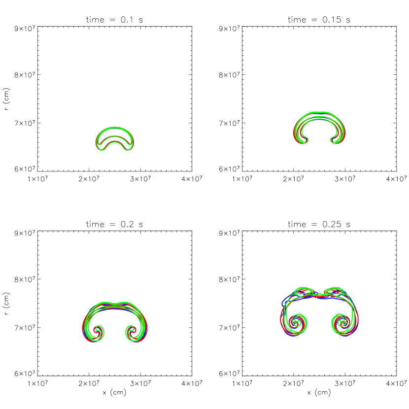
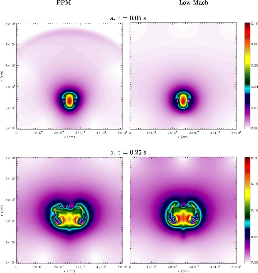
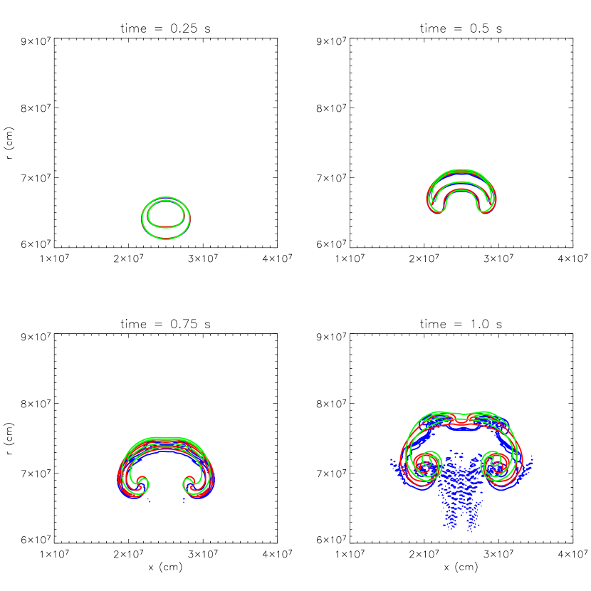
A more detailed comparison of the results from Figure 3 is provided in Figure 4, where temperature contours of the low Mach number solution are superimposed on temperature contours of the the unsplit and PPM solutions. Here we see a large degree of overlap, demonstrating that the bubbles have the same rise velocity and size independent of the algorithm. Figure 5 shows the Mach number of the PPM and low Mach number methods, further demonstrating the agreement between the two sets of results, with the exception of the unphysical loss of symmetry in the PPM simulation.

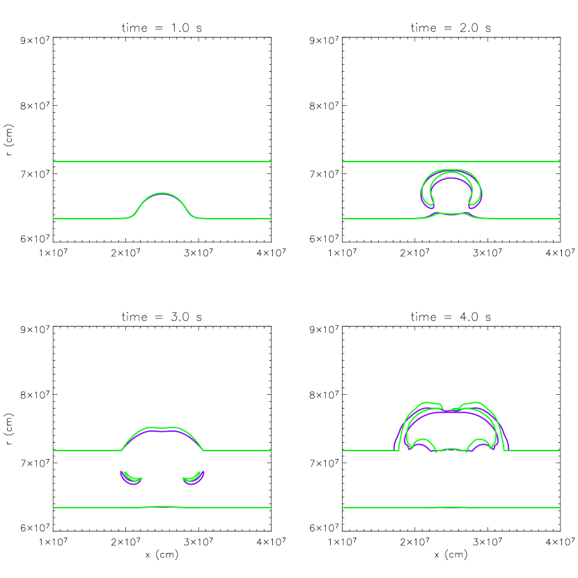
Figure 6 shows the temperature evolution for the lower peak temperature case, $T_{\mathrm{max}}=1\times 10^{9}$ K, and corresponding Atwood number of 0.0024. Over the course of this comparison, the Mach number remains below 0.05. Again, we observe the agreement between the low Mach number and compressible solvers, with the exception of the late-time breakdown of the PPM solution, indicated by the large amplitude temperature oscillations dominating the flow behind the bubble. These oscillations reflect the poor performance of operator split algorithms for very low speed flows.

A more detailed comparison of the results from Figure 6 is shown in Figure 7, again superimposing temperature contours from the low Mach number and compressible formulations. We again see good agreement, with the exception of the breakdown of PPM at late times.

Timings of the PPM and low Mach number code were made on a single processor (1.53 GHz Athlon MP) using the Intel 8.1 compilers. Both codes were compiled with the same compiler optimization flags: -O3 -ip -ipo. FLASH was set to run with $16\times 16$ zone blocks, instead of the default $8\times 8$ for better performance with uniform gridding. The $6\times 10^{9}$ K bubble required 2148 timesteps, taking 14200 s to evolve the bubble to $0.25$ s in simulation time. By comparison, the low Mach number solver took 246 timesteps and 1480 s, about an order of magnitude speed-up. For the $10^{9}$ K bubble, the PPM solver took 7842 timesteps, taking 52100 s to evolve the bubble for 1 s of simulation time, while the low Mach number solver took 252 timesteps and 1560 s. As expected, the performance gap increases as the Mach number decreases. The unsplit compressible algorithm takes approximately twice as much time to run as PPM, primarily due to the additional transverse Riemann solves required.

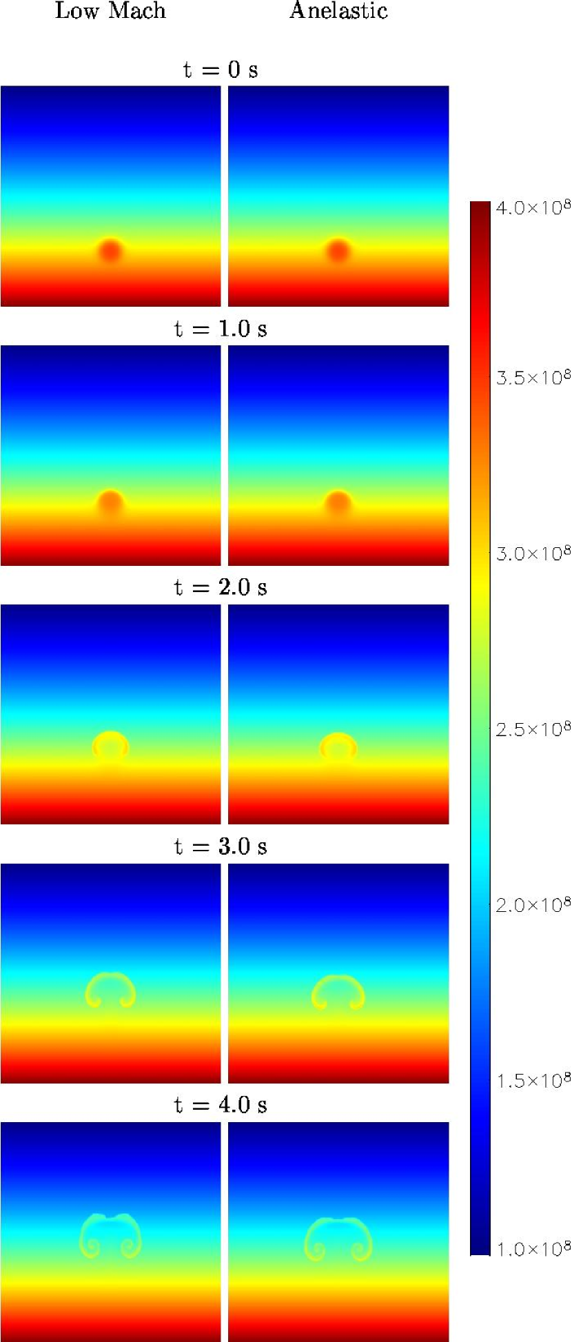
Finally, in Figures 8 and 9 we compare the low Mach number and anelastic models for a bubble with $T_{\mathrm{max}}=3.5\times 10^{8}$ K. This regime is inaccessible to the compressible formulation, with a peak Mach number during the calculation of $0.012$. We note that, as expected, as the Atwood number decreases the fidelity of the anelastic approximation improves.

The three cases presented in this section demonstrate successful application of the low Mach number approach, as well as failure of the compressible approach for low-speed flows, and failure of the anelastic approach for flows with large density or temperature variations. The low Mach number approach, like the other methods, has limits to its applicability. Specifically, as the flow speed, hence the Mach number, increases, typically the thermodynamic pressure will diverge from $p_{0}$ and the assumptions underlying the low Mach number approach will be violated. As with the anelastic model, numerical simulations using the low Mach number model will continue to yield what appear to be reasonable solutions even as the underlying assumptions are violated, but the solutions will no longer be physically relevant.

In the case of a bubble rise without heat sources, it is difficult to numerically demonstrate the failure of the low Mach number method even as the Mach number increases. However, the divergence of the low Mach number model from the compressible solution in the case of large Mach number will be discussed more thoroughly in the subsequent paper that discusses the behavior of the low Mach number model in the presence of heating.

5 Conclusions

We have introduced a new method for following low speed, stratified flows in astrophysical conditions and have demonstrated, through comparison with compressible and anelastic codes, that this algorithm performs well in the range of Mach number from near zero to about 0.2. The increased computational efficiency associated with a low Mach number formulation makes it an ideal tool for investigations of the convective/ignition phase of SNe Ia. However, to be applicable in this setting, a number of generalizations to the methodology will need to be developed. In particular, we will need to extend the the algorithm to include the effects of variation in composition, reactions and thermal conduction. In addition, once a flame is established it will be necessary to include sub-grid models for turbulent flame propagation that will enable the methodology to be used to simulate the evolution of the early phases of the explosion. These issues will be addressed in future work.

Appendix A Simplification of $\alpha$

In this appendix we derive a simplified expression for $\alpha$ introduced in equation 11. We refer to Chapter 9 of Cox & Giuli (1968) (CG, in this appendix), for a number of thermodynamic identities.

We begin by rewriting $h_{p}$, using

$$\frac{\partial h}{\partial\rho}\Bigg{|}_{T}=\frac{\partial h}{\partial p}\Bigg{|}_{T}\frac{\partial p}{\partial\rho}=h_{p}p_{\rho}\enskip.$$

with

$$h(\rho,T)=\frac{p(\rho,T)}{\rho}+e(\rho,T)\enskip.$$

Therefore,

$$h_{p}=p_{\rho}^{-1}\left\{{-\frac{p}{\rho^{2}}+\frac{p_{\rho}}{\rho}+e_{\rho}}\right\}=\frac{1}{\rho}\left(1-\frac{p}{\rho p_{\rho}}\right)+\frac{e_{\rho}}{p_{\rho}}\enskip.$$

Putting this into $\alpha$, we have

$$\alpha = -\frac{1}{\rho^{2}c_{p}p_{\rho}}\left[\left(1-\left(1-\frac{p}{\rho p_{\rho}}\right)-\rho\frac{e_{\rho}}{p_{\rho}}\right)p_{T}-\rho c_{p}\right]$$

$$= -\frac{1}{\rho p_{\rho}c_{p}}\left[\left(\frac{p}{\rho^{2}p_{\rho}}-\frac{e_{\rho}}{p_{\rho}}\right)p_{T}-c_{p}\right]\enskip.$$

For a generalized equation of state, there are three principal adiabatic exponents which relate the various differentials (d$p$, d$T$, and d$\rho$). For an ideal gas, they are all equivalent. Here, we use $\Gamma_{1}$ (CG eq. 9.88):

$$\Gamma_{1}\equiv\left(\frac{d\ln p}{d\ln\rho}\right)_{\mathrm{ad}}\enskip.$$

This is related to the ratio of specific heats, $\gamma$ via

$$\gamma=\frac{c_{p}}{c_{V}}=\frac{\Gamma_{1}}{\chi_{\rho}}\enskip,$$

(CG eq. 9.87) where

$$\chi_{\rho}\equiv\left(\frac{\partial\ln p}{\partial\ln\rho}\right)_{T}=\frac{\rho}{p}p_{\rho}$$

(CG eq. 9.82) is the “density exponent in the pressure equation of state.” For an ideal gas, $\chi_{\rho}=1$, and $\Gamma_{1}$ = $\gamma$. Taking all of this together, we see that

$$\frac{1}{\rho p_{\rho}}=\frac{\gamma}{\Gamma_{1}p}\enskip.$$

Putting this into our $\alpha$ expression,

$$\alpha=-\frac{\gamma}{\Gamma_{1}pc_{p}}\left[\left(\frac{p}{\rho^{2}p_{\rho}}-\frac{e_{\rho}}{p_{\rho}}\right)p_{T}-c_{p}\right]\enskip.$$ (A1)

Motivated by the ideal gas result that $\alpha=1/(\gamma p)$, we want to show that the quantity in the square brackets in equation (A1) reduces to $c_{V}$.

The specific heats are related by (CG eq. 9.84)

$$c_{p}-c_{V}=-\frac{E}{T}\left(\frac{\partial\ln E}{\partial\ln\rho}\right)_{T}\frac{\chi_{T}}{\chi_{\rho}}+\frac{p}{\rho T}\frac{\chi_{T}}{\chi_{\rho}}\enskip,$$ (A2)

The temperature exponent is defined as

$$\chi_{T}\equiv\left(\frac{\partial\ln p}{\partial\ln T}\right)_{\rho}=\frac{T}{p}p_{T}\enskip$$

(CG eq. 9.81), so equation (A2) simplifies to

$$c_{p}-c_{V} = -\frac{\rho}{T}e_{\rho}\frac{\chi_{T}}{\chi_{\rho}}+\frac{p}{\rho T}\frac{\chi_{T}}{\chi_{\rho}}$$

$$= -e_{\rho}\frac{p_{T}}{p_{\rho}}+\frac{p}{\rho^{2}}\frac{p_{T}}{p_{\rho}}\enskip,$$

which substitutes directly into equation (A1) to yield

$$\alpha=-\frac{\gamma}{\Gamma_{1}pc_{p}}\left[(c_{p}-c_{V})-c_{p}\right]=-\frac{\gamma}{\Gamma_{1}pc_{p}}\left[-c_{V}\right]=\frac{1}{\Gamma_{1}p}\enskip.$$

We note that $\Gamma_{1}$ varies slowly throughout the white dwarf and is a quantity that is already returned by the tabular equation of state.

Appendix B Derivation of $\beta$

We seek a function $\beta(z)$ such that

$$\frac{1}{\beta(z)}\nabla\cdot(\beta U)=(\nabla\cdot U)+\frac{1}{\Gamma_{1}p_{0}}U\cdot\nabla p_{0}\enskip.$$

We expand $\nabla\cdot(\beta U)=\beta(\nabla\cdot U)+U\cdot\nabla\beta$ and note that for the equality to hold we would need

$$\frac{1}{\beta(z)}U\cdot\nabla\beta=\frac{1}{\Gamma_{1}p_{0}}U\cdot\nabla p_{0}\enskip,$$

or

$$\frac{1}{\beta}w\beta^{\prime}=\frac{1}{\Gamma_{1}p_{0}}wp_{0}^{\prime}\enskip.$$

Since we want this to hold for all $w$, we are left with

$$\frac{\beta^{\prime}}{\beta}=\frac{p_{0}^{\prime}}{\Gamma_{1}p_{0}}\enskip.$$

We integrate this up from $z=0:$

$$\int_{0}^{z}\frac{\beta^{\prime}}{\beta}\,dz^{\prime}=\int_{0}^{z}\frac{d(\ln(\beta))}{dz}\,dz^{\prime}=\int_{0}^{z}(\frac{p_{0}^{\prime}}{\Gamma_{1}p_{0}})\,dz^{\prime}$$

so

$$\ln(\beta(z))-\ln(\beta(0))=\int_{0}^{z}(\frac{p_{0}^{\prime}}{\Gamma_{1}p_{0}})\,dz^{\prime}\enskip,$$

or

$$\beta(z)=\beta(0)\exp\left({\int_{0}^{z}(\frac{p_{0}^{\prime}}{\Gamma_{1}p_{0}})\,dz^{\prime}}\right)\enskip.$$

We note that this also can be written as the recursive relationship

$$\beta(z_{k})=\beta(z_{k-1})\exp\left({\int_{z_{k-1}}^{z_{k}}(-\frac{\rho_{0}g}{\Gamma_{1}p_{0}})\,dz^{\prime}}\right)\enskip,$$

exploiting the hydrostatic equilibrium of the base state. This equation is the one we use to numerically compute $\beta(z)$; we let $\beta(0)=\rho_{0}(0)$.

Figure 1: Illustration of the MAC-type grid showing the advective velocities ($u^{\mathrm{ADV}}$, $v^{\mathrm{ADV}}$) and $\phi^{\mathrm{MAC}}$ for the $(i,j)$ cell. An unsplit Godunov method is used to predict these advective velocities from the cell centered velocities ($u_{i,j}$, $v_{i,j}$) in the surrounding cells.

Figure 2: Initial model generated by the Kepler code (dotted) and uniformly gridded, constant gravity portion used in the bubble simulations (solid).

Figure 3: Bubble evolution for five different algorithms. Here, the peak temperature is $6\times 10^{9}$ K. We see good agreement between the two compressible codes (PPM and unsplit) and the low Mach number algorithm.

Figure 4: Detailed comparison of the temperature field for PPM (blue), the unsplit compressible algorithm (red), and the low Mach number algorithm (green), for the $6\times 10^{9}$ K perturbation. Contours are shown at $3\times 10^{9}$ and $4.5\times 10^{9}$ K.

Figure 5: Mach number comparison for the $6\times 10^{9}$ K bubble. At early times (a.), the PPM results show a sound wave from the initial perturbation just about to exit through the top of the domain. This is not present in the low Mach number case, as it filters sound waves. At late times (b.), the flow has attained a Mach number of almost 0.2 in places.

Figure 6: Bubble evolution for four different algorithms. Here, the peak temperature is $1\times 10^{9}$ K. As with the $6\times 10^{9}$ K case, the PPM, unsplit, and low Mach number results are in good agreement.

Figure 7: Detailed comparison of the temperature field for PPM (blue), the unsplit compressible algorithm (red), and the low Mach number algorithm (green), for the $1\times 10^{9}$ K perturbation. Contours are shown at $5\times 10^{8}$ and $7.5\times 10^{8}$ K.

Figure 8: Bubble evolution the low Mach number and anelastic algorithms, showing good agreement for the two different methods.. Here, the peak temperature is $3.5\times 10^{8}$ K.

Figure 9: Detailed comparison of the temperature field for the anelastic algorithm (purple) and the low Mach number algorithm (green), for the $3.5\times 10^{8}$ K perturbation. The contours are at $2.5\times 10^{8}$ and $3\times 10^{8}$ K

References

- Almgren et al. (1998) Almgren, A. S., Bell, J. B., Colella, P., Howell, L. H., & Welcome, M. L. 1998, Journal of Computational Physics, 142, 1
- Almgren et al. (2000) Almgren, A. S., Bell, J. B., & Crutchfield, W. Y. 2000, SIAM J. Sci. Comput., 22, 1139
- Almgren et al. (1996) Almgren, A. S., Bell, J. B., & Szymczak, W. G. 1996, SIAM J. Sci. Comput., 17, 358
- Batchelor (1953) Batchelor, G. K. 1953, Quart. J. R. meteor. Soc., 79, 224
- Bell et al. (1989) Bell, J. B., Colella, P., & Glaz, H. M. 1989, Journal of Computational Physics, 85, 257
- Bell et al. (1991) Bell, J. B., Colella, P., & Howell, L. H. 1991, in Proceedings of the Tenth AIAA Computational Fluid Dynamics Conference, AIAA, 360–367
- Bell et al. (2004) Bell, J. B., Day, M. S., Rendleman, C. A., Woosley, S. E., & Zingale, M. A. 2004, Journal of Computational Physics, 195, 677
- Bell & Marcus (1992) Bell, J. B., & Marcus, D. L. 1992, Journal of Computational Physics, 101, 334
- Botta et al. (1999) Botta, N., Klein, R., & Almgren, A. 1999, ENUMATH
- Boussinesq (1903) Boussinesq, J. 1903, Theorie analytique de la chaleur, Vol. 2 (Gauthier-Villars, Paris)
- Braginsky & Roberts (1995) Braginsky, S., & Roberts, P. H. 1995, Geophys. and Astrophys. Fluid Dynam., 79, 1
- Calder et al. (2002) Calder, A. C. et al. 2002, Astrophysical Journal Supplement, 143, 201
- Colella (1985) Colella, P. 1985, SIAM J. Sci. Stat. Comput., 6, 107
- Colella (1990) —. 1990, Journal of Computational Physics, 87, 171
- Colella & Glaz (1985) Colella, P., & Glaz, H. M. 1985, Journal of Computational Physics, 59, 264
- Colella & Woodward (1984) Colella, P., & Woodward, P. R. 1984, Journal of Computational Physics, 54, 174
- Cox & Giuli (1968) Cox, J. P., & Giuli, R. T. 1968, Principles of Stellar Structure, Vol. 1 (Cambridge University Press)
- Day & Bell (2000) Day, M. S., & Bell, J. B. 2000, Combust. Theory Modelling, 4, 535
- Durran (1989) Durran, D. R. 1989, Journal of Atmospheric Sciences, 46, 1453
- Dutton & Fichtl (1969) Dutton, J. A., & Fichtl, G. H. 1969, Journal of Atmospheric Sciences, 26, 241
- Fryxell et al. (2000) Fryxell, B. et al. 2000, Astrophysical Journal Supplement, 131, 273
- Gamezo et al. (2003) Gamezo, V. N., Khokhlov, A. M., Oran, E. S., Chtchelkanova, A. Y., & Rosenberg, R. O. 2003, Science, 299, 77
- Gilman & Glatzmaier (1981) Gilman, P. A., & Glatzmaier, G. A. 1981, Ap. J. Supp. Ser., 45, 335
- Glatzmaier (1984) Glatzmaier, G. A. 1984, J. Comp. Phys., 55, 461
- Gough (1969) Gough, D. O. 1969, Journal of Atmospheric Sciences, 26, 448
- Höflich & Stein (2002) Höflich, P., & Stein, J. 2002, Astrophysical Journal, 568, 779
- Harlow & Welch (1965) Harlow, F. H., & Welch, E. 1965, Phys. Fluids, 8, 2182
- Kuhlen et al. (2005) Kuhlen, M. Q., Woosley, S. E., & Glatzmaier, G. A. 2005, ApJ, in preparation
- Latour et al. (1976) Latour, J., Spiegel, E. A., Toomre, J., & Zahn, J.-P. 1976, Ap. J., 207, 233
- Lin (2005) Lin, D. J. 2005, PhD thesis, Field of Physics and Astronomy, Northwestern University
- Lipps (1990) Lipps, F. 1990, Journal of Atmospheric Sciences, 47, 1794
- Lipps & Hemler (1982) Lipps, F., & Hemler, R. 1982, Journal of Atmospheric Sciences, 39, 2192
- Lipps & Hemler (1985) —. 1985, Journal of Atmospheric Sciences, 42, 1960
- Majda & Sethian (1985) Majda, A., & Sethian, J. A. 1985, Comb. Sci. Tech., 42, 185
- Ogura & Phillips (1962) Ogura, Y., & Phillips, N. A. 1962, Journal of Atmospheric Sciences, 19, 173
- Pember et al. (1998) Pember, R. B., Howell, L. H., Bell, J. B., Colella, P., Crutchfield, W. Y., Fiveland, W. A., & Jessee, J. P. 1998, Comb. Sci. Tech., 140, 123
- Plewa et al. (2004) Plewa, T., Calder, A. C., & Lamb, D. Q. 2004, Astrophysical Journal, 612, L37
- Röpke & Hillebrandt (2005) Röpke, F. K., & Hillebrandt, W. 2005, A&A, 431, 635
- Rehm & Baum (1978) Rehm, R. G., & Baum, H. R. 1978, Journal of Research of the National Bureau of Standards, 83, 297
- Timmes & Swesty (2000) Timmes, F. X., & Swesty, F. D. 2000, ApJS, 126, 501
- Weaver et al. (1978) Weaver, T. A., Zimmerman, G. B., & Woosley, S. E. 1978, Astrophysical Journal, 225, 1021
- Wilhelmson & Ogura (1972) Wilhelmson, R., & Ogura, Y. 1972, Journal of Atmospheric Sciences, 29, 1295
- Woosley (2001) Woosley, S. E. 2001, Nuclear Physics A, 688, 9, Proceedings of Nuclei in the Cosmos 2000
- Woosley et al. (2004) Woosley, S. E., Wunsch, S., & Kuhlen, M. 2004, ApJ, 607, 921
- Wunsch & Woosley (2004) Wunsch, S., & Woosley, S. E. 2004, ApJ, 616, 1102
- Zingale et al. (2002) Zingale, M. et al. 2002, Astrophysical Journal Supplement, 143, 539