The dependence of clustering on galaxy properties

Abstract

We use a sample of $\sim 200,000$ galaxies drawn from the Sloan Digital Sky Survey (SDSS) with $0.01<z<0.3$ and $-23<M_{{}^{0.1}r}<-16$ to study how clustering depends on properties such as stellar mass ($M_{\ast}$), colour ($g-r$), 4000Å break strength (D₄₀₀₀), concentration index ($C$), and stellar surface mass density ($\mu_{\ast}$). Our measurements of $w_{p}(r_{p})$ as a function of r-band luminosity are in excellent agreement with previous two-degree Field Galaxy Redshift Survey and SDSS analyses. We compute $w_{p}(r_{p})$ as a function of stellar mass and we find that more massive galaxies cluster more strongly than less massive galaxies, with the difference increasing above the characteristic stellar mass $M^{\ast}$ of the Schechter mass function. We then divide our sample according to colour, 4000Å break strength, concentration and surface density. As expected, galaxies with redder colours, larger 4000Å break strengths, higher concentrations and larger surface mass densities cluster more strongly. The clustering differences are largest on small scales and for low mass galaxies. At fixed stellar mass, the dependences of clustering on colour and 4000 Å break strength are similar. Different results are obtained when galaxies are split by concentration or surface density. The dependence of $w_{p}(r_{p})$ on $g-r$ and D₄₀₀₀ extends out to physical scales that are significantly larger than those of individual dark matter haloes ($>5h^{-1}$ Mpc). This large-scale clustering dependence is not seen for the parameters $C$ or $\mu_{\ast}$. On small scales ($<1h^{-1}$ Mpc), the amplitude of the correlation function is constant for “young” galaxies with $1.1<$D${}_{4000}<1.5$ and a steeply rising function of age for “older” galaxies with D${}_{4000}>1.5$. In contrast, the dependence of the amplitude of $w_{p}(r_{p})$ on concentration on scales less than 1$h^{-1}$ Mpc is strongest for disk-dominated galaxies with $C<2.6$. This demonstrates that different processes are required to explain environmental trends in the structure and in the star formation history of galaxies.

1 Introduction

Our understanding of the large-scale structure of the Universe has come primarily from studies of redshift surveys of nearby galaxies. The two-point correlation function (2PCF) of galaxies has long served as the primary way of quantifying the clustering properties of galaxies in these surveys (for example, Peebles 1980). As the fundamental lowest order statistic, the 2PCF is simple to compute and provides a full statistical description for Gaussian fields. It can also be easily compared with the predictions of theoretical models. Such comparisons have led to the conclusion that the observations are not consistent with the predictions of the standard $\Lambda$CDM “concordance” model unless there is a scale-dependent bias in the distribution of galaxies relative to the dark matter (Jing, Mo & Börner 1998; Jenkins et al. 1998; Gross et al. 1998).

Benson et al. (2000a) clarified how the dependence of galaxy formation efficiency on halo mass could lead to just such a scale-dependent bias. On large scales, the bias in the galaxy distribution is related in a simple way to the bias in the distribution of dark haloes. On small scales, the amplitude and slope of the correlation function is determined by the interplay of a number of different effects, including the distribution of the number of galaxies that occupy a halo of given mass and the fact that the brightest galaxy in each halo is always located near the halo centre. These ideas have been further developed into the so-called “halo occupation distribution” (HOD) approach by many different authors (for example Jing, Mo & Börner 1998, Seljak 2000; Peacock & Smith 2000; Berlind & Weinberg 2002; Cooray & Sheth 2002; Yang, Mo & van den Bosch 2003).

The HOD approach enables one to understand why the correlation function of $L^{\ast}$ galaxies is close to a power law over nearly four orders of magnitude in amplitude in a flat, $\Omega_{0}=0.3$ CDM universe. However, an important corollary is that the clustering properties of galaxies ought to depend strongly on galaxy colour, star formation rate and morphology, because the halo occupation distributions of galaxies are predicted to depend sensitively on these properties (see for example Kauffmann, Nusser & Steinmetz 1997; Kauffmann et al. 1999; Benson et al. 2000b).

The fact that the measured correlations of galaxies differ according to type has been known for almost three decades. Davis & Geller (1976) computed angular correlations for galaxies in the Uppsala Catalog and showed that elliptical-elliptical correlations were characterized by a power law with steeper slope than spiral-spiral correlations. Dressler (1980) quantified this as a relation between galaxy type and local galaxy density, with an increasing elliptical and S0 population and a corresponding decrease in spirals in the densest environments.

The large redshift surveys assembled in recent years, e.g. 2dFGRS and SDSS, have provided angular positions and redshifts for samples of hundreds of thousands of galaxies and have allowed the dependence of clustering on galaxy properties to be studied with unprecedented accuracy. These studies have established that the clustering of galaxies in the local Universe depends on a variety of factors, including luminosity (Norberg et al. 2001, Zehavi et al. 2002, Zehavi et al. 2005), colour (Zehavi et al. 2002, Zehavi et al. 2005), concentration (Zehavi et al. 2002, Goto et al. 2003), and spectral type (Norberg et al. 2002, Budavári et al. 2003, Madgwick et al. 2003). These studies have revealed that galaxies with red colours, bulge-dominated morphologies and spectral types indicative of old stellar populations reside preferentially in dense regions (Zehavi et al. 2005 and references therein, hereafter Z05). Furthermore, luminous galaxies cluster more strongly than less luminous galaxies, with the luminosity dependence becoming more significant for galaxies brighter than $L^{\ast}$ (the characteristic luminosity of the Schechter [1976] function). When galaxies are divided by colour, redder galaxies show a higher amplitude and steeper correlation function at all luminosities.

In order to interpret these clustering dependencies in the framework of galaxy formation models, it is useful to express the clustering results in terms of physical quantities such as galaxy mass, size and mean stellar age, instead of more traditional quantities such as luminosity or colour. Galaxy luminosity does not necessarily correlate very closely with stellar mass (the dominant baryonic component in all but the smallest galaxies). Both luminosity and colour are subject to strong dependences on the fraction of young stars in the galaxy and on its dust content. These effects also complicate comparisons between the clustering of low redshift and high redshift galaxies. It is now known that the star formation rates in galaxies evolve very strongly as a function of redshift. As a result, if one measures a change in clustering amplitude at fixed luminosity, it is not simple to ascertain which part of the effect is caused by the evolution in the stellar mass-to-light ratio ($M_{\ast}/L$) and which part by a change in the halo occupation distributions at higher redshift.

In this paper we study the dependence of galaxy clustering on both luminosity and stellar mass using a large sample of galaxies drawn from the Sloan Digital Sky Survey. We then probe the dependence on other physical parameters, including colour ($g-r$), 4000Å break strength (D₄₀₀₀), concentration parameter ($C$)and stellar surface mass density ($\mu_{\ast}$). The first two quantities, i.e. $g-r$ and D₄₀₀₀, are parameters associated with the recent star formation history of the galaxy (D₄₀₀₀ is expected to be less sensitive to dust attenuation effects than colour), whereas the other two are related to galaxy structure. We first describe the observational samples used for the analysis. In §3 we outline our method of measuring the 2PCF from large redshift surveys. The results are described in §4 and summarized in the final section.

Throughout this paper, We assume a cosmological model with the density parameter $\Omega_{0}=0.3$ and the cosmological constant $\Lambda_{0}=0.7$. To avoid the $-5\log_{10}h$ factor, the Hubble’s constant $h=1$, in units of $100\,{\rm{km\,s^{-1}}}{\rm Mpc}^{-1}$, is assumed throughout this paper when computing absolute magnitudes. In this paper, the quantities with a superscript asterisk are those at the characteristic luminosity/mass (e.g. characteristic luminosity $L^{\ast}$), whereas the quantities with a subscript asterisk refer to quantities associated with the stars in a galaxy (e.g. stellar mass $M_{\ast}$).

Figure 1: The results of a computation that we carried out to see out to what redshift a given mass in stars with maximum possible $M_{\ast}/L$ would be detected. This assumes a 13 Gyr stellar population and Bruzual & Charlot models.

Figure 2: Shown in the upper panel are the contours of number density of galaxies in the plane of stellar mass vs luminosity. The black lines are for the data and the red are reconstructed using the Gaussian functions that best fit the stellar mass distribution in 282 different luminosity intervals. The contour levels are increased by factors of 2 from the lowest (15 $[0.2mag]^{-1}[0.2\log_{10}M_{\odot}]^{-1}$) to the highest (7680 $[0.2mag]^{-1}[0.2\log_{10}M_{\odot}]^{-1}$). The lower panel shows examples of the Gaussian distributions. Histograms show the data and solid lines the best-fits. $N_{0}$ is the Gaussian height. The corresponding centers (blue points) and widths (errorbars) of the Gaussians are shown in the upper panel.

2 Observational Samples

2.1 NYU-VAGC

The Sloan Digital Sky Survey (SDSS) is the most ambitious optical imaging and spectroscopic survey to date. The survey goals are to obtain photometry of a quarter of the sky and spectra of nearly one million objects. Imaging is obtained in the u, g, r, i, z bands (Fukugita et al. 1996; Smith et al. 2002; Ivezić et al. 2004) with a special purpose drift scan camera (Gunn et al. 1998) mounted on the SDSS 2.5 meter telescope at Apache Point Observatory. The imaging data are photometrically (Hogg et al. 2001) and astrometrically (Pier et al. 2003) calibrated, and used to select stars, galaxies, and quasars for follow-up fibre spectroscopy. Spectroscopic fibres are assigned to objects on the sky using an efficient tiling algorithm designed to optimize completeness (Blanton et al. 2003b). The details of the survey strategy can be found in (York et al. 2000) and an overview of the data pipelines and products is provided in the Early Data Release paper (Stoughton et al. 2002).

The large areal coverage and moderately deep survey limit (a mean redshift of $\sim 0.1$ for galaxies in the main spectroscopic sample) make the SDSS ideal for studying large-scale structure and the characteristics of galaxy populations in the local Universe. The SDSS covers two regions on the sky, one in the northern Galactic cap (NGC) and another in the southern Galactic cap (SGC). In the SGC, three stripes are observed, one along the celestial equator and the other two north and south of the equator. The NGC lies mostly above Galactic latitude 30^∘, but its footprint is adjusted slightly to lie within the minimum of the Galactic extinction contours (Schlegel, Finkbeiner, & Davis 1998), resulting in an elliptical survey region (York et al. 2000). Currently the survey in the NGC consists of two separate regions, one along the celestial equator (hereafter NGCE) and another off the equator (hereafter NGCO).

In this paper we use the New York University Value Added Catalog (NYU-VAGC), which is a catalog of local galaxies (mostly below $z\approx 0.3$) constructed by Blanton et al. (2005a) based on the SDSS Data Release Two (DR2, Abazajian et al. 2004). Earlier proprietary versions of this catalog have formed the basis of many SDSS investigations of the power spectrum, correlation function, and luminosity function of galaxies. The current version of the NYU-VAGC consists of 693,319 photometric objects (3514 deg²); 343,568 of these have redshift determinations (2627 deg²), with about 85% completeness. This small subset of the full SDSS catalog contains all of the information necessary for analyzing the SDSS spectroscopic survey at the catalog level. Compared with the catalogs distributed by the SDSS DR2 Archive Servers, the NYU-VAGC is photometrically calibrated in a more consistent way, reducing systematic calibration errors across the sky from $\sim$ 2% to about $\sim$ 1%. It is therefore more appropriate for statistical studies of galaxy peoperties, galaxy clustering, and galaxy evolution. The NYU-VAGC is described in detail in Blanton et al. (2005a).

2.2 Physical quantities

The rich stellar absorption-line spectrum of a typical SDSS galaxy provides unique information about its stellar content and dynamics. Kauffmann et al. (2003a) presented a method for using this information to estimate the stellar masses of galaxies. The amplitude of the 4000 Å break (the narrow version of the index defined in Balogh et al. 1999) and the strength of the H$\delta$ absorption line (the Lick $H\delta_{A}$ index of Worthey & Ottaviani 1997) were used as diagnostics of the stellar populations of the galaxies. Both indices were corrected for the observed contributions of the emission lines in their bandpasses. From a library of 32,000 model star formation histories, the measured D₄₀₀₀ and $H\delta_{A}$ indices were used to obtain a maximum likelihood estimate of the $z$-band $M_{\ast}/L$ for each galaxy. By comparing the colour predicted by the best-fit model to the observed colour of the galaxy, the attenuation of the starlight due to dust could be estimated.

The SDSS imaging data provide the basic structural parameters that are used in this analysis. The $z$-band absolute magnitude, combined with the estimated values of $M_{\ast}/L$ and dust attenuation $A_{z}$ yield the stellar mass ($M_{\ast}$). The half-light radius in the $z$-band and the stellar mass yield the effective stellar surface mass-density ($\mu_{\ast}=M_{\ast}/2\pi r_{50,z}^{2}$, in unit of $h^{2}M_{\odot}/$kpc²). As a proxy for Hubble type we use the SDSS “concentration” parameter $C$, which is defined as the ratio of the radii enclosing 90% and 50% of the galaxy light in the $r$ band (see Stoughton et al. 2002). Strateva et al. (2001) find that galaxies with $C>$ 2.6 are mostly early-type galaxies, whereas spirals and irregulars have 2.0 $<C<$ 2.6.

The reader is referred to Kauffmann et al. (2003a) for a more detailed description of the methodology used to derive the stellar masses used in this paper. An analysis of how the physical properties of galaxies correlate with mass is presented in Kauffmann et al. (2003b). All the parameters used in this paper are available publically at http://www.mpa-garching.mpg.de/SDSS/ (see also Brinchmann et al. 2004).

2.3 Sample selection

Table 1: Flux-limited samples selected according to luminosity/stellar mass

		Number of Galaxies					Percentage in Subsamplesa
Sample	$M_{{}^{0.1}r}$	SGC	NGCO	NGCE	Total		$g-r$	D4000	$C$	$\log_{10}\mu_{\ast}$
L1………..	$[-17.0,-16.0)$	458	548	608	1614		27.2%	41.7%	90.7%	48.0%
L2………..	$[-17.5,-16.5)$	735	1261	1115	3111		26.2%	32.2%	82.9%	43.4%
L3………..	$[-18.0,-17.0)$	1257	2301	1695	5253		27.3%	27.6%	74.2%	41.4%
L4………..	$[-18.5,-17.5)$	2130	3808	2693	8631		31.0%	26.3%	67.0%	44.2%
L5………..	$[-19.0,-18.0)$	3657	6391	4366	14414		36.6%	29.3%	60.5%	49.3%
L6………..	$[-19.5,-18.5)$	6532	10754	8582	25868		43.9%	36.4%	55.9%	56.3%
L7………..	$[-20.0,-19.0)$	10349	16788	15740	42877		49.1%	42.6%	54.3%	61.5%
L8………..	$[-20.5,-19.5)$	14804	24688	22879	62371		51.9%	46.9%	54.9%	63.7%
L9………..	$[-21.0,-20.0)$	18460	31997	27530	77987		52.9%	51.2%	56.6%	61.9%
L10……….	$[-21.5,-20.5)$	17717	31010	25376	74103		53.4%	56.4%	58.9%	54.7%
L11……….	$[-22.0,-21.0)$	12140	20647	16252	49039		55.9%	62.7%	64.3%	41.1%
L12……….	$[-22.5,-21.5)$	5384	8895	6876	21155		61.1%	70.5%	72.6%	23.3%
L13……….	$[-23.0,-22.0)$	1267	2097	1674	5038		64.8%	78.0%	76.3%	7.20%
Sample	$\log_{10}M_{\ast}$
M1………..	$[9.0,9.5)$	1686	3230	2325	7241		14.7%	14.5%	55.8%	26.3%
M2………..	$[9.5,10.0)$	4086	6695	5237	16018		23.8%	19.8%	44.3%	36.5%
M3………..	$[10.0,10.5)$	9757	15528	14275	39560		43.4%	38.8%	49.5%	56.3%
M4………..	$[10.5,11.0)$	17340	30519	26423	74282		55.3%	53.1%	58.9%	63.8%
M5………..	$[11.0,11.5)$	12475	21213	16671	50359		65.5%	70.0%	70.5%	51.7%
M6………..	$[11.5,12.0)$	1183	2082	1603	4868		71.7%	83.7%	78.1%	17.3%
a Percentage of objects in subsample with larger value of physical quantities.

Table 2: Volume-limited samples

			Number of Galaxies
Sample	$M_{{}^{0.1}r}$	$z$	SGC	NGCO	NGCE	Total
VL1……….	$[-18.0,-17.0)$	$(0.01,0.03)$	675	1011	1016	2702
VL2……….	$[-19.0-18.0)$	$(0.02,0.04)$	986	1776	1433	4195
VL3……….	$[-20.0,-19.0)$	$(0.03,0.07)$	4510	7135	4514	16159
VL4……….	$[-21.0,-20.0)$	$(0.04,0.07)$	2202	3275	2076	7553
VL5……….	$[-21.0,-20.0)$	$(0.04,0.10)$	6886	10021	10772	27679
VL6……….	$[-22.0,-21.0)$	$(0.07,0.16)$	5566	9446	8335	23347
VL7……….	$[-23.0,-22.0)$	$(0.10,0.23)$	705	1146	874	2725
Sample	$\log_{10}M_{\ast}$	$z$	SGC	NGCO	NGCE	Total
VM1……….	$[9.0,9.5)$	$(0.015,0.045)$	1195	2190	1624	5009
VM2……….	$[9.5,10.0)$	$(0.020,0.075)$	3368	5622	4020	13010
VM3……….	$[10.0,10.5)$	$(0.025,0.100)$	8039	12530	11865	32434
VM4……….	$[10.5,11.0)$	$(0.040,0.140)$	14324	24403	22035	60762
VM5……….	$[11.0,11.5)$	$(0.070,0.200)$	10343	17393	14065	41801

In this paper, all the three regions in NYU-VAGC, i.e. NGCE, NGCO and SGC, are considered. Statistics are measured separately for the three regions but the results are always presented for the whole survey by combining the results in these regions.

We first select all NYU-VAGC galaxies with extinction corrected Petrosian magnitude $14.5<r<17.77$. The bright limit is so chosen because the SDSS becomes incomplete for bright galaxies with large angular size, whereas the faint limit corresponds to the magnitude limit of the Main galaxy sample in SDSS. Further criteria for galaxies to be included in our analysis are, 1) they are identified as galaxies from the Main sample (see Blanton et al. 2005a for a detailed description), 2) they lie within the redshift range $0.01\leq z\leq 0.3$ and the absolute magnitude range $-23<M_{{0.1}_{r}}<-16$. Here $M_{{0.1}_{r}}$ is the $r$-band absolute magnitude corrected to its $z=0.1$ value using the $K-$correction code (kcorrect v3_1b) of Blanton et al. (2003a) and the luminosity evolution model of Blanton et al. (2003c). Our resulting sample includes a total of 196238 galaxies.

The galaxies are then divided into a variety of different subsamples. We create 13 subsamples according to absolute magnitude, ranging from $M_{{}^{0.1}r}=-16$ to $M_{{}^{0.1}r}=-23$. Each sample includes galaxies in an absolute magnitude interval of 1 magnitude, with successive subsamples overlapping by 0.5 magnitude. Details are given in Table 1 (Samples L1-L13).

Table 3: Flux-limited samples selected according to physical quantities

		Number of Galaxies
Sample	$g-r$	SGC	NGCO	NGCE	Total
c1………..	$[0.2,0.5)$	2348	3674	3383	9405
c2………..	$[0.3,0.6)$	5798	9511	8411	23720
c3………..	$[0.4,0.7)$	9350	15713	13647	38710
c4………..	$[0.5,0.8)$	11464	19502	16925	47891
c5………..	$[0.6,0.9)$	14206	23717	21363	59286
c6………..	$[0.7,1.0)$	16557	28504	25476	70537
c7………..	$[0.8,1.1)$	13188	22679	20229	56096
c8………..	$[0.9,1.2)$	6979	12617	10714	30310
Sample	D4000	SGC	NGCO	NGCE	Total
D1………..	$[1.0,1.3)$	3807	6245	5309	15361
D2………..	$[1.1,1.4)$	7755	12868	11050	31673
D3………..	$[1.2,1.5)$	10333	17565	15065	42963
D4………..	$[1.3,1.6)$	9900	17010	14561	41471
D5………..	$[1.4,1.7)$	8281	14296	12192	34769
D6………..	$[1.5,1.8)$	7762	13298	11527	32587
D7………..	$[1.6,1.9)$	9090	15716	13874	38680
D8………..	$[1.7,2.0)$	9902	17143	15622	42667
D9………..	$[1.8,2.1)$	8048	13776	12805	34629
D10……….	$[1.9,2.2)$	4274	7044	6916	18234
D11……….	$[2.0,2.3)$	1108	1654	1766	4528
Sample	$C$	SGC	NGCO	NGCE	Total
C1………..	$[1.5,2.1)$	3372	5677	4783	13832
C2………..	$[1.7,2.3)$	7457	12720	10708	30885
C3………..	$[1.9,2.5)$	11027	19257	16399	46683
C4………..	$[2.1,2.7)$	12504	22439	19232	54175
C5………..	$[2.3,2.9)$	13007	23332	20616	56955
C6………..	$[2.5,3.1)$	12841	22119	19967	54927
C7………..	$[2.7,3.3)$	10620	17116	15881	43617
C8………..	$[2.9,3.5)$	6533	9827	9227	25587
C9………..	$[3.1,3.7)$	2647	3752	3580	9979
Sample	$\log_{10}\mu_{\ast}$	SGC	NGCO	NGCE	Total
$\mu$1………..	$[8.00,8.50)$	2006	3415	2818	8239
$\mu$2………..	$[8.25,8.75)$	5430	9447	7989	22866
$\mu$3………..	$[8.50,9.00)$	9960	17419	15139	42518
$\mu$4………..	$[8.75,9.25)$	14166	24865	21974	61005
$\mu$5………..	$[9.00,9.50)$	13593	23073	20834	57500
$\mu$6………..	$[9.25,9.75)$	7015	10908	10044	27967
$\mu$7………..	$[9.50,10.0)$	1495	2065	1819	5379

Similarly, the galaxies are divided into 6 subsamples according to $\log_{10}M_{\ast}$ (M1-M6 in Table 1). We do not consider galaxies with $\log_{10}M_{\ast}<9$, because the volume of the survey over which such systems can be detected is extremely small. This is illustrated in Fig.1, where we plot the maximum redshift out to which a galaxy of mass $M_{\ast}$ with maximal $M_{\ast}/L$ would be detected in the survey. This calculation assumes a 13 Gyr single-age stellar population and is based on the Bruzual & Charlot (2003) models. At stellar masses below $10^{9}M_{\odot}$, the oldest galaxies are only visible at $z<0.03$. For galaxies with masses less than $10^{8}M_{\odot}$ the maximum redshift is well below 0.02.

To compare our results to previous work, we have also constructed volume-limited subsamples (see Table 2), including subsamples that are volume-limited in luminosity (Sample VL1-VL7) and in stellar mass (Sample VM1-VM5). The absolute magnitude ranges and redshift ranges used for selecting subsamples VL1-VL7 are the same as in Z05.

As will be described in Section 4.4, we further divide each luminosity and stellar mass subsample into red and blue, high D₄₀₀₀ and low D₄₀₀₀, low concentration and high concentration, low density and high density subsamples by fitting the distributions of these parameters using bi-Gaussian functions. These subsamples are also listed in Table 1. It is also interesting to investigate how clustering varies as a function of colour/D₄₀₀₀/concentration/surface density at fixed stellar mass. To this end, we select a sample of galaxies with stellar masses in the range of $10<\log_{10}M_{\ast}<11$, and divide the galaxies into subsamples according to their $g-r$ colours (Sample c1-c8), D₄₀₀₀ values (Sample D1-D12), concentrations (Sample C1-C10) and surface mass densities (Sample $\mu$1-$\mu$6). The details of these subsamples are given in Table 3.

3 Clustering Measures

In this section, we outline our method for measuring the galaxy two-point correlation function for a flux-limited sample of galaxies. We begin by describing our methods for constructing random samples. We then describe how we correct for the effect of fibre collisions. Finally, we describe the 2PCF estimator and how measurement errors are calculated.

3.1 Constructing Random samples

In order to use galaxy surveys in a statistically meaningful way, we need to have complete knowlege of their selection effects. A detailed account of the observational selection effects accompanies the NYU-VAGC release. The survey geometry is expressed as a set of disjoint convex spherical polygons, defined by a set of “caps”. This methodology was developed by Andrew Hamilton to deal accurately and efficiently with the complex angular masks of galaxy surveys (Hamilton & Tegmark 2002). The advantage of using this method is that it is easy to determine whether a point is inside or outside a given polygon (Tegmark, Hamilton & Xu 2002). The redshift sampling completeness is then defined as the number of galaxies with redshifts divided by the total number of spectroscopic targets in the polygon. The completeness is thus a dimensionless number between 0 and 1, and it is constant within each of the polygons. The limiting magnitude in each polygon is also provided (it changes slightly across the survey region).

We have constructed separate random catalogues for each of the three regions of sky. These catalogues are designed to include all observational selection effects and are constructed as follows. First, we select a spatial volume that is sufficiently large to contain the survey sample. Then we randomly distribute points within the volume and eliminate the points that are outside the survey boundary. Adopting the same magnitude limits as in the observational sample, we select random galaxies and we use the luminosity function derived by Blanton et al. (2003c) to assign to each of these galaxies an apparent and an absolute magnitude (appropriately $K$ and $E$-corrected, see §2.3).

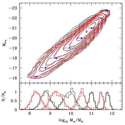
Since we will estimate the correlation function as a function of stellar mass, we also need to assign a mass to each point in the random sample. One way to do this is to use the observed relation between luminosity and stellar mass derived directly from our sample. The black lines in the top panel of Fig.2 show contours of the number density of galaxies in the plane of absolute magnitude vs stellar mass. It can be seen from the histograms in the bottom panel of this figure that at fixed luminosity, the distribution of the stellar mass of galaxies is well described by a Gaussian, with the width of the Gaussian decreasing at higher luminosities.

We have divided the galaxies in our sample into 282 subsamples separated by 0.03 mag in $M_{{}^{0.1}r}$. The bin size was chosen so that each subsample contained at least 500 galaxies. The stellar mass distribution in each subsample is fitted with a Gaussian and the solid lines in the bottom panel of Fig.2 show examples of these fits for several luminosity intervals. To test the quality of the fits, we randomly assign each galaxy a new stellar mass using the Gaussian fits. The red lines in the top panel of Fig.2 show contours of the number density distribution that is predicted by this parametrization. The recovered distribution is a good match to the observations except in the region corresponding to luminous galaxies with low $M_{\ast}/L$s, where the method tends to overpredict the masses.

We now introduce a more general method, which should still be applicable even when the relation between galaxy luminosity and the physical property under investigation is not well fit by a Gaussian and is subject to redshift-dependent selection biases. Our method takes the observed sample and randomly re-assigns the position of each galaxy on the sky, while keeping the redshift, absolute magnitude, stellar mass, and any other physical quantities fixed. The spectroscopic incompleteness at each sky position is imposed for the random points as in the observed sample. To get a random catalogue as large as possible, we repeat the above procedure for 20 times using different random number seeds. In this way, all possible redshift-dependent selection biases are automatically taken into account, and it is only the sky position that is randomized. This method is valid only when the sample is a wide-angle survey and the variation of its limiting magnitudes is small across the survey region, both of which are valid in the SDSS. For very large-area surveys such as the SDSS, randomizing the sky positions should be sufficient to break the coherence of the large scale structures in the survey. In the next section we will use random catalogues constructed using both methods and we will show that the measured projected correlation functions are in good agreement (see Fig.3).

3.2 Volume Corrections

When computing correlation functions as a function of stellar mass, it is important to note that at a given stellar mass $M_{\ast}$, galaxies with lower $M_{\ast}/L$ will be detected out to higher redshifts. A mass-selected sample will thus be biased to galaxies with younger populations and this may lead to systematic errors when computing the correlation function at fixed $M_{\ast}$. In this paper, we correct for this $M_{\ast}/L$ bias by computing a weighted correlation function: each galaxy pair is weighted by the inverse of the volume over which both galaxies can be detected in the survey. This is similar to the $1/V_{max}$ correction that one makes when computing a mass function or luminosity function. The same volume weighting must also be applied to the random catalogue. It is very simple to apply the same technique to the catalogues constructed by randomizing the sky positions, so this will be our method of choice when estimating correlations as a function of stellar mass.

In order to compute the volumes over which galaxies can be detected, we have computed $z_{min}$ and $z_{max}$ for each galaxy in the sample, where $z_{min}$ is defined as the redshift where the galaxy has an $r$-band magnitude of 14.5 and $z_{max}$ is the redshift where the galaxy has an $r$-band magnitude of 17.77. These are derived using the kcorrect code of Blanton et al. (2003c).

Figure 3: Projected 2PCF $w_{p}(r_{p})$ in different luminosity intervals (Sample L3, L5, L7, L9, L11 and L13 in Table 1). When measuring 2PCFs, two methods are used to construct random samples (see §3.1). The black lines are for the standard method and the red lines are for the method in which the sky positions are randomized (see the text for a detailed description). In each panel, the blue line is the line corresponding to $\xi(r)=(r/5h^{-1}\mbox{Mpc})^{-1.8}$.

3.3 Correction for fibre collisions

In the SDSS survey, two galaxies closer than $55^{\prime\prime}$ (corresponding to $\sim 100\>{h^{-1}{\rm kpc}}$ at the median redshift of our sample) cannot be assigned fibres simultaneously on one spectroscopic plate. If these fibre “collisions” are not taken into account, the real-space (or projected) 2PCF will be systematically underestimated at small separations. In earlier work (e.g. Zehavi et al. 2002, Tegmark et al. 2004), a correction was made by simply assigning to each galaxy affected by a collision the same redshift as its nearest spectroscopically-targeted neighbour on the sky. Zehavi et al. (2002) have performed extensive tests of this procedure and have shown that it works well for $r_{p}>0.1\>h^{-1}{\rm{Mpc}}$. Tegmark et al. (2004) also find no evidence that fibre collisions are boosting their measured power spectrum on the smallest scales they probe ($k\sim 0.3$ $h$ Mpc^-1 ).

In this paper, we use a different method for correcting for fibre collisions. We measure the angular 2PCF both for the spectroscopic samples and for the parent photometric sample from which they were drawn; the effect of fibre collisions can then be estimated and corrected for by comparing the two correlation functions. A similar method has been used in 2dF clustering analyses by Hawkins et al. (2003).

Here we briefly sumarize our method, which will be described in more detail in a separate paper (Li et al., in preparation). We calculate the angular 2PCF for the photometric sample ($w_{p}(\theta)$) and for the spectroscopic sample ($w_{z}(\theta)$). The quantity

$$F(\theta)=\frac{w_{z}(\theta)+1}{w_{p}(\theta)+1},$$ (1)

can then be used to account for the effect of fibre collisions. For each data-data pair, we calculate the angular distance $\theta$ between the two members of the pair and weight this pair by $1/F(\theta)$ when estimating the pair counts. If this correction is not applied, both $w(\theta)$ and $w_{p}(r_{p})$ exhibit a strong “rollover” in amplitude on small scales. Once the correction is applied, this feature disappears. In the rest of our analysis, we will always include the $1/F(\theta)$ weighting in the measurements of the correlation functions. Since the effect of fiber collisions is expected to be independent of galaxy property, we will not derive the correction function $F(\theta)$ for each individual galaxy sample, but choose to derive it from the whole sample and then apply it to our subsamples.

3.4 Estimator of the Correlation Function and errors

In this paper, the 2PCFs are measured in equal logarithmic bins of $r_{p}$ and in equal linear bins of $\pi$, using the Hamilton (1993) estimator,

$$\xi(r_{p},\pi)=\frac{4DD(r_{p},\pi)RR(r_{p},\pi)}{[DR(r_{p},\pi)]^{2}}-1.$$ (2)

Here $r_{p}$ and $\pi$ are the separations perpendicular and parallel to the line of sight; $DD(r_{p},\pi)$ is the count of data-data pairs with perpendicular separations in the bins $\log_{10}r_{p}\pm 0.5\Delta\log_{10}r_{p}$ and with radial separations in the bins $\pi\pm 0.5\Delta\pi$; $RR(r_{p},\pi)$ and $DR(r_{p},\pi)$ are the counts of random-random and data-random pairs, respectively. The reason why we choose different bins for $r_{p}$ and $\pi$ is the fact that $\xi(r_{p},\pi)$ decreases rapidly as a function of $r_{p}$, but remains constant as a function of $\pi$ on small scales. Following standard practice, we estimate the projected two-point correlation function $w_{p}(r_{p})$ by,

$$w_{p}(r_{p})=2\int_{0}^{\infty}\xi(r_{p},\pi)d\pi=2\sum_{i}\xi(r_{p},\pi_{i})\Delta\pi_{i}.$$ (3)

Here the summation for computing $w_{p}(r_{p})$ runs from $\pi_{1}=0.5\>h^{-1}{\rm{Mpc}}$ to $\pi_{40}=39.5\>h^{-1}{\rm{Mpc}}$, with $\Delta\pi_{i}=1\>h^{-1}{\rm{Mpc}}$. The projected correlation function $w_{p}(r_{p})$ is directly related to the real-space CF $\xi(r)$ by a simple Abel transform of $\xi(r)$. Commonly, $w_{p}(r_{p})$ is modelled by a power law

$$w\left(r_{p}\right)=Ar_{p}^{1-\gamma}.$$ (4)

Then $\xi(r)$ is also a power law

$$\xi(r)=(r_{0}/r)^{\gamma}$$ (5)

with

$$r_{0}^{\gamma}=\frac{A\Gamma(\gamma/2)}{\Gamma(1/2)\Gamma[(\gamma-1)/2]},$$ (6)

where $\Gamma(x)$ is the Gamma function. However, the parametrization of the correlation function using only $r_{0}$ and $\gamma$ does not provide sufficient information to recover the full observational results unless the correlation function is a pure power law on all scales. Our results (see below) show that this is not the case. The departures of $w(r_{p})$ from a pure power law have also been discussed in previous papers (e.g. Zehavi et al. 2004). We have thus chosen to present our results in terms of the measured amplitude of $w_{p}(r_{p})$ on different physical scales. We also tabulate the correlation functions so that our readers can recover them accurately. A detailed description of these tables (Tables 5 and 6) is given in the Appendix. The tables themselves are available in electronic form at http://www.mpa-garching.mpg.de/^∼leech/papers/clustering/.

The errors on the clustering measurements are estimated using the bootstrap resampling technique (Barrow, Bhavsar, & Sonoda 1984). We generate 100 bootstrap samples from the observations and compute the correlation functions for each sample using the weighting scheme (but not the approximate formula) given by Mo, Jing, & Börner (1992). The errors are then given by the scatter of the measurements among these bootstrap samples. The tests in Jing, Mo & Börner (1998) using mock samples showed that the bootstrap errors are comparable (within a factor of 2) to the scatter among different mock samples, thus proving that the error estimates are robust.

Figure 4: Amplitude of the projected 2PCF $w_{p}(r_{p})$ as a function of luminosity (Samples L1-L13) at $r_{p}=$0.2, 1, 5, and 10 $h^{-1}$ Mpc.

Figure 5: Comparison of our $w_{p}(r_{p})$ measurments with Zehavi et al. (2005, red). The black and green are respectively for volume-limited and magnitude-limited samples. The blue line in the left-bottom panel is for the volume-limited sample with the redshift threshold reduced from 0.10 to 0.07. See the text for a more detailed description.

Figure 6: Top panel: Relative bias factors for luminosity subsamples (Samples L1-L13). Bias factors are defined by the relative amplitude of the $w_{p}(r_{p})$ estimates at a fixed separation of $r_{p}=2.7\>h^{-1}{\rm{Mpc}}$ and are normalized by the $-21<M_{{}^{0.1}r}<-20$ sample (Sample L9, $L\approx L^{\ast}$). The dashed curve is a fit to $w_{p}(r_{p})$ measurments in the 2dF survey $b/b^{\ast}=0.85+0.15L/L^{\ast}$ (Norberg et al. 2001), and the long dashed curve is a fit obtained from measurements of the SDSS power spectrum, $b/b^{\ast}=0.85+0.15L/L^{\ast}-0.04(M-M^{\ast})$ (Tegmark et al. 2004; Note that here the symboles $M$ and $M^{\ast}$ are for absolute magnitudes, but not for stellar mass.). The triangles are obtained from the $w_{p}(r_{p})$ measurments of Zehavi et al. (2005). Bottom panel: Relative bias factors for stellar mass subsamples (Sample M1-M6). Bias factors are normalized by Sample M3, where the mean stellar mass is close to the characteristic stellar mass of the Schechter mass function.

4 Dependence of clustering on galaxy properties

4.1 Luminosity

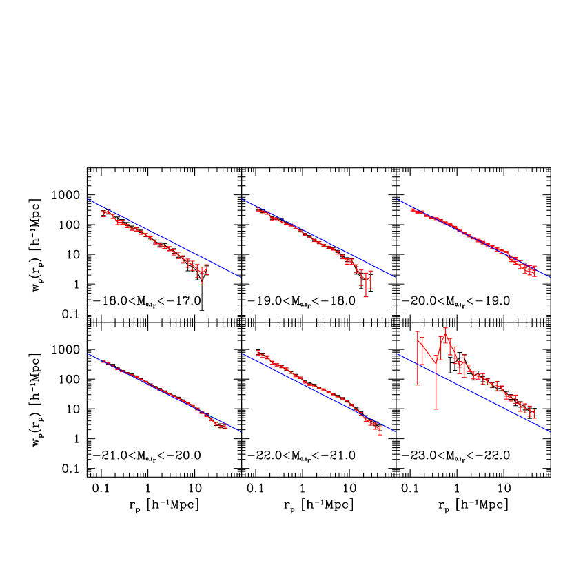
Fig.3 shows the projected 2PCF $w_{p}(r_{p})$ in different luminosity intervals (Samples L3, L5, L7, L9, L11 and L13 in Table 1). The red and black lines on the figure compare the results obtained for the two different methods of constructing random samples described in Section 3.1. Black lines are for the “standard” method in which the selection function is explicitly modelled. Red lines are for the method in which the sky positions of the observed galaxies are randomly re-assigned. The agreement between the two methods is very encouraging, suggesting that the latter method does work well for analyzing large redshift surveys like the SDSS and can be applied in the case of more complicated selection by physical parameters with redshift-dependent biases.

To guide the eye, we have plotted the relation $\xi(r)=(r/5h^{-1}\mbox{Mpc})^{-1.8}$ in blue in every panel in Fig.3. In general, we see that the amplitude of the correlation function increases with luminosity, but the strength of this effect is different on different scales. For galaxies fainter than $L^{\ast}$ ($M_{{}^{0.1}r}=-20.44$), the clustering amplitude stays nearly constant on very small scales ($r_{p}\sim 0.1\>h^{-1}{\rm{Mpc}}$), but on larger scales there is a much stronger luminosity dependence. For bright galaxies, the correlation amplitude increases strongly with luminosity at all scales. It is also interesting that the slope of the correlation function gets flatter with increasing luminosity for galaxies fainter than $L^{\ast}$, but then increases for galaxies brighter than $L^{\ast}$. In another word, $L^{\ast}$ galaxies exhibit the flattest correlation functions.

These trends are illustrated more clearly in Fig.4, where we plot the amplitude of the projected correlation function $w_{p}(r_{p})$ as a function of luminosity at $r_{p}=$0.2, 1, 5, and 10$\>h^{-1}{\rm{Mpc}}$. At $r_{p}$= 0.2 $\>h^{-1}{\rm{Mpc}}$, the correlation function probes galaxy pairs that reside within a common dark matter halo. At $r_{p}$ = 10 $\>h^{-1}{\rm{Mpc}}$ the correlation function should only be sensitive to pairs of galaxies in separate haloes. This figure confirms that luminous galaxies cluster more strongly than faint galaxies, with the difference becoming more marked above $L^{\ast}$. However, the luminosity dependence of galaxy clustering is different on different scales. On small scales, the clustering amplitude does not vary with luminosity for galaxies fainter than $L^{\ast}$, but increases steeply for galaxies brighter than $L^{\ast}$. In contrast, the amplitude on large scales rises more continuously as a function of luminosity. It is also interesting that the dependence of $w_{p}(r_{p})$ on luminosity appears to change slope at $M_{{}^{0.1}r}\sim-20$. One possible reason for this switch in behaviour is that a significant fraction of faint galaxies are “satellite” systems orbiting within a common dark matter halo, whereas bright galaxies are mainly “central” galaxies located at the centers of their dark matter haloes. We intend to explore this in more detail in future work.

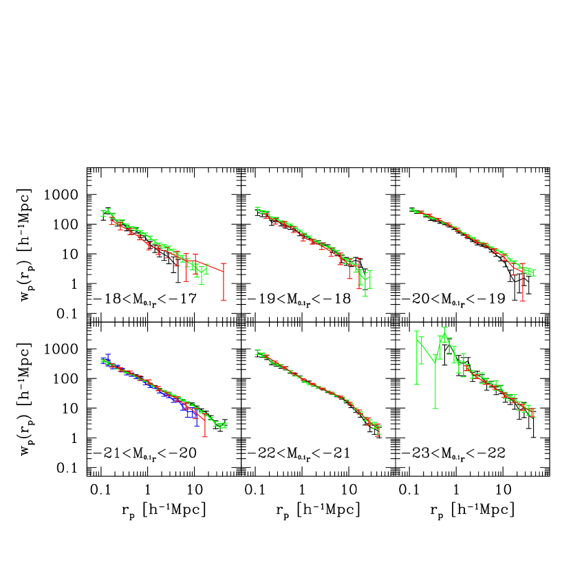
To compare our results to previous studies, we have also computed correlation functions using samples that are volume-limited in luminosity (Samples VL1-VL7). The results are shown in Fig.5. Black lines show the correlation functions for samples VL1-VL7. For comparison, the measurements provided by Z05 are shown in red and the correlation functions computed from the corresponding magnitude-limited subsamples are shown in green. The agreement between the magnitude-limited analysis and the volume-limited one indicates that our results are robust and reliable. Furthermore, it can be seen that our measurements are in good agreement with those carried out by Z05, although there are some small differences. These are probably due to the different 2PCF estimators or the different methods of constructing random samples. We note that the magnitude-limited sample of galaxies with $-20<M_{{}^{0.1}r}<-19$ (Sample L7) and the magnitude-limited and volume-limited samples with $-21<M_{{}^{0.1}r}<-20$ (Sample L9 and VL5) all exhibit anomalously high $w_{p}(r_{p})$ values at large separations ($r_{p}\lower 2.15277pt\hbox{$\;\buildrel>\over{\sim}\;$}5\>h^{-1}{\rm{Mpc}}$). As pointed out by Z05, this anomalous behavior is a “cosmic variance” effect caused by an enormous supercluster at $z\sim 0.08$, which overlaps these three samples. When the Sample VL5 is restricted to redshifts below 0.07, its projected correlation functions drops and steepens, (blue line in Fig.5), coming into good agreement with that of Z05.

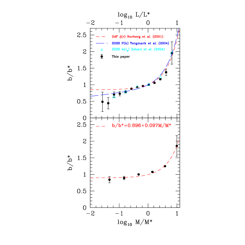
Following Z05, we calculate the relative bias factor $b/b^{\ast}$ as a function of normalized luminosity $L/L^{\ast}$. The relative bias factor is defined by the amplitude of $w_{p}(r_{p})$ measured at a fixed separation $r_{p}=2.7h^{-1}$ Mpc relative to the value measured for the $-21<M_{{}^{0.1}r}<-20$ subsample (Sample L9, which has $L\approx L^{\ast}$). This fiducial separation of $2.7h^{-1}$ Mpc was chosen because it is well out of the very non-linear regime, but still small enough so that the correlation functions are very accurately measured in all surveys. The solid circles in Fig.6 show our results and the triangles show the SDSS results from Z05. The long dashed curve is taken from Tegmark et al. (2004), where bias factors are derived from the galaxy power spectrum $P(k)$ at wavelength $2\pi/k\sim 100\>h^{-1}{\rm{Mpc}}$. The results in this paper and in Z05, both of which are derived from $w_{p}(r_{p})$ measurements, agree very well (as they should). Our results are also in quite good agreement with those of Tegmark et al. The dashed curve in Fig.6 shows the result of Norberg et al. (2001), based on $w_{p}(r_{p})$ measurements of somewhat more luminous galaxies in the 2dF survey ($\log_{10}L/L^{\ast}\lower 2.15277pt\hbox{$\;\buildrel>\over{\sim}\;$}-0.6$). The agreement is again very good over the range of luminosities where the different analyses overlap.

Figure 7: Projected 2PCF for stellar mass subsamples, as indicated. The red lines are for the results obtained by applying volume corrections, compared with those without applying the corrections (black). The blue lines in some panels are for the samples that are volume-limited in $M_{\ast}$. In each panel, the green line is the line corresponding to $\xi(r)=(r/5h^{-1}\mbox{Mpc})^{-1.8}$.

Figure 8: Examples of the bimodal distribution of physical quantities in different luminosity intervals, as indicated. In each panel, the histogram is for the data, whileas the green and blue lines are the best fit Gaussians and the red is the total. $N_{0}$ is the maximum of the total fit, and the quantities with a zero give the median of the two Gaussian centers.

Figure 9: Contours of number density of galaxies in the planes of luminosity vs physical quantities. The black lines are for the data, whileas the red are reconstructed according to the best-fitting bi-Gaussians (see Fig.8; also see the text for a detailed description). The blue lines are the best linear fits to the median Gaussian centers as a function of luminosity (see Fig.8). These are the luminosity-dependent cuts that we adopt for dividing galaxies according to a given physical property. The green line in the top-left panel is the $g-r$ cut adopted by Zehavi et al. (2005).

4.2 Stellar mass

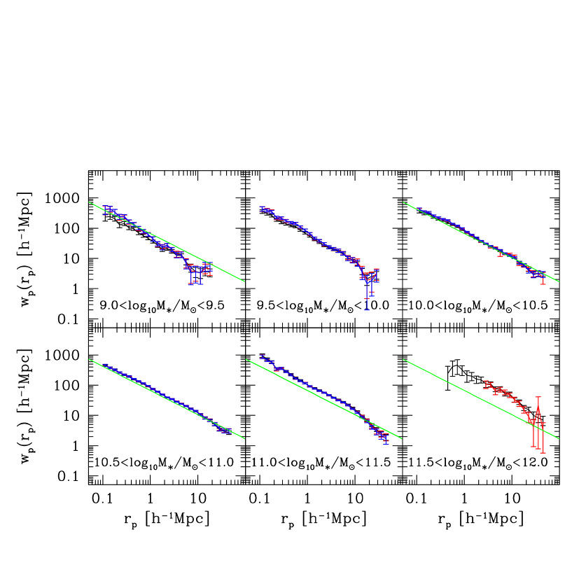
In this section, we present measurements of the projected 2PCF $w_{p}(r_{p})$ as a function of stellar mass. As discussed in section 3.2, when computing $w_{p}(r_{p})$ as a function of mass, we weight each galaxy pair by the inverse of the volume over which both galaxies can be detected in the survey. The effect of this correction can be seen in Fig.7 by comparing the black lines (no volume-weighting) with the red lines (with volume-weighting). As can be seen, the volume correction steepens the correlation function of low mass galaxies. Recall that if no volume correction is applied, the sample is biased towards galaxies with low $M_{\ast}/L$ ratios. As we will show in detail in the following section, the slope of the correlation function is very sensitive to the colour (and hence the young stellar content) of galaxies, particularly for low mass systems. This is why the volume corrections make the most difference for galaxies in our two lowest mass bins. We have also compared our results with the measurements obtained using samples that are volume-limited in stellar mass (blue lines). As can be seen, the results obtained for the volume-limited samples agree very well with the volume-corrected $w_{p}(r_{p})$.

The bottom panel of Fig.6 shows the relative bias factor $b/b^{\ast}$ at $r_{p}=2.7\>h^{-1}{\rm{Mpc}}$ as a function of stellar mass, with points showing the results from our $w_{p}(r_{p})$ measurements based on samples M1-M6, and dashed lines showing the fit to the measurements $b/b^{\ast}=0.90+0.10M/M^{\ast}$. The value $M^{\ast}$ is determined by fitting a Schechter function to the stellar mass function of the galaxies in our sample. We obtain $M^{\ast}=(4.11\pm 0.02)\times 10^{10}h^{-2}M_{\odot}$, $\alpha=-1.073\pm 0.003$ and $\phi^{\ast}=0.0204\pm 0.0001h^{3}$Mpc^-3 (Wang et al. , in preparation). Qualitatively, the behaviour of the relative bias as a function of $M_{\ast}$ is very similar to the results obtained as a function of $L$. This is not surprising, because luminosity and stellar mass are reasonably tightly correlated (see Fig. 2). What is of interest, however, is that these measurements can be used to set constraints on the fraction of baryons that have been turned into stars in dark matter haloes of different mass. We will come back to this in future work.

4.3 Division by physical parameters

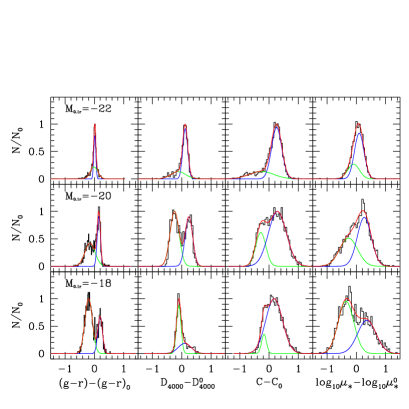
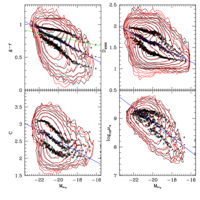
We now investigate how the clustering of galaxies of given luminosity (or stellar mass) depends on properties such as colour, 4000 Å break strength, concentration and surface mass density. Z05 performed such an analysis in the space of luminosity vs $g-r$ colour. They adopted a tilted colour cut motivated by the colour-magnitude diagram. A similar colour division is presented in Baldry et al. (2004), who found that the distribution of galaxy colour could be well approximate using bi-Gaussian functions (see Baldry et al. 2004, also see Fig.8 here). Fig.8 shows that other physical quantities, such as D₄₀₀₀, $C$ and $\mu_{\ast}$ also exhibit bimodal distributions. We thus fit bi-Gaussian functions to the distribution of $g-r$, D₄₀₀₀, $C$ and $\log\mu_{\ast}$ for each of the 282 luminosity subsamples described in §3.1. These are shown in Fig.8 for three representative luminosity intervals. In Fig.9 we illustrate how well these fits recover the true distribution of these parameters as a function of luminosity. Black lines show contours of the actual number density of galaxies and red lines show the predicted number densities from the bi-Gaussian fits. As can be seen, the bi-Gaussian model does a reasonable job of reproducing the observations.

Table 4: Coefficients for the formula of dividers in physical quantities

Quantity	A	B
$g-r$	-0.788 $\pm$ 0.028	-0.078 $\pm$ 0.001
D4000	-0.563 $\pm$ 0.038	-0.108 $\pm$ 0.002
$C$	-0.498 $\pm$ 0.193	-0.150 $\pm$ 0.009
$\log_{10}\mu_{\ast}$	3.738$\pm$0.213	-0.256 $\pm$0.011

The division of the luminosity subsamples into red and blue, high D₄₀₀₀ and low D₄₀₀₀, high concentration and low concentration, high surface density and low surface density, is defined as the mean of the two Gaussian centers in each luminosity bin. In Fig. 9, triangles indicate the two Gaussian centers and the crosses are the mean of these centers. We fit the dividing point as a function of luminosity using a linear equation of the form (see Fig.9, blue lines),

$$P=A+B\cdot M_{{}^{0.1}r},$$ (7)

where $P$ is the physical parameter under investigation, and $A$ and $B$ are the best-fitting linear coefficients. These are listed in Table 4 for reference. Using these best-fitting cuts (Eqn.7), we divide the galaxies in each of the 13 luminosity samples (Sample L1-L13) and the 5 stellar mass samples (M1-M5) into two further subsamples. For simplicity, we use “red” to denote the subsamples with larger values of the physical quantity and “blue” for the subsamples with the smaller value. The percentage of galaxies in the “red” subsamples are listed in the last 4 columns of Table 1.

Figure 10: Projected correlation function $w_{p}(r_{p})$ for galaxies in different luminosity intervals and with different properties (from left to right: $g-r$ colour, D₄₀₀₀, concentration and $\log$ stellar surface mass density $\log_{10}\mu^{\ast}$). The panels in each colume are for different luminosity subsamples, with the range of absolute magnitude indicated in the left column. In each panel, the black is for the full sample, the red (blue) is for the subsample with larger(smaller) value of the corresponding physical parameter. In each panel, the green line is the line corresponding to $\xi(r)=(r/5h^{-1}\mbox{Mpc})^{-1.8}$.

Figure 11: $w_{p}(r_{p})$ measured at $r_{p}=0.2,1,5,$ and $10\>h^{-1}{\rm{Mpc}}$, as a function of luminosity. The different columns show the dependence on different physical quantities, as indicated. In each panel, the black is for the full sample, the red (blue) is for the subsample with larger(smaller) value of the corresponding physical parameter.

Figure 12: Projected correlation function $w_{p}(r_{p})$ for galaxies in different stellar mass intervals and with different physical properties (from left to right: $g-r$ colour, D₄₀₀₀, concentration and $\log$ stellar surface mass density $\log_{10}\mu^{\ast}$). The panels in each column are for different stellar mass subsamples, with the range of stellar mass indicated in the left column. In each panel, the black is for the full sample, the red (blue) is for the subsample with larger(smaller) value of the corresponding physical parameter, and the green line is the line corresponding to $\xi(r)=(r/5h^{-1}\mbox{Mpc})^{-1.8}$.

Figure 13: $w_{p}(r_{p})$ measured at $r_{p}=0.2,1,5,$ and $10\>h^{-1}{\rm{Mpc}}$, as a function of stellar mass. The different columns show the dependence on different physical quantities, as indicated. In each panel, the black is for the full sample, the red (blue) is for the subsample with larger(smaller) value of the corresponding physical parameter.

Figure 14: Projected correlation functions measured at $r_{p}=0.2,1,5$ and $10h^{-1}$ Mpc, as a function of different physical parameters. In all panels, the stellar mass are limited to the range $10<\log_{10}M_{\ast}/M_{\odot}<11$.

4.3.1 In luminosity bins

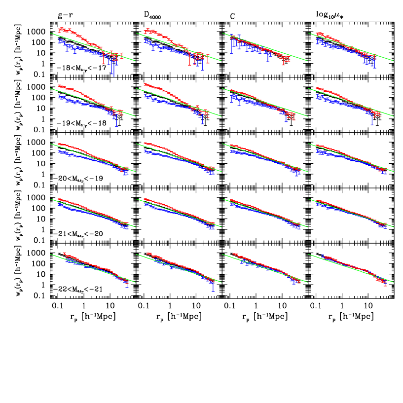
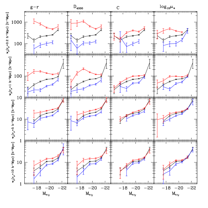
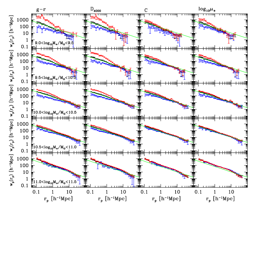
The projected 2PCFs in the space of luminosity vs colour, D₄₀₀₀, concentration and surface density are presented in Fig.10. Red (blue) lines correspond to the “red” (“blue”) subsamples. Black lines are for the sample as a whole. Fig. 11 shows the measurements of the amplitude of $w_{p}(r_{p})$ at $r_{p}=$ 0.2, 1, 5 and 10 $\>h^{-1}{\rm{Mpc}}$.

When the sample is divided by $g-r$ colour, redder galaxies of all luminosities are more strongly clustered and have steeper correlation functions than their blue counterparts. This colour dependence is much stronger for faint galaxies than for bright galaxies, particularly on small scales. Fig. 11 shows that the clustering amplitude of blue galaxies increases as a function of luminosity at all scales. However, the situation is more complicated for red galaxies. On small scales, faint red galaxies are clustered more strongly than bright red galaxies. On large scales, however, the trend reverses and the clustering amplitude increases with luminosity. These results are all consistent with the findings of Z05. The behaviour of the slope of the correlation function as a function of luminosity is also different for red and blue galaxies. The correlation function of faint red galaxies is very steep and the slope flattens systematically as luminosity increases. In contrast, the slope of the correlation function of blue galaxies exhibits rather little change with luminosity. All these trends are qualitatively consistent with a picture in which faint red galaxies are primarily “satellite” systems in massive dark matter haloes, but faint blue galaxies occupy haloes of smaller mass (Z05; Berlind et al. 2005; Li et al. 2006).

Our results show that the dependence of clustering on D₄₀₀₀ is very similar to what is obtained for $g-r$ colour. On the other hand, rather different results are obtained for the structural parameters $C$ and $\mu_{\ast}$. Fig. 11 clearly shows that the dependence of $w_{p}(r_{p})$ on $g-r$/D₄₀₀₀ is considerably stronger than the dependence on $C$/$\mu_{\ast}$ at all physical scales.

4.3.2 In stellar mass bins

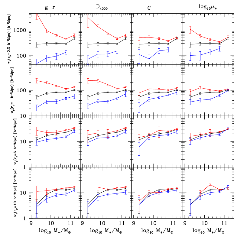
The projected 2PCFs in the space of stellar mass vs the same set of physical parameters are presented in Fig.12. The measurements at $r_{p}=$ 0.2, 1, 5 and 10$\>h^{-1}{\rm{Mpc}}$ are plotted in Fig.13.

Qualitatively, the results shown in Figs. 11 and 13 appear very similar. However, careful comparison of these two figures shows that interesting quantitative differences do exist between the clustering of the “red” and “blue” subsamples at fixed luminosity and at fixed stellar mass. On small scales, the dependences are stronger when evaluated at fixed mass, particularly for low mass galaxies. We also note that there is a small difference in the clustering amplitude of the “red” and “blue” subsamples at projected radii as large as 10 $h^{-1}$ Mpc in Fig. 11. This difference is seen both in $g-r$ colour and D₄₀₀₀ and more weakly in the structural parameters $C$ and $\mu_{\ast}$. Fig. 13 shows, however, that at fixed stellar mass there is no longer any significant difference in the clustering amplitude of high concentration and low concentration galaxies or high surface density and low surface density galaxies on scales larger than 5 $h^{-1}$ Mpc. The clustering differences in $g-r$ and D₄₀₀₀ do persist, however. This is a rather surprising result, because at scales larger than a few Mpc, galaxies inside the same dark matter halo no longer contribute to the clustering signal. Our result thus indicates that at fixed stellar mass, the clustering properties of the surrounding dark matter haloes are somehow correlated with the colour of the selected galaxies.

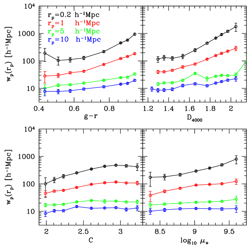
To investigate this effect further, we have computed the 2PCF as a function of $g-r$, D₄₀₀₀, $C$ and $\mu_{\ast}$ for galaxies spanning a narrow range in stellar mass ($10^{10}-10^{11}M_{\odot}$). In Fig.14, we plot the amplitude of the correlation function as a function of these quantities measured on four different physical scales ($r_{p}$= 0.2,1, 5 and 10$\>h^{-1}{\rm{Mpc}}$). This figure confirms that the dependence of $w_{p}(r_{p})$ on $g-r$/D₄₀₀₀ extends out to larger physical scales than the dependence of $w_{p}(r_{p})$ on $C$/$\mu_{\ast}$. The figure also shows that the dependence of $w_{p}(r_{p})$ on $C$ and $\mu_{\ast}$ is also qualitatively quite different on small scales. On scales less than $<1h^{-1}$ Mpc, the amplitude of the correlation function is constant for “young” galaxies with $1.1<$D${}_{4000}<1.5$ and a steeply rising function of age for “older” galaxies with D${}_{4000}>1.5$. In contrast, the dependence of the amplitude of $w_{p}(r_{p})$ on concentration is strongest for disk-dominated galaxies with $C<2.6$ on these same scales. This demonstrates that different physical processes are required to explain environmental trends in star formation and in galaxy structure.

5 Summary and Discussion

In this paper we present our determinations of the projected two-point correlation function (2PCF) $w_{p}(r_{p})$ for different classes of galaxies in order to study the dependence of clustering on the physical properties of these systems. We use the New York University Value Added Catalog (NYU-VAGC) which is constructed from the the Sloan Digital Sky Survey Data Release Two (SDSS DR2).

The conclusions of this paper can be summarized as follows:

1. We confirm previous findings that luminous galaxies cluster more strongly than faint galaxies, with the difference becoming larger for galaxies with $L>L^{\ast}$, where $L^{\ast}$ is the characteristic luminosity of the Schechter (1976) function. The dependence of galaxy clustering on luminosity is different on different physical scales. On small scales ($r_{p}\sim 0.2\>h^{-1}{\rm{Mpc}}$), the correlation amplitude is almost constant for galaxies fainter than $L^{\ast}$, but the amplitude increases sharply above $L^{\ast}$. On large scales, the correlation amplitude increases more continuously as a function of luminosity. Around $L^{\ast}$ there appears to be a shoulder, with $w_{p}(r_{p})$ increasing more steeply with $L$ for higher-luminosity galaxies. Our results are in good agreement with previous studies of clustering as a function of luminosity in the SDSS.

2. We present $w_{p}(r_{p})$ as a function of stellar mass. In analogy with previous results obtained as a function of luminosity, we find that more massive galaxies cluster more strongly than less massive galaxies, with the difference increasing above the characteristic stellar mass $M^{\ast}$ of the Schechter mass function.

3. When galaxies are divided according to their physical properties, we find that galaxies with redder colours, larger 4000Å break strengths, more concentrated structure, and higher surface mass densities cluster more strongly and have steeper correlation functions at all luminosities and masses. The differences in clustering strength are larger on small scales and for low-luminosity and less massive galaxies.

4. We have found that the dependence of $w_{p}(r_{p})$ on $g-r$ or D₄₀₀₀ extends out to larger physical scales ($r_{p}>5\>h^{-1}{\rm{Mpc}}$) than the dependence of $w_{p}(r_{p})$ on $C$ or $\mu_{\ast}$. On small scales ($\sim 0.2\>h^{-1}{\rm{Mpc}}$), the behaviour of $w_{p}(r_{p})$ as a function of $g-r$ or D₄₀₀₀ and as a function of $C$ are qualitatively different.

We have chosen not to express our results in terms of power-law fits to our $w_{p}(r_{p})$ measurements. We have tabulated the measurements of our correlation functions so that they can be accurately recovered. As discussed by Z05, a single power-law is a poor description of the data and as we expand our exploration of physical parameter space, it is important not to place unnecessary restrictions on the way in which the observational results are described. In this paper, we have chosen to plot trends in clustering amplitude evaluated on a variety different physical scales. This leads to a number of interesting insights that have not received much attention up to now : (1) the dependence of the clustering amplitude (or equivalently, the relative bias factor) on luminosity is qualitatively different on small scales and on large scales, (2) there is a different scale dependence in the amplitude of the correlation function for parameters that measure the star formation histories of galaxies and for parameters that measure galaxy structure, suggesting that the trends in star formation and in galaxy structure are governed by different physical processes.

Finally, it is worth comparing our results with the many studies that have examined correlations between galaxy properties and the local environment. One of the most fundamental correlations between the properties of galaxies in the local Universe is the so-called morphology-density relation. Oemler (1974) and Dressler (1980) pioneered the quantification of this relation, showing that spheroidal systems reside preferentially in dense regions. Since the standard morphological classification scheme mixes elements that depend on the structure of a galaxy with elements related to its recent star formation history, it is by no means obvious that these two elements should depend on environment in the same way.

Recent studies using large surveys such as the SDSS have revealed that galaxy colour is the galaxy property most predictive of the local environment (e.g. Blanton et al. 2005b; Kauffmann et al. 2004). Hogg et al. (2003) show that the local density increases strongly with luminosity for the brightest galaxies. For faint galaxies, local density is senstive mainly to color, with faint red galaxies occupying highest-density regions. Blanton et al. (2005b) found that at fixed luminosity and colour, density is not closely related to surface brightness or to the S$\acute{e}$rsic index (a quantity related to galaxy structure), so that morphological properties of galaxies are less closely related to galaxy environment than their luminosities and star formation histories. Kauffmann et al. (2004) obtained very similar results. They found that at fixed stellar mass both star formation and nuclear activity depend strongly on local density, while structural parameters such as size and concentration are almost independent of it.

Our analyses of $w_{p}(r_{p})$ as a function of luminosity, colour and structural parameters are consistent with these conclusions. The power of the $w_{p}(r_{p})$ statistic is that it encapsulates information about how galaxy properties depend on environment over a wide range of physical scales. Kauffmann et al. (2004) found no evidence for a significant dependence of galaxy structure on local density. However, their local densities are calculated in a fixed aperture of 2 $\>h^{-1}{\rm{Mpc}}$, whereas our plots (see Fig.14) show clearly that the dependence of structural parameters on environment becomes significant on scales that are smaller than this value.

The other advantage of $w_{p}(r_{p})$ is that it is can be very easily compared with the predictions of galaxy formation simulations. It probes the physical processes occurring inside individual dark matter haloes as well the masses of the dark matter haloes that host galaxies of given mass, luminosity, size, age and concentration, thus placing strong constraints on theoretical models. This will be the focus of future work.

Appendix A Description of Online Tables

Tables 5 and 6 contain our $w_{p}(r_{p})$ measurements for the galaxies with different luminosities/stellar masses. Results are also given as a function of the physical quantities $g-r$, D₄₀₀₀, $C$ and $\mu_{*}$. The tables are available in electronic form at http://www.mpa-garching.mpg.de/^∼leech/papers/clustering/.

Tables 5 and 6 list the data points in Figs.10 and 12 respectively, i.e. the measured projected 2PCF $w_{p}(r_{p})$ for galaxies in different luminosity or stellar mass intervals and with different properties. Table 5 consists of 13 separate parts corresponding to the 13 luminosity samples (Samples L1-L13 in Table 1). Likewise, Table 6 consists of 5 parts corresponding to the 5 stellar mass samples (Samples M1-M5 in Table 1). To make the description clearer, we present here an abridged version for the first part in Table 5, listing only the first several rows for Sample L1. The first column is the projected separation $r_{p}$ in unit of $\>h^{-1}{\rm{Mpc}}$, ranging from $\sim 0.1\>h^{-1}{\rm{Mpc}}$ up to $\sim 45\>h^{-1}{\rm{Mpc}}$. The other columns give the $w_{p}(r_{p})$ measurements and errors for the full luminosity/stellar mass sample (Column 2) and the ”red” and ”blue” subsamples divided by $g-r$ (Columns 3-4), D₄₀₀₀ (Columns 5-6), $C$ (Columns 7-8) and $\log_{10}\mu_{\ast}$ (Columns 9-10). Short straight lines denote the points that have no measurements, either because of low S/N or for any other reason.

References

- [Abazajian et al. (2004)] Abazajian, K., et al. 2004, AJ, 128, 502
- [\citeauthoryearBaldry et al.2004] Baldry I. K., Glazebrook K., Brinkmann J., Ivezić Ž., Lupton R. H., Nichol R. C., Szalay A. S., 2004, ApJ, 600, 681
- [\citeauthoryearBalogh et al. 1999] Balogh M. L., Morris S. L., Yee H. K. C., Carlberg R. G., Ellingson E., 1999, ApJ, 527, 54
- [Barrow, Bhavsar, & Sonoda(1984)] Barrow, J. D., Bhavsar, S. P., & Sonoda, D. H. 1984, MNRAS, 210, 19
- [\citeauthoryearBenson et al. 2000b] Benson A. J., Baugh C. M., Cole S., Frenk C. S., Lacey C. G., 2000b, MNRAS, 316, 107
- [\citeauthoryearBenson et al. 2000a] Benson A. J., Cole S., Frenk C. S., Baugh C. M., Lacey C. G., 2000a, MNRAS, 311, 793
- [\citeauthoryearBerlind & Weinberg2002] Berlind A. A., Weinberg D. H., 2002, ApJ, 575, 587
- [\citeauthoryearBerlind et al.2005] Berlind A. A., Blanton M. R., Hogg D. W., Weinberg D. H., Davé R., Eisenstein D. J., Katz N., 2005, ApJ, 629, 625
- [Blanton et al. (2003a)] Blanton, M. R., Brinkmann, J., Csabai, I., Doi, M., Eisenstein, D. J., Fukugita, M., Gunn, J. E., Hogg, D. W. & Schlegel, D. J. 2003a, AJ, 125, 2348
- [Blanton et al. (2003b)] Blanton, M. R., Lin, H., Lupton, R. H., Maley, F. M., Young, N., Zehavi, I., & Loveday, J. 2003b, AJ, 125, 2276
- [Blanton et al. (2003c)] Blanton, M. R., Lin, H., Lupton, R. H., Maley, F. M., Young, N., Zehavi, I., & Loveday, J. 2003c, ApJ, 592, 819
- [\citeauthoryearBlanton et al. 2005a] Blanton M. R., et al. , 2005a, AJ, 129, 2562
- [\citeauthoryearBlanton et al. 2005b] Blanton M. R., Eisenstein D., Hogg D. W., Schlegel D. J., Brinkmann J., 2005b, ApJ, 629, 143
- [\citeauthoryearBrinchmann et al. 2004] Brinchmann J., Charlot S., White S. D. M., Tremonti C., Kauffmann G., Heckman T., Brinkmann J., 2004, MNRAS, 351, 1151
- [\citeauthoryearBruzual & Charlot2003] Bruzual G., Charlot S., 2003, MNRAS, 344, 1000
- [\citeauthoryearBudavári et al. 2003] Budavári T., et al. , 2003, ApJ, 595, 59
- [\citeauthoryearCooray & Sheth2002] Cooray A., Sheth R., 2002, PhR, 372, 1
- [\citeauthoryearDavis & Geller1976] Davis M., Geller M. J., 1976, ApJ, 208, 13
- [Dressler(1980)] Dressler, A. 1980, ApJ, 236, 351
- [\citeauthoryearFukugita et al. 1996] Fukugita M., Ichikawa T., Gunn J. E., Doi M., Shimasaku K., Schneider D. P., 1996, AJ, 111, 1748
- [Goto et al. (2003)] Goto T., Yamaguchi C., Fujita Y., Okamura S., Sekiguchi M., Smail I., Bernardi M., Gomez P., 2003, MNRAS, 346, 601
- [\citeauthoryearGross et al. 1998] Gross M. A. K., Somerville R. S., Primack J. R., Holtzman J., Klypin A., 1998, MNRAS, 301, 81
- [\citeauthoryearGunn et al. 1998] Gunn J. E., et al. , 1998, AJ, 116, 3040
- [Hamilton(1993)] Hamilton, A. J. S. 1993, ApJ, 417, 19
- [Hamilton & Tegmark(2002)] Hamilton, A. J. S. & Tegmark, M. 2002, MNRAS, 330, 506
- [Hawkins et al. (2003)] Hawkins, E., et al. 2003, MNRAS, 346, 78
- [\citeauthoryearHogg et al. 2001] Hogg D. W., Finkbeiner D. P., Schlegel D. J., Gunn J. E., 2001, AJ, 122, 2129
- [\citeauthoryearHogg et al.2003] Hogg D. W., et al., 2003, ApJ, 585, L5
- [\citeauthoryearIvezić et al. 2004] Ivezić Ž., et al. , 2004, AN, 325, 583
- [\citeauthoryearJenkins et al. 1998] Jenkins A., et al. , 1998, ApJ, 499, 20
- [Jing & Börner(2004)] Jing, Y. P. & Börner, G. 2004, ApJ, 617, 782
- [Jing, Mo, & Börner(1998)] Jing, Y. P., Mo, H. J. & Börner, G. 1998, ApJ, 494, 1
- [\citeauthoryearKauffmann, Nusser, & Steinmetz1997] Kauffmann G., Nusser A., Steinmetz M., 1997, MNRAS, 286, 795
- [\citeauthoryearKauffmann et al. 1999] Kauffmann G., Colberg J. M., Diaferio A., White S. D. M., 1999, MNRAS, 303, 188
- [\citeauthoryearKauffmann et al. 2003a] Kauffmann G., et al. , 2003a, MNRAS, 341, 33
- [\citeauthoryearKauffmann et al. 2003b] Kauffmann G., et al. , 2003b, MNRAS, 341, 54
- [Kauffmann et al. (2004)] Kauffmann, G., et al. 2004, MNRAS, 353, 713
- [\citeauthoryearLi et al.2006] Li C., Jing Y. P., Kauffmann G., Boerner G., White S. D. M., Cheng F. Z., 2006, MNRAS, 368, 37
- [\citeauthoryearMadgwick et al. 2003] Madgwick D. S., et al. , 2003, MNRAS, 344, 847
- [Miller et al. (2003)] Miller C. J., Nichol R. C., Gomez P. L., Hopkins A. M., Bernardi M., 2003, ApJ, 597, 142
- [Mo, Jing, & Börner(1992)] Mo, H. J., Jing, Y. P., Börner, G. 1992, ApJ, 392, 452
- [Norberg et al. (2001)] Norberg, P., et al. 2001, MNRAS, 328, 64
- [Norberg et al. (2002)] Norberg, P., et al. 2002, MNRAS, 332, 827
- [Oemler(1974)] Oemler, A. 1974, ApJ, 194, 1
- [\citeauthoryearPeacock & Smith2000] Peacock J. A., Smith R. E., 2000, MNRAS, 318, 1144
- [Peebles(1980)] Peebles, P.J.E. 1980, The Large-Scale Structure of the Universe, Princeton University Press, Princeton
- [\citeauthoryearPier et al. 2003] Pier J. R., Munn J. A., Hindsley R. B., Hennessy G. S., Kent S. M., Lupton R. H., Ivezić Ž., 2003, AJ, 125, 1559
- [\citeauthoryearSchechter1976] Schechter P., 1976, ApJ, 203, 297
- [Schlegel, Finkbeiner, & Davis(1998)] Schlegel, D. J., Finkbeiner, D. P, & Davis, M. 1998, ApJ, 500, 525
- [\citeauthoryearSeljak2000] Seljak U., 2000, MNRAS, 318, 203
- [\citeauthoryearSmith et al. 2002] Smith J. A., et al. , 2002, AJ, 123, 2121
- [\citeauthoryearStoughton et al. 2002] Stoughton C., et al. , 2002, AJ, 123, 485
- [\citeauthoryearStrateva et al. 2001] Strateva I., et al. , 2001, AJ, 122, 1861
- [Tegmark, Hamilton & Xu(2002)] Tegmark, M., Hamilton, A. J. S., & Xu,Y. 2002, MNRAS, 335, 887
- [Tegmark et al. (2004)] Tegmark, M., et al. 2004, ApJ, 606, 702
- [\citeauthoryearWorthey & Ottaviani1997] Worthey G., Ottaviani D. L., 1997, ApJS, 111, 377
- [\citeauthoryearYang, Mo, & van den Bosch2003] Yang X., Mo H. J., van den Bosch F. C., 2003, MNRAS, 339, 1057
- [York et al. (2000)] York, D. G., et al. 2000, AJ, 120, 1579
- [Zehavi et al. (2002)] Zehavi, I., et al. 2002, ApJ, 571, 172
- [Zehavi et al. (2004)] Zehavi, I., et al. 2004, ApJ, 608, 16
- [\citeauthoryearZehavi et al.2005] Zehavi I., et al., 2005, ApJ, 630, 1