Conservation of nonlinear curvature perturbations on super-Hubble scales

Abstract

We consider general, non-linear curvature perturbations on scales greater than the Hubble horizon scale by invoking an expansion in spatial gradients, the so-called gradient expansion. After reviewing the basic properties of the gradient expansion, we derive the conservation law for non-linear curvature perturbations for an isentropic fluid. We also define the gauge-invariant curvature perturbation under a finite shift of time-slicing, and derive the non-linear genralization of the $\delta N$ formalism. The results obtained are straight-forward generalisations of those already proven in linear perturbation theory, and the equations are simple, resembling closely the first-order equations.

1 Introduction

Analysis of the WMAP first-year data Bennett:2003bz revealed that the standard inflationary universe scenario in which a single inflaton field slowly rolls down its potential hill during inflation is perfectly consistent with the observed CMB temperature spectrum Hinshaw:2003ex . Namely, the CMB anisotropy theoretically predicted from a scale-invariant adiabatic perturbation in a spatiall flat universe matched with the observed CMB anisotropy with impressive precision Spergel:2003cb , and no non-Gaussianity was found in the statistics of the observed anisotropy Komatsu:2003fd . This not only means the validity of the standard inflationary theory but also justifies the use of linear cosmological perturbation theory Bardeen80 ; KodSas ; Mukhanov .

Nevertheless, there are some features in the observed CMB spectrum which might not be caused simply by cosmic variance but that could be a signature of non-standard inflation such as multi-field inflation, non-slow-roll inflation, braneworld inflation, etc.. Also, the level of the Gaussianity test is still not stringent enough that there could be some non-Gaussianity which are to be found in future experiments, say, by PLANCK Planck . To deal with such cases properly, it is necessary to consider nonlinear perturbations on superhorizon scales.

Turning to the state of our present universe, the WMAP data also confirmed the existence of energy in the form of a cosmological constant or vacuum energy, now called the dark energy, and it dominates the energy density of the present universe. Because the energy scale of this vacuum (dark) energy is extremely small, of $O(10^{-3})$eV, compared to the Planck scale, $10^{19}$Gev, the confirmation of its existence was a big shock to theorists, especially those from the particle physics/string theory community.

Recently, several authors claimed that the present dark energy can be explained by backreaction of super-Hubble scale perturbations at second order Barausse:2005nf ; Kolb:2005me .

Nonlinear dynamics of cosmological perturbations on superhorizon scales has been discussed already by many authors gradient . But in the light of these new developments mentioned above, it is appropriate to revist the dynamics of cosmological perturbations on superhorizon scales, and clarify what can be said and what cannot be said.

In this report, we give a fully nonlinear formulation of cosmological perturbations on superhorizon scales at leading order in the gradient expansion, based on our recent paper LMS .

2 Gradient expansion

The gradient expansion is a powerful tool to deal with cosmological perturbations on superhorizon scales. It was developed by various authors for various purposes gradient . Here we first briefly describe the essence of it.

The gradient expansion assumes that spatial derivatives are always smaller than the time derivative for any physical quantity $Q$:

$$\left|\frac{\partial Q}{\partial x^{i}}\right|\ll\left|\frac{\partial Q}{\partial t}\right|.$$ (1)

In cosmological situations, we have $|\partial_{t}Q|\sim HQ$ where $H$ is the inverse of the Hubble timescale (or the gravitational free-fall timescale) and given by $H\sim\sqrt{8\pi G\rho/3}$. At each point of spacetime, we therefore have a local definition of the Hubble horizon size, given by $H^{-1}$. Hence the gradient expansion is valid if the quantities are slowly varying in space on the Hubble horizon scale.

At lowest order in the gradient expansion, the Einstein and matter field equations become ordinary differential equations in time. In other words, the evolution on scale of each Hubble size region, which we call ‘local’ evolution, should not depend on what is happening in some spatially distant part of the universe, as illustrated in Fig. 1. This is just a consequence of causality.

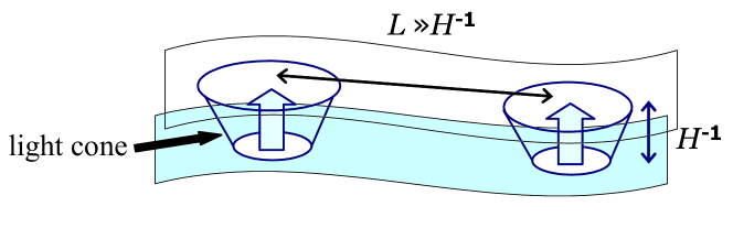
Figure 1: Schematic spacetime diagram for superhorizon scale cosmological perturbations. Each ‘local’ Hubble-horizon region evolves independently because of causality.

2.1 Metric

We consider the standard $(3+1)$-decomposition of the metric, which applies to any smooth spacetime:

$$ds^{2}=-{\cal{N}}^{2}dt^{2}+\gamma_{ij}(dx^{i}+\beta^{i}dt)(dx^{j}+\beta^{j}dt)\,,$$ (2)

where ${\cal{N}}$ is the lapse function, $\beta^{i}$ the shift vector, and $\gamma_{ij}$ the spatial three metric. (Greek indices will take the values $\mu,\nu=0,1,2,3$, Latin indices $i,j=1,2,3$. The spatial indices are to be raised or lowered by $\gamma^{ij}$ or $\gamma_{ij}$.) In this $(3+1)$-decomposition, the unit time-like vector normal to the $x^{0}=t=$const. hypersurface $n^{\mu}$ has the components,

$$n_{\mu}=\left[-{\cal{N}},0\right],\quad n^{\mu}=\left[\frac{1}{{\cal{N}}},-\frac{\beta^{i}}{{\cal{N}}}\right].$$ (3)

We write the 3-metric, $\gamma_{ij}$, as a product of two terms,

$$\gamma_{ij}\equiv e^{2\alpha}\tilde{\gamma}_{ij}\,,$$ (4)

where $\alpha$ and $\tilde{\gamma}_{ij}$ are functions of the spacetime coordinates $(t,x^{i})$, and $\det[\tilde{\gamma}_{ij}]=1$.

The above form of the metric is completely general. Now we apply it to the case of our interest, i.e., to cosmological situations in which the metric varies substantially on scales much greater than the Hubble horizon but is almost homogeneous and isotropic (and spatially flat) on scales of the Hubble horizon. Then, although it is not necessary, it is convenient to introduce a fiducial ‘background’ scale factor $a(t)$ and a perturbation $\psi$ on it as

$$e^{\alpha}=a(t)e^{\psi(t,x^{i})}\,.$$ (5)

Note that the variable $\psi$ describes the curvature perturbation in the limit of linear theory,

$${}^{(3)}R(\gamma)=-\frac{4}{a^{2}}{}^{(3)}\Delta\,\psi+O(\psi^{2})\,.$$ (6)

Hence we also call it the curvature perturbation, although there will be no simple relation between $\psi$ and ${}^{(3)}R$ in the nonlinear case.

Likewise, it is convenient to factorize the matrix $\tilde{\gamma}_{ij}$ as

$$\tilde{\gamma}\equiv Ie^{H}\,,$$ (7)

where $I$ is the unit matrix. The condition $\det(\tilde{\gamma})=1$ ensures that the matrix $H$ is traceless. In the limit of linear theory, the transverse part of $H_{ij}$ describes the tensor (gravitational wave) perturbation.

To invoke the gradient expansion, we associate an expansion parameter $\epsilon$ with each spatial derivative, $\partial_{i}\to\epsilon\partial_{i}$. Physically, $\epsilon$ is equal to the ratio of the Hubble horizon size to the typical wavelength of a perturbation, $\epsilon\sim H^{-1}/\lambda$. As for the form of the metric (2) is concerned, in order to apply the gradient expansion, the only non-trivial assumption we make is that

$$\beta^{i}=O(\epsilon)\,.$$ (8)

2.2 Matter

The energy-momentum tensor is assume to have the perfect fluid form

$$T_{\mu\nu}\equiv\left(\rho+P\right)u_{\mu}u_{\nu}+g_{\mu\nu}P\,,$$ (9)

where $\rho=\rho(x^{\mu})$ is the energy density and $P=P(x^{\mu})$ is the pressure. Then the energy conservation equation is

$$-u_{\mu}\nabla_{\nu}T^{\mu\nu}=\frac{d}{d\tau}\rho+\left(\rho+P\right)\theta=0\,,$$ (10)

where $d/d\tau=u^{\mu}\nabla_{\mu}$ and

$$\theta\equiv\nabla_{\mu}u^{\mu}\,.$$ (11)

In accordance with the assumption (8) on the shift vector $\beta^{i}$, we also assume that the 3-velocity of the matter to satisfy

$$v^{i}\equiv\frac{u^{i}}{u^{0}}=O(\epsilon)\,.$$ (12)

Then it follows that

$$\theta=\frac{3\partial_{t}\alpha}{{\cal{N}}}+O(\epsilon^{2})=\theta_{n}+O(\epsilon^{2})\,,$$ (13)

where

$$\theta_{n}\equiv\nabla_{\mu}n^{\mu}\,.$$ (14)

That is, the expansion of the matter 4-velocity and that of the unit vector normal to the hypersurface coincide to each other at lowest order in the gradient expansion, which follows from the assumptions (8) and (12).

One can then introduce the notion of the local Hubble parameter $\tilde{H}$ by

$$\tilde{H}\equiv\frac{1}{3}\theta=\frac{1}{3}\theta_{n}+O(\epsilon^{2})=\partial_{t}\alpha+O(\epsilon^{2})\,.$$ (15)

The second (or the last) equality implies that this defintion is unique in the sense that the local Hubble parameter can be defined in terms of the expansion of the hypersurface normal $n^{\mu}$, and the definition is independent of the choice of the time slicing. Here, we note again that ‘local’ means ‘on scales of the Hubble horizon size.’

2.3 Local Friedman equation

So far, we have not specified the theory of gravity. Let us now invoke Einstein gravity. By explicitly writing down the Einstein equations, one sees that one can further consistently assume LMS

$$\frac{\partial}{\partial t}\tilde{\gamma}_{ij}=O(\epsilon^{2})\,.$$ (16)

Physically this assumption means the absence of a decaying mode in the shear of the hypersurface. In the inflationary universe, this decaying mode dies out rapidly soon after the comoving scale of interest leaves out of the horizon. We then find that the only non-trivial equation is the $(0,0)$-component of the Einstein equations, i.e., the Hamiltonian constraint on the $t=$constant hypersurface, which reads

$$3\tilde{H}^{2}=8\pi G\rho+O(\epsilon^{2})\,.$$ (17)

This is exaclty the same as the usual Friedmann equation for a homogeneous and isotropic, spatially flat universe. Together with the energy conservation (10), we now see that the Friedmann equation is locally valid in each Hubble-horizon size region even under the presence of nonlinear perturbations on superhorizon scales.

An immediate consequence of Eq. (17) is that the slicing for which the energy density is uniform on each time slice (uniform density slicing) is equivalent to the slicing for which the local Hubble parameter is uniform (uniform Hubble slicing), up to errors of $O(\epsilon^{2})$. Although not apparent from Eq. (17), one can also easily show from the momentum constraint equations that the comoving slicing for which $T^{0}{}_{j}=(u^{0})^{2}(\rho+P)(v_{i}+\beta_{i})=0$ coincides also with the uniform Hubble or uniform density slicing up to errors of $O(\epsilon^{2})$ LMS .

Another, most important consequence of Eq. (17) is that the local physics cannot be affected by the presence of superhorizon scale perturbations, no matter how large they are. In particular, this implies that there will be no modification or backreaction to the local Friedmann equation due to superhorizon scale perturbations, contrary to the claim made in Barausse:2005nf ; Kolb:2005me . More explicit investigations of the issue have been done recently by Hwang and Noh Hwang and Hirata and Seljak Hirata:2005ei , whose results are in agreement with our conclusion.

3 Nonlinear curvature perturbation and $\bm{\Delta N}$ formla

Now we investigate the evolution of the curvature perturbation $\psi$ at lowest order in the gradient expansion. We first show the conservation of nonlinear curvature perturbation for an isentropic (adiabatic) fluid. We then derive the $\Delta N$ formula, which relates the amplitude of curvature perturbation to the perturbation in the $e$-folding number of cosmic expansion, for the general case.

3.1 Nonlinear conservation of $\bm{\zeta}$

Multiplying the energy conservation equation (10) by ${\cal{N}}$, we have

$$\frac{\dot{a}}{a}+\partial_{t}\psi=-\frac{1}{3}\frac{\partial_{t}\rho}{\rho+P}+O(\epsilon^{2})\,.$$ (18)

So far, we have not specified the choice of the time-slicing. Let us now choose the uniform density slicing, $\rho=\rho(t)$. Following the standard notation Wands:2000dp , we introduce

$$\zeta\equiv-\psi\quad\mbox{on uniform density slices}.$$ (19)

Then, provided that $P$ is a unique function of $\rho$ (the ‘adiabatic pressure’ condition), Eq. (18) shows that $\partial_{t}\psi$ is spatially homogeneous to first order,

$$-\partial_{t}\psi=\partial_{t}\zeta=O(\epsilon^{2})\,,$$ (20)

where the part of $\psi$ that may be a function of only time is assumed to be absorbed in the fiducial background scale factor $a(t)$ without loss of generality. Thus $\zeta$ is conserved on superhorizon scales. This is a generalization of conserved curvature perturbation on uniform density slices in linear Wands:2000dp and second order LW to nonlinear order.

It may be noted that, as in linear or second order theory, the conservation law holds for each fluid for each corresponding uniform density slicing, if there exist multiple fluids, as long as they are interacting only gravitationally, and it is derived solefy from the energy conservation law, independently of the gravitational theory one considers.

3.2 $\bm{\Delta N}$ formula

Let us define the number of $e$-foldings of expansion along an integral curve of the 4-velocity (a comoving worldline):

$$N(t_{2},t_{1};x^{i})\equiv\frac{1}{3}\int_{t_{1}}^{t_{2}}\theta\,{\cal{N}}dt=-\frac{1}{3}\int_{t_{1}}^{t_{2}}dt\left.\frac{\partial_{t}\rho}{\rho+P}\right|_{x^{i}}\,,$$ (21)

where, for definiteness, we have chosen the spatial coordinates $\{x^{i}\}$ to be comoving with the fluid. It is very important to note that this definition is purely geometrical, independent of the gravitational theory one has in mind, and applies to any choice of time-slicing.

From (15) we find

$$\psi(t_{2},x^{i})-\psi(t_{1},x^{i})=N(t_{2},t_{1};x^{i})-\ln\left[\frac{a(t_{2})}{a(t_{1})}\right]\,.$$ (22)

Thus we have the very general result that the change in $\psi$, going from one slice to another, is equal to the difference between the actual number of $e$-foldings and the background value $N_{0}(t_{2},t_{1})\equiv\ln[a(t_{2})/a(t_{1})]$. One immediate consequence of this is that the number of $e$-foldings between two time slices will be equal to the background value, if we choose the ‘flat slicing’ on which $\psi=0$.

Consider now two different time-slicings, say slicings $A$ and $B$, which coincide at $t=t_{1}$ for a given spatial point $x^{i}$ of our interest (i.e., the 3-surfaces $\Sigma_{A}(t_{1})$ and $\Sigma_{B}(t_{1})$ are tangent to each other at $x^{i}$). Then the difference in the time-slicing at some other time $t=t_{2}$ can be described by the difference in the number of $e$-foldings. From Eq. (22), we have

$$\psi_{A}(t_{2},x^{i})-\psi_{B}(t_{2},x^{i}) = N_{A}(t_{2},t_{1};x^{i})-N_{B}(t_{2},t_{1};x^{i})$$ (23)

$$\equiv \Delta N_{AB}(t_{2},x^{i})\,,$$

where the indices $A$ and $B$ denote the slices $A$ and $B$, respectively, on which the quantities are to be evaluated.

Now let us choose the slicing $A$ to be such that it starts on a flat slice at $t=t_{1}$ and ends on a uniform-density slice at $t=t_{2}$, and take $B$ to be the flat slicing all the time from $t=t_{1}$ to $t=t_{2}$. Then applying Eq. (23) to this case, we have

$$\psi_{A}(t_{2},x^{i})=N_{A}(t_{2},t_{1};x^{i})-N_{0}(t_{2},t_{1})=\Delta N_{F}(t_{2},t_{1};x^{i})\,,$$ (24)

where $\Delta N_{F}(t_{2},t_{1};x^{i})$ is the difference in the number of $e$-foldings (from $t=t_{1}$ to $t=t_{2}$) between the uniform-density slicing and the flat slicing, as illustrated in Fig. 2.

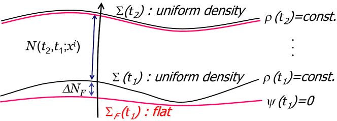
Figure 2: A schematic space-time diagram for the $\Delta N$ formula. The slicing that interpolates between $\Sigma(t_{1})$ and $\Sigma(t_{2})$ is the uniform density slicing, while the relevant slicing for the $\Delta N$ formula is the one that starts from the flat slice $\Sigma_{F}(t_{1})$ and ends on the uniform density slice $\Sigma(t_{2})$. The curvature perturbation on the final hypersurface $\Sigma(t_{2})$ is given by the difference in the $e$-folding number from $\Sigma_{F}(t_{1})$ to $\Sigma(t_{2})$ and that from $\Sigma(t_{1})$ to $\Sigma(t_{2})$.

This is a non-linear version of the $\Delta N$ formula that generalises the first-order result of Sasaki and Stewart

Now we specialise to the case $P=P(\rho)$. In this case, Eq. (22) reduces to

$$\psi(t_{2},x^{i})-\psi(t_{1},x^{i})=-\ln\left[\frac{a(t_{2})}{a(t_{1})}\right]-\frac{1}{3}\int^{\rho(t_{2},x^{i})}_{\rho(t_{1},x^{i})}\frac{d\rho}{\rho+P}\,.$$ (25)

Thus, there is a conserved quantity, which is independent of the choice of time-slicing, given by

$$-\zeta(x^{i})\equiv\psi(t,x^{i})+\frac{1}{3}\int_{\rho(t)}^{\rho(t,x^{i})}\frac{d\rho}{\rho+P}\,.$$ (26)

In the limit of linear theory, this reduces to the conserved curvature perturbation in the uniform-density, uniform-Hubble, or the comoving slicing,

$$-\zeta(x^{i})={\cal R}_{c}(x^{i})=\psi(t,x^{i})+\frac{\delta\rho(t,x^{i})}{3(\rho+P)}\,,$$ (27)

where ${\cal R}_{c}$ is the curvature perturbation on the comoving slices SaSt95 .

4 conclusion

We have investigated the behavior of nonlinear cosmological perturbations on superhorizon scales by invoking the gradient expansion. Already at lowest order in the expansion, we have obtained some non-trivial, very useful results. They are summarized as follows:

• The Friedmann equation for a spatially flat universe holds locally (on scales of the Hubble horizon size), no matter how big the perturbation is on superhorizon scales. A direct consequence of this is that there will be no backreaction effect from super-Hubble perturbations on local (horizon-size) physics. Local physics is determined solely by local physics.

• There exists a non-linear generalization of $\zeta$, which describes the curvature perturbation on uniform density slices, which is conserved for a barotropic fluid on super-Hubble scales.

• There exists a non-linear generalization of $\Delta N$ formula, which relates the final amplitude of the curvature perturbation to the difference in the $e$-folding number between ’flat’ and uniform density slices at an initial epoch (which may be chosen arbitrarily provided that the comoving scale of interest is beyond the Hubble-horizon scale). This formula may be useful in evaluating non-Gaussianity from inflation.

In this report, we only discussed the properties of nonlinear perturbations on superhorizon scales at lowest order in the gradient expansion. However, in non-standard models of inflation, such as in a non-slow-roll model, the second order corrections in the gradient expansion is known to be important already in linear perturbation theory Starobinsky:1992ts ; Leach:2001zf . Thus extending the present analysis to second order in the gradient expansion will be necessary to deal with more general cases. This issue is under investigation YTanaka .

References

- (1) C. L. Bennett et al., arXiv:astro-ph/0302207.
- (2) G. Hinshaw et al., arXiv:astro-ph/0302217.
- (3) D. N. Spergel et al. [WMAP Collaboration], arXiv:astro-ph/0302209.
- (4) E. Komatsu et al., arXiv:astro-ph/0302223.
- (5) J. M. Bardeen, Phys. Rev. D 22, 1882 (1980).
- (6) H. Kodama and M. Sasaki, Prog. Theor. Phys. Suppl. 78, 1 (1984).
- (7) V. F. Mukhanov, L. R. W. Abramo and R. H. Brandenberger, Phys. Rev. Lett. 78, 1624 (1997) [arXiv:gr-qc/9609026].
-
(8)
J. A. Tauber, Adv. Space Res. 34 (2004) 491.
http://www.rssd.esa.int/index.php?project=PLANCK - (9) E. Barausse, S. Matarrese and A. Riotto, Phys. Rev. D 71, 063537 (2005) [arXiv:astro-ph/0501152].
- (10) E. W. Kolb et al., arXiv:hep-th/0503117.
-
(11)
V. A. Belinsky, I. M. Khalatnikov and E. M. Lifshitz,
Adv. Phys. 19, 525 (1970).
K. Tomita, Prog. Theor. Phys. 48, 1503 (1972).
D. S. Salopek and J. R. Bond, Phys. Rev. D 42 (1990) 3936.
K. Tomita and N. Deruelle, Phys. Rev. D 50, 7216 (1994).
N. Deruelle and D. Langlois, Phys. Rev. D 52, 2007 (1995) [arXiv:gr-qc/9411040].
M. Shibata and M. Sasaki, Phys. Rev. D 60, 084002 (1999) [arXiv:gr-qc/9905064].
I. M. Khalatnikov et al., JCAP 0303, 001 (2003) [arXiv:gr-qc/0301119].
G. I. Rigopoulos and E. P. S. Shellard, Phys. Rev. D 68, 123518 (2003) [arXiv:astro-ph/0306620].
G. I. Rigopoulos and E. P. S. Shellard, [arXiv:astro-ph/0405185].
D. Langlois and F. Vernizzi, arXiv:astro-ph/0503416. - (12) D. H. Lyth, K. A. Malik and M. Sasaki, JCAP 0505, 004 (2005) [arXiv:astro-ph/0411220].
- (13) D. H. Lyth and D. Wands, Phys. Rev. D 68, 103515 (2003) [arXiv:astro-ph/0306498].
-
(14)
H. Noh and J. c. Hwang,
Class. Quant. Grav. 22, 3181 (2005)
[arXiv:gr-qc/0412127].
J. c. Hwang and H. Noh, Phys. Rev. D 72, 044011 (2005) [arXiv:gr-qc/0412128]. - (15) C. M. Hirata and U. Seljak, arXiv:astro-ph/0503582.
- (16) D. Wands, K. A. Malik, D. H. Lyth and A. R. Liddle, Phys. Rev. D 62, 043527 (2000) [arXiv:astro-ph/0003278].
- (17) M. Sasaki and E. D. Stewart, Prog. Theor. Phys. 95, 71 (1996) [arXiv:astro-ph/9507001].
- (18) A. A. Starobinsky, JETP Lett. 55, 489 (1992) [Pisma Zh. Eksp. Teor. Fiz. 55, 477 (1992)].
- (19) S. M. Leach, M. Sasaki, D. Wands and A. R. Liddle, Phys. Rev. D 64, 023512 (2001) [arXiv:astro-ph/0101406].
- (20) Y. Tanaka and M. Sasaki, work in progress.