Predictions and Strategies for Integral-Field Spectroscopy of High-Redshift Galaxies

Abstract

We investigate the ability of infrared integral-field spectrographs to map the velocity fields of high redshift galaxies, presenting a formalism which may be applied to any telescope and imaging spectrograph system. We discuss the 5$\sigma$ limiting line fluxes which current integral-field spectrographs will reach, and extend this discussion to consider future large aperture telescopes with cryogenically cooled adaptive reimaging optics. In particular, we simulate observations of spectral line emission from star-forming regions at redshifts $z=0.5$ to 2.5 using a variety of spatial sampling scales and give predictions for the signal-to-noise ratio expected as a function of redshift. Using values characteristic of the W.M. Keck II telescope and the new OH-Suppressing InfraRed Imaging Spectrograph (OSIRIS) we calculate integral-field signal-to-noise ratio maps for a sample of $U_{n}G{\cal R}$ color-selected star-forming galaxies at redshift $z\sim 2-2.6$ and demonstrate that OSIRIS will be able to reconstruct the two-dimensional projected velocity fields of these galaxies on scales of 100 mas ($\sim$ 1 kpc at redshift $z\sim 2$). With signal-to-noise ratios per spatial sample up to $\sim$ 20, OSIRIS will in some cases be able to distinguish between merger activity and ordered disk rotation. Structures on scales smaller than 1 kpc may be detected by OSIRIS for particularly bright sources, and will be easy targets for future 30m class telescopes.

1. INTRODUCTION

As the available instrumentation on large telescopes has pushed observations into the near-infrared (NIR), the denizens of the so-called “redshift desert” from $z\sim 1.4-2.5$ have increasingly become targets of concerted study. Observations suggest that the morphological chaos of the $z\sim 3$ universe evolves into the familiar modern-day Hubble sequence by redshift $z\sim 1$ (e.g. Giavalisco et al. 1996, Papovich et al. 2005), and the redshift $z\sim 2$ population is likely to contain a wide assortment of galactic types as protogalactic merging activitity transitions to kinematically ordered evolution. It often proves difficult however to distinguish starbursting galaxies with an ordered disk morphology from those actively experiencing protogalactic assembly since the relevant angular scales are barely resolved under typical ground-based seeing conditions, and the rest-frame UV light (e.g. as observed in the optical by the Hubble Space Telescope) is dominated by emission from bright, clumpy star-forming regions.

Long-slit nebular emission line spectroscopy has enabled velocity curves to be derived for a sample of high-redshift galaxies (e.g. Pettini et al. 2001, Lemoine-Busserolle et al. 2003, Moorwood et al. 2003, Erb et al. 2003, Erb et al. 2004), giving some insight into the kinematic properties of these sources and suggesting that massive disk systems may be present out to at least redshift 2.5. However, ground-based long-slit spectroscopy suffers from severe atmospheric seeing problems (as demonstrated by Erb et al. 2004), and recovered velocity curves for morphologically selected potentially disk-like galaxies at redshift $z\sim 2$ often show little to no spatially resolved velocity shear (Erb et al. 2004). One possible explanation for this lack of velocity shear may be that these sources are composed of proto-galactic fragments of angular size below the typical seeing limit ($\sim 0\farcs 5$ in the $K$-band).

Given the small apparent angular size of these sources (radius $r\lesssim 1\farcs 0$) compared to that of the seeing disk ($\Theta_{\rm seeing}\approx 0\farcs 5$), high spatial resolution data from ground-based telescopes has only recently become available through the aid of adaptive-optics (AO) technology. The advent of integral-field spectrographs (IFS) on 10m-class telescopes equipped with laser-guide star adaptive optics systems offers the new possibility of mapping the kinematics of galaxies at $z\sim$ 2 on the scale of tenths of an arcsecond or less. Not only can such AO-fed spectrographs mitigate the seeing-induced uncertainties inherent in velocity curves derived from long-slit spectra, but their integral-field capability will provide two-dimensional velocity maps from which it may be possible to reconstruct the kinematic profiles of these galaxies on scales of a few hundred parsecs.

Recent years have seen a rapid increase in the number of optical/NIR integral-field spectrographs capable of studying the velocity fields of high redshift galaxies (Table 1), and these instruments are starting to yield kinematic maps of large galaxies from redshifts $z=$ 0.1 (Swinbank et al. 2005a) and 0.5 (Flores et al. 2004) up to $z=$ 2.4 (Swinbank et al. 2005b). In this contribution, we outline an observing strategy for integral-field IR spectroscopy of high redshift galaxies, treating the case of a general telescope + IFS system in §2. In §3 we narrow our discussion to concentrate on simulating the capabilities of the OSIRIS spectrograph on the W.M. Keck II telescope, and predict the signal-to-noise (S/N) ratios expected for observations of nebular line emission from star-forming regions with redshifts from $z\sim 0.5-2.5$. We explore the relative merits of available lenslet scales and observable spectral emission lines, and assess the ability of OSIRIS to obtain spatially resolved velocity information from $U_{n}G{\cal R}$ color-selected galaxies at redshift $z\sim 2$ - 2.5 in the Hubble Deep Field North (i.e. the “BX” sample defined by Steidel et al. 2004 and Adelberger et al. 2004). Finally, in §4 we use characteristics typical of the OSIRIS spectrograph to investigate the limiting line fluxes detectable from an arbitrary source using current generation spectrographs, extending this discussion to consider next-generation telescopes and cryogenically cooled optical systems.

Table 1Current Optical/IR Integral-Field Spectrographs

Spectrograph	Telescope	Optical	NIR	AO	Reference
GIRAFFE	VLT	yes	no	no	Hammer et al. (1999)
GMOS	Gemini	yes	no	NGS	Davies et al. (1997)
GNIRS	Gemini	no	yes	no	Allington-Smith et al. (2004)
INTEGRAL	WHT	yes	no	NGS	García-Lorenzo et al. (2000)
NIFS	Gemini	no	yes	NGS	McGregor et al. (2003)
OSIRIS	Keck II	no	yes	LGS	Larkin et al. (2003)
SAURON	WHT	yes	no	no	Bacon et al. (2001)
SINFONI/SPIFFI	VLT	no	yes	LGS	Tecza et al. (1998)
UIST	UKIRT	no	yes	no	Ramsay Howat et al. (1998)

We assume a cosmology in which $h=0.7$, $\Omega_{m}=0.3$, $\Omega_{\Lambda}=0.7$.

2. METHOD

Integral-field (or multi-object) spectrographs may have optical designs ranging from a simple objective prism to a more complex fiber-fed, lenslet-based, or image-slicing configuration. We tailor our discussion specifically to the case of an imaging lenslet array, in which each of a closely spaced array of lenslets disperses a spectrum in a staggered pattern onto a detector (a good introduction to this technique is given by Bacon et al. 1995). Our formalism is presented with such a lenslet-type spectrograph in mind, but may be easily modified for both image-slicing and fiber-type spectrographs.

2.1. Signal Estimation

2.1.1 Estimating Background Count Rates

We adopt the Gemini Observatory model for the Mauna Kea near-IR sky brightness spectrum (spectral resolution ${\cal R}\sim 2000$) which incorporates zodiacal emission (from a 5800 K blackbody), atmospheric emission (from a 250 K blackbody), and radiation from atmospheric OH molecules. In addition to these components we introduce models of the thermal blackbody emission from warm reflective surfaces in the light path. The telescope mirrors and the adaptive reimaging optics are modelled as 270 K blackbodies with net emissivities $\epsilon=1-\eta$ (where $\eta$ is the transmission coefficient of the component).

Using the Planck blackbody function, the photon flux due to thermal emission from these components is

$$f_{\lambda}=\epsilon\,\alpha^{2}\,\frac{2\,c}{\lambda^{4}}\frac{1}{e^{hc/\lambda kT}\,-\,1}\,{\rm photons}\,{\rm s}^{-1}\,{\rm cm}^{-2}\,{\rm cm}^{-1}\,{\rm arcsec}^{-2}$$ (1)

where $f_{\lambda}$ is the spectral flux at wavelength $\lambda$, $\alpha=4.85\times 10^{-6}$ is a scale factor representing the number of steradians per square arcsecond, $T$ is the temperature of the component in degrees Kelvin, and the remaining symbols $c,h$ and $k$ are standard physical constants.

The corresponding total electron count rate per detector pixel per lenslet ($R_{\rm BG}$, electrons s^-1 lenslet^-1 pixel^-1) from these three background sources (Gemini sky brightness model, telescope emissivity, and AO system emissivity) is given by

$$R_{\rm BG}(\lambda)=(f_{\lambda,{\rm sky}}\,\eta_{\rm tel}\,\eta_{\rm AO}+f_{\lambda,{\rm tel}}\eta_{\rm AO}+f_{\lambda,{\rm AO}})\,\eta_{\rm spec}(\lambda)A\,a^{2}\frac{P}{{\cal N}_{1}}$$ (2)

where $f_{\lambda,{\rm sky/tel/AO}}$ represents the photon flux from the sky/telescope/AO system respectively in photons s^-1 cm^-2 cm^-1 as^-2, $\eta_{\rm tel}$ is the throughput of the telescope optics, $\eta_{\rm AO}$ is the throughput of the AO system, $\eta_{\rm spec}(\lambda)$ is the throughput of the spectrograph (a complicated function of $\lambda$ including the throughput of the spectrograph blaze function, filter transmission, detector response, and optical throughput additional components), $A$ is the telescope collecting area, $a$ is the angular lenslet size (in arcseconds), $P$ is the pixel scale (wavelength coverage per pixel), and ${\cal N}_{1}$ is the spatial width of each spectrum in detector pixels.

2.1.2 Estimating Source Count Rates

The source count rate in a given emission line may be estimated by scaling a finely sampled (i.e. with spatial resolution at least as fine as the desired lenslet scale) map of the source morphology by the total emission line flux of the source. While H$\alpha$ maps of high redshift galaxies are generally unavailable, H$\alpha$ emission often correlates well with the FUV (1500Å) morphology, as demonstrated for late-type local galaxies by Gordon et al. (2004), Kennicutt et al. (2004), and Lee et al. (2004), and it is often a reasonable approximation to use a FUV flux map to represent the H$\alpha$ flux distribution (although cf. Conselice et al. 2000). The FUV flux can readily be observed by the Hubble Space Telescope’s Advanced Camera for Surveys (HST-ACS) since rest-frame FUV emission is redshifted into the $B$-band for sources at redshift $z\sim 2-2.6$, and we therefore use images of our target galaxies in the GOODS-N field which are publically available from the HST-ACS data archives. These images are ideal for studying the morphology of the target galaxies on angular scales of less than an arcsecond since the point-spread function of the ACS data is about 125 mas (Giavalisco et al. 2004).

These FUV flux maps are resampled into pixel maps with a pixel size corresponding to the desired lenslet scale, and the sum of the pixel values is rescaled by the total line flux of the source divided by the average photon energy to obtain a grid of line fluxes $f_{\lambda,{\rm source}}$ (photons s^-1 cm^-2 lenslet^-1) for each lenslet. Since the adopted ACS flux maps have already been sky-subtracted we assume that all pixels within a given region with fluxes above zero-threshold represent source emission, and find the total FUV source flux by simply summing all such pixels. The average electron count rate per detector pixel (electrons s^-1 lenslet^-1 pixel^-1) is then calculated in analogy to Equation 2 as

$$R=f_{\lambda,{\rm source}}\,\eta_{\rm atm}(\lambda)\,\eta_{\rm tel}\,\eta_{\rm AO}\,\eta_{\rm spec}(\lambda)\,\frac{A}{\Delta\lambda}\,\frac{P}{{\cal N}_{1}}$$ (3)

where $\Delta\lambda$ is the full width at half maximum (FWHM) of the spectral line (computed as the quadrature sum of the line width due to source velocity dispersion $\sigma_{\rm v}$ and from the finite spectrograph resolution) and $\eta_{\rm atm}(\lambda)$ is the atmospheric transmission as a function of wavelength, for which we adopt the Mauna Kea transmission spectra generated by Lord 1992.

2.1.3 Adaptive-Optics and Seeing Corrections to Count Rates

We now take into account the effects of realistic AO performance and losses to the atmospheric seeing halo (the net throughput of the AO system was already taken into account in §2.1.1 and 2.1.2). The flux in each lenslet is resampled uniformly into a grid of $x$ $\times$ $x$ squares, and the approximation made that the flux in each grid square (before incidence upon the Earth’s atmosphere) may be described as a point source. After traversing both the atmosphere and the AO system, the light from this point source is divided between a diffraction-limited core and a seeing-limited halo, the fluxes of which are given by

$$f_{\rm diffraction}= {\cal S}\times f_{\rm total}$$ (4)

$$f_{\rm seeing}= (1-{\cal S})\times f_{\rm total}$$ (5)

where ${\cal S}$ is the strehl of the AO correction. Assuming that the net wavefront error of the adaptive optics system $\sigma_{\rm wfe}$ is constant, strehl as a function of wavelength is given by

$${\cal S}=e^{-(2\pi\sigma_{\rm wfe}/\lambda)^{2}}$$ (6)

Both the seeing-limited halo and diffraction-limited core may be approximately represented by two-dimensional Gaussian profiles with $\sigma_{\rm halo}=\frac{\theta_{\rm seeing}}{2.4}$ and $\sigma_{\rm core}=\frac{1.22\,\lambda/D}{2.95}$ (where $D$ is the diameter of the telescope’s primary mirror). The core and halo light profiles from each grid square may be integrated over each lenslet to generate an observed flux distribution which incorporates both losses to the seeing halo from a given lenslet and gains from the seeing halos of neighboring lenslets.

Since this procedure assumes that light lost to the seeing halo of one lenslet is recovered by surrounding lenslets, it is possible that all losses to the seeing halo from a given lenslet may be regained from spill-over flux from the halos of neighboring lenslets if the intrinsic flux in these neighbors is suitably high. However, this flux will generally be a source of additional background noise - if the flux is spilled from a region of the source with a very different line-of-sight velocity it will contribute this flux at the corresponding wavelength and hinder precise measurement of the spectral peak of flux originating from a given lenslet. Modeling this complex effect in detail requires a priori knowledge of the velocity substructure of the source, and we therefore generally assume that all such spilled flux adds to the noise of the observation rather than the signal. In §2.2 and §3.4 where we adopt specific velocity models however, spilled light is treated comprehensively as a function of both angular position and wavelength.

2.1.4 Estimating Signal-to-Noise Ratios

Using the quantities derived it is possible to calculate the S/N ratio expected for detection of a particular spectral line in each lenslet. We use the standard equation

$$\frac{S}{N}=\frac{R\,{\cal N}_{1}\,{\cal N}_{\rm spec}\,t}{\sqrt{(R+R_{\rm BG}+R_{\rm DK})\,{\cal N}_{1}\,{\cal N}_{\rm spec}\,t+N_{\rm RD}^{2}\,(t/t_{0})\,{\cal N}_{1}\,{\cal N}_{\rm spec}}}$$ (7)

where ${\cal N}_{\rm spec}$ is the number of spectral pixels summed (i.e. the FWHM of the spectral line in pixels), $R_{\rm DK}$ is the dark current count rate in e^- s^-1 pixel^-1, $N_{\rm RD}$ is the detector read noise in e^- pixel^-1, $t$ and $t_{0}$ are the total and individual exposure times respectively, and all other quantities have been previously defined.

2.2. Spectral Synthesis

Simply detecting an emission line with some confidence does not guarantee that its centroid can be measured with great accuracy, and we therefore generate artificial spectra and attempt to measure their centroids using techniques which will be applied to observational data to effectively simulate the recovery of velocity substructure.

Defining a spectral vector with one element for each spectral pixel (i.e. summing over the ${\cal N}_{1}$ detector pixels to create a 1-dimensional spectrum), it is easy to generate a simulated spectrum from the counts as a function of wavelength by introducing noise according to Poisson statistics. Using this simulated spectrum (or an observed spectrum which has been precisely wavelength calibrated using the bright OH spectral features), the background signal $N_{BG}=(R+R_{\rm BG}+R_{\rm DK})\,{\cal N}_{1}\,{\cal N}_{\rm spec}\,t+N_{\rm RD}^{2}\,(t/t_{0})\,{\cal N}_{1}\,{\cal N}_{\rm spec}$ due to read noise, dark current, and the sky background may be subtracted off to determine the sky-subtracted counts as a function of wavelength for the source. This spectrum may be further processed to obtain velocity centroids using standard routines. Hand-processing by an experienced individual appears to be the most reliable method of measuring velocity centroids, although such a method is impractically time-consuming for extensive simulations with hundreds of spectra apiece. Instead, we adopt an automated routine which fits a gaussian profile to the background-subtracted spectra using a Levenberg-Marquardt fitting algorithm (a non-linear least-squares regression algorithm similar to that used in the standard IRAF routine splot) and measures the velocity shift of the peak flux from the systemic redshift. This method is found to perform reliably for most spectral features with S/N ratios $>3$, although some particularly faint features which are not handled well by this automated method may still yield useful information when individually hand-processed.

We note that for the case of spectrographs whose output is in the form of data cubes, one-dimensional observational spectra may be extracted for each spatial element, and may then be processed in entirely the same manner as these simulated spectra.

3. SIMULATED OBSERVATIONS WITH OSIRIS

The simulation method described in the previous section has been outlined in a general manner so that it may be applied to any telescope and integral-field spectrograph system. We now proceed to adopt characteristics typical of the W.M. Keck II telescope and OSIRIS spectrograph in order to quantify the performance capability expected from this system for the study of high-redshift galaxies. In §3.1 we describe the site, telescope, and spectrograph characteristics, and in §3.2 we explore the expected detection limits of OSIRIS for observations of nebular line emission from typical star-forming regions at redshifts $z=0.5-2.5$. In §3.3 we present integral-field S/N ratio maps for selected $z\sim 2-2.6$ star-forming galaxies in the GOODS-N field and explore the integration times and lenslet scales required to achieve significant detections. Finally, in §3.4 we explore the ability of OSIRIS to recover the velocity substructure of these sources assuming disparate kinematic models. We note that the assumed characteristics of the OSIRIS spectrograph are preliminary results based upon commissioning data, and the results of our analysis should therefore be scaled accordingly to reflect the final well-determined specifics of the instrument once such information is available.

3.1. The OSIRIS Spectrograph

3.1.1 Mechanical Overview

OSIRIS (OH-Suppressing InfraRed Imaging Spectrograph) is an integral-field spectrograph designed and built at UCLA for the Keck II telescope (Larkin et al. 2003), and is presently in the initial stages of commissioning during the 2005 observing season. The spectrograph employs reimaging optics to select between lenslet scales of 20, 35, 50, and 100 mas and uses a low dark-current Hawaii-2 HgCdTe 2048 $\times$ 2048 IR detector array. OSIRIS is designed to work in conjunction with the Keck-II laser guide star (LGS) AO system since the vast majority of targets (about $\sim 99$% of the sky) are too distant from a suitably bright star to permit natural guide star (NGS) observations. Characteristic parameters for the Keck II telescope, LGS AO system, and OSIRIS spectrograph are summarized in Table 2. The spectrograph parameters given are based upon values provided in the OSIRIS pre-ship report (J. Larkin, private communication).

Table 2Keck/OSIRIS System Characteristics

Parameter	Symbol	Value
Telescope/AO characteristics
AO throughput	$\eta_{\rm AO}$	65%
Collecting area	$A$	$7.85\times 10^{5}$ cm2
$K$-band diffraction limit	$\theta_{\rm diff}$	55 mas
$K$-band seeing	$\theta_{\rm seeing}$	550 mas
Telescope throughput	$\eta_{\rm tel}$	80%
Wavefront error	$\sigma_{\rm wfe}$	337 nm
OSIRIS Characteristics
Average OSIRIS throughput	$\eta_{\rm spec}$	15% ($z$-$H$ bands)
		20% ($K$ band)
Average system throughput	$\eta$	8% ($z$-$H$ bands)
		10% ($K$ band)
Dark current	$R_{\rm DK}$	.03 e- s-1 pixel-1
Grating blaze	$\cdots$	6.5 $\micron$
Read noise	$N_{\rm RD}$	3 e- pixel-1
Spectral length	${\cal N}_{2}$	1600 pixels (broadband)
		400 pixels (narrowband)
Spectral resolution	${\cal R}$	3900 (20, 35, 50 mas lenslets)
		3400 (100 mas lenslets)
Spectral width	${\cal N}_{1}$	3 pixels

OSIRIS uses broad- and narrow-band order-sorting filters to select the wavelength range imaged on the detector; the available four broadband IR filters (outlined in Table 3) are chosen to correspond to the regions of high throughput in orders $n=3-6$ of the spectrograph grating (blazed at 6.5 µm). Operating in broad-band mode, OSIRIS is capable of producing spectra from 16 x 64 lenslets for a total of 1024 spectra with 1600 spectral pixels each. OSIRIS is also capable of operating in narrow-band mode using 19 narrow-band filters which together span the same range of wavelengths as the broadband filter set. This narrow-band mode will generally be more useful for targeted velocity studies of high-redshift galaxies, for which velocity-shifted nebular emission lines are expected to fall within a few angstroms of the systemic value. In this mode, spectra from 48 x 64 lenslets can fit on the detector for a total of 3072 spectra comprised of 400 spectral pixels each. The resulting fields of view for broadband and narrow-band operation at each of the four available lenslet scales are given in Table 4.

Table 3OSIRIS Broadband Filters and Effective Model Sky Surface Brightness

Band	Wavelength ($\micron$)	$\eta_{\rm filter}$	$\mu_{\rm AB}$	$\mu_{\rm Vega}$	$f_{\lambda}$
$z$	.98 — 1.20	0.73	17.9	17.3	3.64044
$J$	1.18 — 1.44	0.81	17.8	16.8	3.33187
$H$	1.47 — 1.80	0.79	18.0	16.6	2.09761
$K$	1.96 — 2.40	0.81	15.2	13.3	20.5934

In the interests of integration time, a suitably large field of view must be chosen so that a reasonable number of lenslets are imaging both the science target and the off-source background sky (for calibration purposes) simultaneously. In narrow-band mode, this means that at least 5% of the lenslets must have negligible flux from the science target in order to calculate a background signal with an uncertainty of less than 10% of the Poisson shot noise. Most redshift $z\sim 2$ star-forming galaxies have radial size $\sim$ 1 arcsecond or less, resulting in a source area of

$$A_{\rm source}\lesssim\pi\left(\frac{1\,{\rm arcsecond}}{a}\right)^{2}\,\,\,{\rm lenslets}$$ (8)

where $a$ is again the lenslet scale in arcseconds. Operating at all except the finest sampling scales of $a=20$ mas, these sources cover considerably less than the total number of lenslets available over the field of view, indicating that accurate estimation of the background flux will be possible with no additional pointings. Studies using lenslet scales of $a=20$ mas will require greater caution in the placement of their fields of view to ensure reasonable background coverage, although as will be demonstrated in §3.3 these small sampling scales are unlikely to be of great utility for OSIRIS observations of $z\sim 2$ galaxies anyway.

Table 4Available OSIRIS Angular Lenslet Scales and Fields of View.

Lenslet Scale	Broadband FOV	Narrowband FOV
0.02	0.32 $\times$ 1.28	0.96 $\times$ 1.28
0.035	0.56 $\times$ 2.24	1.68 $\times$ 2.24
0.05	0.8 $\times$ 3.2	2.4 $\times$ 3.2
0.10	1.6 $\times$ 6.4	4.8 $\times$ 6.4

3.1.2 Mauna Kea/OSIRIS Noise Characteristics

The model background sky brightness as a function of wavelength is calculated as outlined in §2.1.1 for typical Keck II and AO system characteristics and is plotted in Figure 1. Note that for sake of clarity we suppress individual OH emission lines which are visibly separated from neighboring lines by a region of inter-line background, since it will in general be possible to work around these emission features. Effective sky surface brightnesses corresponding to this background spectrum are given in Table 3.

Figure 1.— Model effective background sky spectrum for Keck II incorporating the Gemini model for zodiacal light and atmospheric emission (${\cal R}\,\sim$ 2000), a 35% emissivity in the AO system, and a 20% emissivity in the telescope optics (90% throughput for both the primary and secondary mirrors) at temperature $T=270$ K. Spectrally dense OH emission line regions appear as spikes since a spectrograph with resolution ${\cal R}=2000$ will not be able to reach inter-line background levels in these regions of severe contamination. The dip around 1.4 $\micron$ is due to high atmospheric opacity. Redshifts for which H$\alpha$ emission falls at a particular wavelength are indicated along the top axis of the plot.

It is informative to compute the relative contribution of detector read noise, dark current, and background radiation in determining the total noise in an exposure. As given in Table 2, the read noise for the Hawaii-2 infrared detector array is $N_{\rm RD}\sim$ 3 electrons pixel^-1 (after multiple correlated double samples), with a dark current of $R_{\rm DK}=$ 0.03 electrons s^-1 pixel^-1. Using the model background spectrum (Fig. 1), it is possible to calculate the minimum exposure time $t_{\rm min}$ required for read noise to become a negligible contributor to the total noise budget,

$$t_{\rm min}=\frac{N_{\rm RD}}{R_{\rm DK}+R_{\rm BG}}$$ (9)

Figure 2.— Minimum integration time required for detector dark current $+$ background counts to equal the detector read noise for lenslet scales of 100 (black line), 50 (red line), 35 (green line), and 20 mas (blue line).

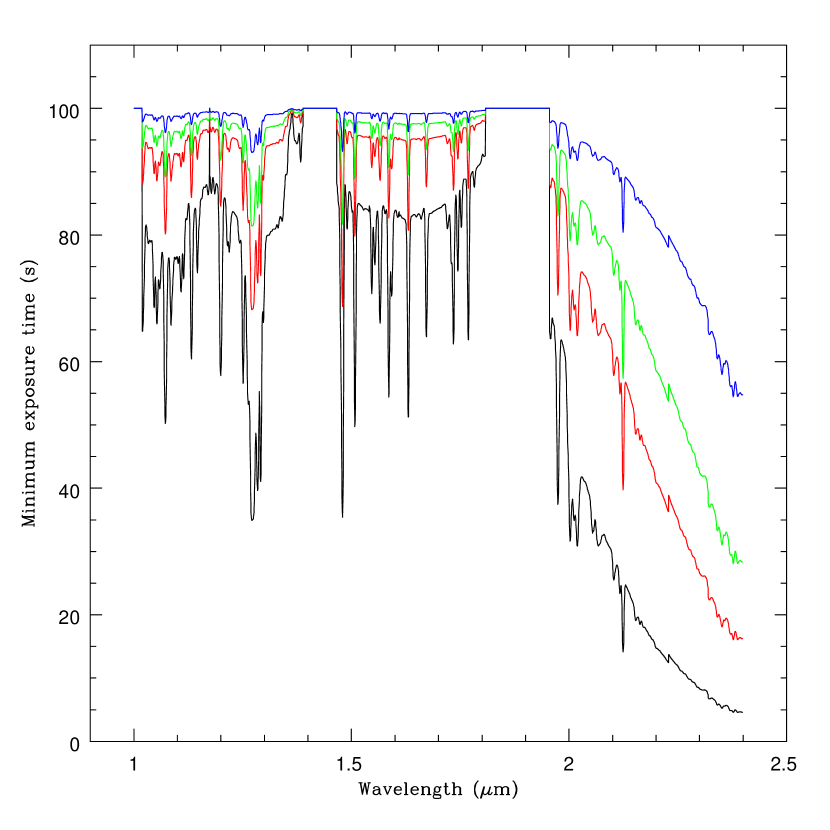
Figure 2 plots the minimum exposure time as a function of wavelength for lenslet scales of 20, 35, 50, and 100 mas. Note that for wavelengths where background radiation is negligible compared to the dark current $t_{\rm min}$ approaches 100 seconds (since $N_{\rm RD}/R_{\rm DK}=$ 100 seconds), while at wavelengths for which $t_{\rm min}<50$ seconds the background radiation dominates over the dark current. In order to minimize the contribution of detector read noise to our simulations we fix invidual exposure times at $t_{0}=$ 900 seconds, although we note that shorter times could be chosen on the basis of Figure 2 if long observations prove problematic due to technical difficulties such as LGS-shuttering from beam collisions with other Mauna Kea observatories (S. Kulkarni, private communication).

Figure 3.— Relative S/N ratios achieved binning data from 50, 35, and 20 mas lenslets (solid curves, top to bottom respectively) to 100 mas, as compared to data taken using 100 mas lenslets. Redshifts for which H$\alpha$ emission falls at a particular wavelength are indicated along the top axis of the plot.

Ideally, observations could be conducted using the finest available lenslet scale for which the field of view covers the entire target, since (even if the signal is too low to usefully measure on such a fine scale) the results may be spatially binned to coarser scales. In practice however detector noise often imposes severe penalties on fine sampling scales, introducing noise into the binned sample. Using our characterization of the Keck/OSIRIS noise budget, we assess the utility of such binning as a function of wavelength by plotting the fractional change in the S/N ratio obtained by binning data from the three smaller lenslet scales to 100 mas (Fig. 3). These calculations adopt an individual exposure time of 900 seconds, and assume that the flux from the desired target is negligible compared to the background flux. We note that for wavelengths longward of 2.3 $\micron$ the S/N ratios achieved for binning 50 mas lenslets to 100 mas scales is about 90% of that achived using actual 100 mas sampling, suggesting that for long wavelength observations it may be worthwhile to use small lenslets even for faint sources (although finer sampling will come at the cost of decreased field-of-view).

3.2. Observing Star-Forming Regions at Intermediate to High Redshifts

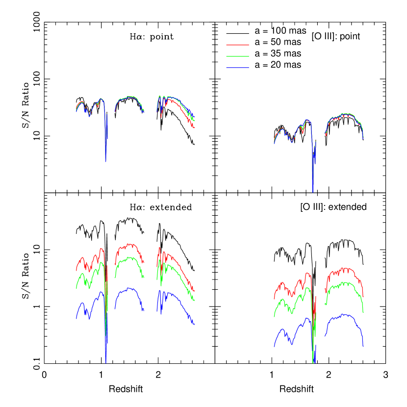
To assess the anticipated performance of OSIRIS we estimate the S/N ratios expected for observations of star-forming regions at redshifts $z=$ 0.5 - 2.5, considering the cases of a spatially unresolved (i.e. pointlike), isolated star-forming region, and a spatially extended source with a physical diameter of 1 kpc. In each case it is assumed that the star-formation rate is 1 $M_{\odot}$ yr^-1 (assuming a Salpeter IMF this corresponds to an H$\alpha$ luminosity of $1.27\times 10^{41}$ erg s^-1 from Kennicutt 1998), and that the velocity dispersion is negligible within a single spatial sample. In each of these cases both simulated H$\alpha$ and [O III] $\lambda 5007$ emission lines (assuming [O III]/H$\alpha$ $\sim$ 1) are artificially observed to calculate the expected S/N ratio expected in the peak lenslet at sampling scales of 100, 50, 35, and 20 mas. These simulations take into account the redshift dependence of flux and angular diameter, and the wavelength dependence of the atmospheric seeing, diffraction limit, sky brightness, and AO correction strehl (assuming a fixed wavefront error $\sigma_{\rm wfe}=337$ nm).

Figure 4.— Expected signal-to-noise ratios for 1 hour observations of point and extended (1 kpc diameter) sources with a star formation rate of 1 $M_{\odot}$ yr^-1 using different OSIRIS lenslet scales ($a$). The line flux ratio [O III] ($\lambda 5007$)/H$\alpha$ is taken to be unity, and the velocity dispersion in each spatial sample is assumed to be negligible.

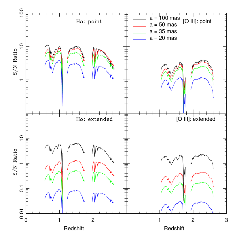
Figure 4 plots the results as a function of redshift for each of the available OSIRIS lenslet scales. In general the shape of the curves reflects the adopted atmospheric and spectrograph transmission spectra, with gaps where atmospheric transmission is particularly poor (OSIRIS filters are designed to cut out these wavelength intervals). The monotonic decrease in the S/N ratio for observations of H$\alpha$ at redshift $z>2.1$ however is due to the rapidly rising thermal contribution to the background radiation in the $K$-band. We note that for point-like sources virtually the same signal level is obtained using both 100 mas and 50 mas sampling scales since nearly the same amount of integrated light is contained within the lenslet, while losses begin to occur on scales of 35 and 20 mas which are below the Keck diffraction limit. In contrast, for extended sources the signal obtained using smaller lenslets is considerably reduced since the lenslets are gathering light from a smaller effective area.

Observations of the rest-frame optical spectra of redshift $z\sim 2$ and $z\sim 3$ Lyman-Break Galaxies (LBGs, e.g. Pettini et al. 2001, Erb et al. 2003) have demonstrated that these galaxies have strong nebular emission lines, particularly [O III] $\lambda$5007 for which the line flux ratio [O III]/H$\alpha$ can be close to unity for relatively metal-poor ($<$ 0.5 solar) sources. Since the thermal background rises rapidly in the $K$ band (Fig. 1), this strong [O III] emission can present an appealing observational alternative to H$\alpha$ since it falls in the $H$ band (which has a lower thermal background) for redshifts $z\approx 1.9-2.6$. However the exponential decrease of strehl with shorter wavelengths, paired with the fact that detector dark current rather than thermal background radiation tends to dominate the error budget at most wavelengths and sampling scales, means that as shown in Figure 4 (right panels) it will still be most efficient to observe H$\alpha$ emission for all except those sources at $z>2.5$, or at redshifts for which H$\alpha$ emission is severely attenuated by the atmosphere.

We conclude for redshift $z\sim 2-2.6$ star-forming galaxies (which have typical uncorrected H$\alpha$ star-formation rates of $\sim$ 16 $M_{\odot}$ yr^-1, Erb et al. 2003) that 100 mas sampling of H$\alpha$ emission with OSIRIS should in general yield fairly comprehensive spatial coverage with an integration time of a few hours (see also §3.3). However, background radiation and detector dark current will largely be prohibitive for obtaining spectroscopic data on scales of 50 mas or below. As described in §3.1.2 though, it may nonetheless be desirable to use such fine sampling scales since: (1) Coarser sampling scales can be reconstructed by binning data, often with relatively little loss of signal strength, and (2) If emission regions visible in the ACS data resolve into point-like sources (e.g. giant H II regions or super-star clusters) on scales below the HST-ACS resolution limit the signal on small scales may be larger than anticipated.

3.3. Signal-to-Noise Ratio Maps

In order to reliably reconstruct the velocity profile of a galaxy it will be necessary to obtain spectra with high S/N ratios over many lenslets. Using the tools developed so far we generate theoretical S/N ratio maps for four of the $z\sim 2-2.6$ starforming galaxies observed by Erb et al. (2004) to illustrate the spatial extent of the data which Keck/OSIRIS will be capable of providing.

Table 5Parameters of Selected Galaxies

Galaxy	$z_{\rm H\alpha}$	$F_{\rm H\alpha}$	$\sigma_{\rm v}$
BX 1311	2.4843	16.0	88
BX 1332	2.2136	8.8	54
BX 1397	2.1332	10.6	123
BX 1479	2.3745	5.0	46

Using the instrument parameters outlined previously in Table 2, we simulate observations of BX galaxies 1311, 1332, 1397, and 1479 drawn from the Steidel et al. (2004) catalog. These four sources were selected because they all have long-slit H$\alpha$ spectra, two of them (BX 1332, 1397) with actual tilted velocity curves, and generally have elongated or multiple-component morphologies. H$\alpha$ fluxes for these galaxies are estimated using lower limits to the fluxes measured by Erb et al. (2004); motivated by narrowband imaging and continuum spectroscopy of similar sources we estimate a factor of $\sim$ 2 correction to the Erb et al. (2004) values to account for slit losses and non-photometric observing conditions (see Table 5 for a summary of these corrected flux values). The average H$\alpha$ flux of the BX galaxy sample is roughly $\sim 6\times 10^{-17}$ erg s^-1 cm^-2 (Erb et al. 2005), and therefore while BX 1332 and 1397 are slightly brighter than average we note that BX 1479 may be taken as roughly representative of the typical flux of the sample. These H$\alpha$ fluxes are used to scale the ACS $B$-band (F450W) images to generate H$\alpha$ flux maps as described in §2.1.2. In each case we assume that the velocity dispersion is negligible within a single spatial sample.

Figure 5.— Estimated S/N ratio maps for $z\sim 2-2.6$ star forming galaxies BX 1311, 1332, 1397, and 1479. Simulated observations use 100 mas lenslets and image H$\alpha$ emission for 4 hours of total integration time. The velocity dispersion in each spatial sample is assumed to be negligible.

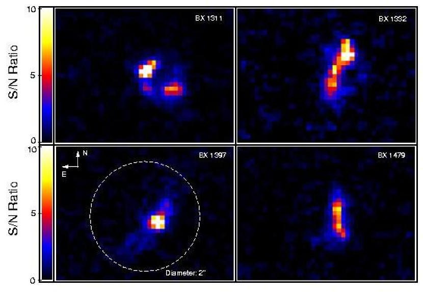
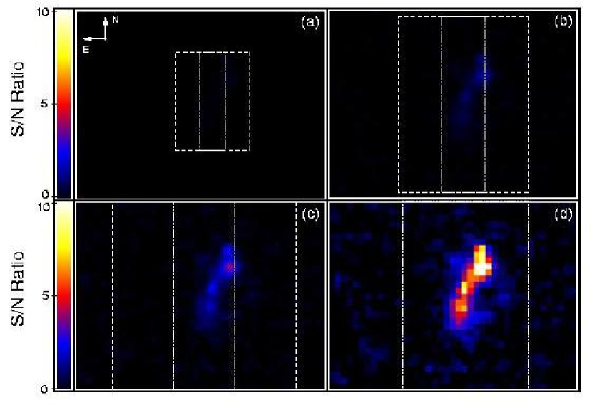
S/N ratio maps of these four galaxies are given in Figure 5, and show that in a four hour integration we expect to obtain numerous spectra with S/N ratios $\gtrsim$ 5 (red pixels) across the source if a lenslet scale of 100 mas is used (as expected on the basis of Fig. 4). In comparison, Figure 6 illustrates the S/N ratios expected in the same integration time for BX 1332 using the four available lenslet scales of 20, 35, 50, and 100 mas (panels a - d respectively). Clearly, 20 and 35 mas sampling scales are unlikely to be of use for observations of $z\sim 2$ galaxies since peak S/N ratios for emission line detection are less than or of order unity in a four hour exposure, indicating that the integration times required to achieve detectable signals are prohibitively large. As demonstrated by panel (c), 50 mas sampling scales could nonetheless prove of use when spatially binned, for brighter sources, or for those sources in which emission regions resolve out into identifiable point sources.

Figure 6.— As Figure 5, but plots show S/N ratio maps for BX 1332 using lenslet scales of 20, 35, 50, and 100 mas (panels a.-d. respectively). OSIRIS broadband and narrowband fields of view (Table 4) for each lenslet scale are overplotted (dotted and dashed lines respectively) for comparison.

In the event that the assumption of negligible velocity dispersion within a single lenslet were to break down (as when observing an AGN), the line emission would be spread over a greater number of detector pixels, increasing the noise in the detection and resulting in S/N ratios somewhat lower than found for unresolved line emission.

3.4. Recovery of Velocity Structure

As described in §2.2, detecting line emission in a given lenslet does not necessarily mean that it will be possible to measure a value of the velocity centroid to within an accuracy necessary for studying velocity substructure (i.e. tens of km s^-1) since severe contamination of the light in a given lenslet by spillover from a bright nearby component may mask the velocity signature. We therefore test how accurately we can expect to reconstruct the velocity field of BX 1332 given two possible kinematic models for the system.

Figure 7.— Observed Keck/NIRSPEC velocity curve of BX 1332 (filled squares, from Erb et al. 2004) overplotted with simulated Keck/NIRSPEC observations assuming rotating disk kinematics (solid line) and a bimodal velocity distribution (dotted line). Model velocities have been uniformly scaled along the vertical axis to precisely match the dynamic range of the observational data.

In a previous study using long-slit Keck/NIRSPEC spectroscopy Erb et al. (2004) observed a tilted velocity curve along the major axis of BX 1332 (Fig. 7, filled squares), but the high degree of correlation among their data points due to atmospheric seeing ($\sim 0.8$ arcsec) meant it was uncertain whether the tilted velocity curve was due to ordered disk rotation, or simply to two clumps merging or otherwise passing each other at some relative velocity. We therefore construct two kinematic models for this source: 1) A disk exhibiting solid-body rotation for which the size, inclination, and position angle are chosen so that the projected ellipsoid roughly traces the contours where the S/N ratio is equal to 3 in Figure 6 (panel d.), 2) A bimodal velocity distribution in which the velocities of the northwest and southeast regions are separated by the total observed velocity gradient ($\sim$ 100 km s^-1). In each case, the intrinsic velocity dispersion within a given spatial sample is assumed to be negligible. These velocity maps are superimposed on the line flux map (generated as described in §3.3) on a pixel-to-pixel basis. While there are many uncertainties and degeneracies in this method the exact set of parameters used for the two models is of little consequence since we are primarily interested in how well we can distinguish between two fundamentally distinct kinematic models on the basis of velocity maps reconstructed from simulated observational data (§2.1.4 and 2.2). This is illustrated in Figure 8, which plots the HST-ACS $B$-band image of BX 1332 (panel a.), the S/N ratio map for spectral line detection (panel b.), and the velocity map recovered from a 4-hour exposure using the techniques described in §2.2 for both rotating disk and bimodal velocity models (panels c. & d. respectively).

Based on long-slit Keck/NIRSPEC observations, it would not be possible to distinguish these two kinematic models. Adopting a rough model of the NIRSPEC spectrograph with spectral resolution ${\cal R}=1400$ in the $K$ band, Figure 7 overplots the Erb et al. (2004) observational data with model velocity curves recovered from simulations assuming a rotating disk model (solid line) and a bimodal velocity model (dotted line). Although these two model velocity curves are generally quite similar, a chi-squared analysis prefers the disk model over the bimodal model with a chi-square probability function of 0.02 compared to $10^{-10}$. However, this distinction is deceptive, since a bimodal velocity model with identical shape but 80% the dynamic range in velocity produces a chi-square fit as good as for the disk model. Since the velocity amplitude of the source is uncertain to within about 20%, we conclude that both rotating disk and bimodal velocity models are equally consistent with the NIRSPEC velocity curve.

Figure 8.— (a) HST-ACS $B$-band image of BX 1332 from the GOODS-N survey. Panel (b) reproduces the S/N ratio map for spectroscopic detection of the galaxy, and panels (c) & (d) respectively show the velocity profiles reconstructed from simulated observational data for rotating disk and bimodal velocity structures. Panels (c) & (d) plot only data from those lenslets with greater than 3$\sigma$ detections of emission line flux, and for which the recovered velocity is within 1000 km s^-1 of the systemic redshift.

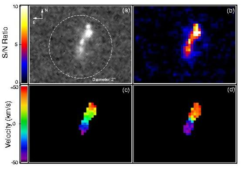
In contrast, with IFS, adaptive optics, and increased spectral resolution, simulations of OSIRIS were able to clearly distinguish between the two models: in panel (c) of Figure 8 the velocity map shows a smooth transition from redshift to blueshift (relative to systemic) over the entirety of the source, while in panel (d) only a few pixels on the boundary between the two clumps give intermediate recovered velocities (since residual atmospheric seeing blurs the light from the two clumps into a slightly broader emission feature at close to the systemic redshift). We therefore conclude that OSIRIS will in some cases be capable of distinguishing between rotating disks and two-component mergers previously indistinguishable with long-slit spectrographs alone. However, BX 1332 is a particularly extended source, which makes it more amenable to study than most galaxies at similar redshifts and for faint, compact, or particularly disordered and chaotic systems obtaining accurate kinematic information for component features may prove challenging since residual atmospheric seeing may blur the combined emission lines into broader emission features.

A comprehensive study of velocity recovery from a wide variety of kinematic models using OSIRIS modeling is underway, and will hopefully determine general classes of galaxies which OSIRIS is capable of distinguishing between on the basis of observed 2D velocity information. In future, the ability to draw such distinctions may allow us to test the predictions of heirarchical formation theory by quantifying the relative star formation rates in massive disks versus in proto-galactic mergers at high redshift.

3.5. H$\alpha$ Morphologies and Photometry

In addition to providing valuable kinematic information, OSIRIS stands to provide high quality broadband, narrowband, and emission-line morphologies and photometry of galaxies both at high redshift and in the local universe. Since roughly 80% of the wavelength range covered by the instrument is free of atmospheric OH emission, it will be possible to sum only those spectral channels free of contamination to reach effective backgrounds up to 3 magnitudes fainter (in the $H$-band) than possible with standard photometry. Narrowband photometry will thus in a sense come “free” with kinematic studies, and the observer will be free post-observing to use the data cube to create any of a number of desirable data products. Since for photometric purposes all emission in a given lenslet may be summed regardless of small velocity shifts, photometry of $z\sim 2-2.6$ star-forming galaxies will be possible on scales of at least 50 mas, and possibly below. Such photometric and morphological data will present complementary information to the kinematic data, and will likely be of use in interpreting kinematic results.

4. PHYSICAL LIMITATIONS

Having explored the scientific promise of OSIRIS for the $z\sim 2$ galaxy sample we extend our discussion to consider basic design specifications for an arbitrary ground-based telescope and their impact on possible targets for integral-field spectroscopy. As the range of parameter space is too broad to cover fully, we restrict ourselves to considering an OSIRIS-like IFS with mechanical and electrical specifications as detailed in §3.1. This study will therefore be specific to OSIRIS-type spectrographs and Mauna Kea-like atmospheric conditions but will indicate general trends.

4.1. Limiting Line Fluxes: Sampling Scales

We begin by considering the limiting line fluxes which Keck/OSIRIS will be able to detect at the 5$\sigma$ level in one hour of integration. Were detector noise negligible, then for a “large” and uniformly bright extended source (i.e. a source for which strehl and PSF losses may be neglected) this line flux density would be roughly independent of lenslet sampling scale since both sky background and line flux scale with the area $a^{2}$ of sky subtended by a lenslet. However, as demonstrated previously in Figure 2, detector noise dominates the noise budget at most wavelengths so while line flux still decreases with the lenslet area the noise within a given lenslet remains approximately constant. As indicated in Figure 9, the limiting line flux therefore tends to increase dramatically as lenslet size shrinks. Unsurprisingly, this increase in limiting flux is less rapid for unresolved point sources.

Figure 9.— Limiting line flux density (surface brightness) for a 5$\sigma$ detection in one hour of integration using Keck/OSIRIS. Curves are for (top to bottom) lenslet scales of $a=$ 20, 35, 50, and 100 mas respectively. Line emission is assumed to be spectrally unresolved.

4.2. Limiting Line Fluxes: Telescope Aperture

Figure 10.— As Figure 9, but for $a=$ 100 mas lenslets using an OSIRIS-like IFS on telescopes of assorted primary mirror diameters ($D$). Curves are for (top to bottom) telescopes with $D=$ 5, 10, 30, and 50 meters.

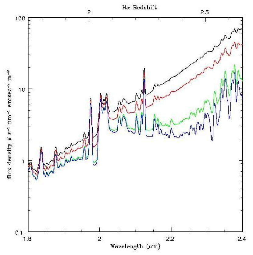
Increasing telescope aperture for an AO-enabled telescope affects the limiting line flux both by increasing the photon collection area and by concentrating the PSF of the diffraction limited image, effectively increasing signal in proportion to the primary mirror diameter $D^{4}$. The net effect as a function of wavelength is shown in Figure 10 for telescopes with $D=5$, 10, 30, and 50 meters. In addition to the improvements in limiting flux, 30-m and larger class telescopes will also permit spatially resolved studies at finer angular scales than possible with current generation instruments since the diffraction limit of a 30-m telescope is $\sim$ 18 mas in the $K$ band (roughly one third that of the Keck telescope).

Figure 11.— As Figure 4, but for a thirty-meter class telescope with an OSIRIS-like IFS.

To illustrate this point we repeat our earlier calculations of the expected S/N ratios for detection of emission from star forming regions using a simulated thirty-meter class telescope (TMT) in combination with an OSIRIS-like spectrograph. As shown in Figure 11, with this configuration even spatially extended sources observed with lenslet sampling scales of 35 mas ($\sim$ 300 pc at redshift $z=2.5$) provide reasonable detections for spectroscopically unresolved emission lines at redshifts up to $z=2.5$ in only an hour of integration. On scales of 100 mas, TMT is likely to provide H$\alpha$ spectra for point-like regions forming stars at a rate of 1 $M_{\odot}$ yr^-1 with a peak S/N ratio of 50+, permitting detailed study of even the fainter components of target galaxies.

4.3. Limiting Line Fluxes: Cryogenic Considerations

As discussed in §3.2 thermal emission dominates the $K$-band background, particularly for large aperture telescopes. This emission comes from telescope primary and secondary mirrors, re-imaging optics in the AO system light path, and atmospheric contributions. Although the latter is uncontrollable for ground-based instruments, it is of obvious interest to attempt to minimize the contribution from optical components (Fig. 12).

Figure 12.— Model effective $K$-band background spectra for: (1) 35% emissivity in AO optics and 20% emissivity in telescope optics at temperature $T=270K$ (black line, as Figure 1), (2) 35% emissivity in AO at $T=270K$ and 0% telescope emissivity (red line), (3) 35% emissivity in AO cryogenically cooled to $T=250K$ and 0% telescope emissivity (green line), (4) 35% emissivity in AO cryogenically cooled to $T=77K$ and 0% telescope emissivity (blue line). All models incorporate the Gemini model for zodiacal light and atmospheric emission, for further commentary see Figure 1.

In Figure 13 we plot the limiting line flux at $K$-band wavelengths for a 30-m class telescope operated under a range of thermal conditions. Assuming it were possible to cryogenically cool the AO bench to $T=-20^{\circ}C$, the thermal emission from the AO system would become largely negligible compared to that from the telescope and atmosphere, pushing the limiting flux in the $K$-band a factor of three lower. If, in addition, it were possible to achieve near-perfect reflectivity from the telescope mirrors, then the combined reduction in background flux would reduce the limiting line flux by a factor of almost ten.

Figure 13.— Limiting line flux density in the $K$-band for a 5$\sigma$ detection in one hour of integration using an OSIRIS-like IFS on a 30-m class telescope (100 mas sampling). Curves are for: (1) 35% emissivity in AO optics and 20% emissivity in telescope optics at temperature $T=270K$ (black line), (2) 35% emissivity in AO at $T=270K$ and 0% telescope emissivity (green line), (3) 35% emissivity in AO cryogenically cooled to $T=250K$ and 20% telescope emissivity at temperature $T=270K$ (blue line), (4) 35% emissivity in AO cryogenically cooled to $T=250K$ and 0% telescope emissivity (red line). Line emission is assumed to be spectrally unresolved.

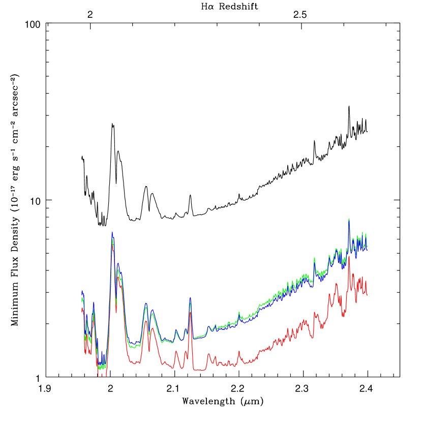
This improvement is most noticeable around wavelengths of 2.2 - 2.4 microns where the atmosphere is particularly transparent, and we therefore gain the most from suppressing emission from optical components. Longward of 2.4 microns however the improvement becomes less pronounced as atmospheric emission begins to increase rapidly.

It is therefore an attractive goal for next-generation telescopes to cryogenically cool their adaptive optics system since a temperature change of only 20 degrees (coupled with increased mirror reflectivity) may suffice to increase sensitivity in the $K$-band by almost an order of magnitude. This 20 degrees of cooling would reduce thermal emission from the AO system to the level of the background sky, so additional cooling (e.g. to liquid nitrogen temperatures $T=77$ K) would not greatly decrease the background further. Such a cooling system should not pose a great technological challenge (C. Max, private communication), although it would somewhat increase the cost and complexity of such a telescope project.

4.4. Spectral Resolution Requirements

Moderate spectral resolution (${\cal R}\sim$ 3000) is necessary for spectroscopic studies of high redshift galaxies, largely so that individual atmospheric OH emission lines may be suppressed, and in general the greater the resolution the greater the range of wavelengths for which it will be possible to achieve inter-line background levels. In addition, high spectral resolution aids in the successful recovery of velocity substructure, and spectrograph resolution must be great enough that it is possible to measure velocities to within tens of km s^-1. We note, however, that the benefits of increasing spectral resolution do not continue indefinitely, but peak when emission lines in a lenslet are just barely unresolved, beyond which detector noise begins to grow as the line emission is spread over a greater number of pixels.

4.5. Benefits of Adaptive Optics

Adaptive optics is a key component for integral-field observations of targets whose angular size is less than or comparable to the size of the seeing disk. Most importantly, AO correction concentrates an appreciable fraction of emitted light into the PSF core of the lenslet subtending the region from which that light was emitted, greatly increasing the signal strength from point sources and permitting improved imaging of structures blurred together in the seeing disk. We note however that for slightly larger sources ($\gtrsim 4$ arcsec²) atmospheric seeing may also be partially corrected for using ground-layer adaptive optics (GLAO) techniques (e.g. Chun 2003) or post-processing wavelet decomposition methods (e.g. Puech et al. 2004, Flores et al. 2004) instead of a conventional adaptive optics system.

One particularly useful observation for which AO correction will be essential is the targeted observation of AGN with integral field spectrographs. In many sources the central AGN often outshines its host galaxy, which may be extremely difficult to study if the AGN emission is blurred over its host in an atmospheric seeing halo. With AO correction however, the AGN emission may be concentrated more fully in its PSF core, decreasing the contamination in the seeing halo and possibly enabling an IFS to probe the emission from, and kinematics of, the host galaxy.

5. SUMMARY

We have outlined an observing strategy for infrared integral-field spectroscopy of high-redshift galaxies, and presented a formalism for simulating observations with an arbitrary telescope plus lenslet spectrograph system. These calculations may be generalized to predict the integration times required to observe extended or compact sources both at high redshift and in the local universe.

We have determined 5$\sigma$ limiting line flux densities as a function of wavelength for typical AO-equipped integral-field spectrographs mounted on telescopes with primary mirror diameters ranging from 5 to 50 meters. Using 100 mas angular sampling, these limiting flux densities are typically $\sim 10^{-16}$ erg s^-1 cm^-2 arcsec^-2 for 10-m class telescopes, and $\sim 10^{-17}$ erg s^-1 cm^-2 arcsec^-2 for 50-m class telescopes. These limiting line fluxes increase by a factor of $\sim$ 3 for each factor of $\sim$ 2 that the angular lenslet scale is decreased. Realistic models of the infrared background flux are taken into account in these calculations, and include blackbody emission from both the atmosphere and telescope optics and atmospheric OH line emission. Warm adaptive optics systems contribute significantly to the $K$-band background flux, and cryogenic cooling to $T=250$ K may reduce the effective background by as much as a factor of ten.

Using parameters characteristic of the Keck/OSIRIS spectrograph we have predicted S/N ratios for detection of line emission from star-forming regions at redshifts $z=0.5-2.5$ with angular lenslet scales of 20, 35, 50, and 100 mas, and find that OSIRIS can observe H$\alpha$ emission from regions forming stars at a rate of about 1 $M_{\odot}$ yr^-1 per 100 mas angular grid square with a signal-to-noise ratio S/N $\sim 10$. Simulated integral-field spectroscopy of $z\sim 2-2.6$ star-forming galaxies in the GOODS-N field indicates that OSIRIS can observe H$\alpha$ emission from these sources with an angular resolution of 100 mas ($\sim$ 1 kiloparsec at redshift $z\sim 2$) and signal-to-noise ratios between 3 and 20, and will be able to produce two-dimensional velocity maps for these galaxies relative to the systemic redshift. These simulated velocity maps suggest that OSIRIS will be able to distinguish between some disparate kinematic models permitted by ambiguous long-slit spectroscopic data alone, and may distinguish between mature disk kinematics and active mergers for spatially extended, bright galaxies at these redshifts.

Further observational constraints on the H$\alpha$ morphologies of the $z\sim 2-2.6$ galaxies from AO-corrected narrow-band photometry will help determine whether sources may resolve into individual star forming regions on scales less than a kiloparsec, permitting more detailed simulations and kinematic studies. The morphological and velocity structure of these galaxies at such small scales may be observable with OSIRIS for particularly bright sources, and will certainly be accessible to future studies using next-generation 30-m and 50-m class telescopes.

References

- Adelberger et al. (2004) Adelberger, K. L., Steidel, C. C., Shapley, A. E., Hunt, M. P., Erb, D. K., Reddy, N. A., & Pettini, M. 2004, ApJ, 607, 226
- Allington-Smith et al. (2004) Allington-Smith, J. R., Dubbeldam, C. M., Content, R., Dunlop, C. J., Robertson, D. J., Elias, J., Rodgers, B., & Turner, J. E. 2004, Proc. SPIE, 5492, 701
- Bacon et al. (1995) Bacon, R., et al. 1995, A&AS, 113, 347
- Bacon et al. (2001) Bacon, R., et al. 2001, MNRAS, 326, 23
- Conselice et al. (2000) Conselice, C. J., Gallagher, J. S., Calzetti, D., Homeier, N., & Kinney, A. 2000, AJ, 119, 79
- Chun (2003) Chun, M. R. 2003, Proc. SPIE, 4839, 94
- Davies et al. (1997) Davies, R. L., et al. 1997, Proc. SPIE, 2871, 1099
- Erb et al. (2003) Erb, D. K., Shapley, A. E., Steidel, C. C., Pettini, M., Adelberger, K. L., Hunt, M. P., Moorwood, A. F. M., & Cuby, J. 2003, ApJ, 591, 101
- Erb et al. (2004) Erb, D. K., Steidel, C. C., Shapley, A. E., Pettini, M., & Adelberger, K. L. 2004, ApJ, 612, 122
- Erb et al. (2005) Erb, D. K., Steidel, C. C., Shapley, A. E., Pettini, M., Reddy, N. A., & Adelberger, K. L. 2005. In preparation.
- Flores et al. (2004) Flores, H., Puech, M., Hammer, F., Garrido, O., & Hernandez, O. 2004, A&A, 420, L31
- García-Lorenzo et al. (2000) García-Lorenzo, B., Arribas, S., & Mediavilla, E. 2000, The Newsletter of the Isaac Newton Group of Telescopes (ING Newsl.), issue no. 3, p. 25-28, 3, 25
- Giavalisco et al. (1996) Giavalisco, M., Steidel, C. C., & Macchetto, F. D. 1996, ApJ, 470, 189
- Giavalisco et al. (2004) Giavalisco, M., et al. 2004, ApJ, 600, L93
- Girardi et al. (2002) Girardi, L., Bertelli, G., Bressan, A., Chiosi, C., Groenewegen, M. A. T., Marigo, P., Salasnich, B., & Weiss, A. 2002, A&A, 391, 195
- Gordon et al. (2004) Gordon, K. D., et al. 2004, ApJS, 154, 215
- Hammer et al. (1999) Hammer, F., Hill, V., & Cayatte, V. 1999, Journal des Astronomes Francais, 60, 19
- Kennicutt (1998) Kennicutt, R. C. 1998, ARA&A, 36, 189
- Kennicutt et al. (2004) Kennicutt, R. C., Lee, J. C., Akiyama, S., Funes, J. G., & Sakai, S. 2004, American Astronomical Society Meeting Abstracts, 205, 6005L
- Larkin et al. (2003) Larkin, J. E., et al. 2003, Proc. SPIE, 4841, 1600
- Lee et al. (2004) Lee, J. C., Kennicutt, R. C., Funes, J. G., Sakai, S., Tremonti, C. A., & van Zee, L. 2004, American Astronomical Society Meeting Abstracts, 205, 6004L
- Lemoine-Busserolle et al. (2003) Lemoine-Busserolle, M., Contini, T., Pelló, R., Le Borgne, J.-F., Kneib, J.-P., & Lidman, C. 2003, A&A, 397, 839
- Lord (1992) Lord, S.D. 1992, NASA Technical Memor. 103957
- McGregor et al. (2003) McGregor, P. J., et al. 2003, Proc. SPIE, 4841, 1581
- Moorwood et al. (2003) Moorwood, A., van der Werf, P., Cuby, J. G., & Oliva, T. 2003, The Mass of Galaxies at Low and High Redshift, 302
- Oke (1964) Oke, J. B. 1964, ApJ, 140, 689
- Papovich et al. (2005) Papovich, C. et al. 2005, ApJ, in press.
- Pettini et al. (2001) Pettini, M., Shapley, A. E., Steidel, C. C., Cuby, J., Dickinson, M., Moorwood, A. F. M., Adelberger, K. L., & Giavalisco, M. 2001, ApJ, 554, 981
- Puech et al. (2004) Puech, M., Flores, H., & Hammer, F. 2004, SF2A-2004: Semaine de l’Astrophysique Francaise.
- Quirrenbach et al. (2003) Quirrenbach, A., Larkin, J. E., Krabbe, A., Barczys, M., & LaFreniere, D. 2003, Proc. SPIE, 4841, 1493
- Ramsay Howat et al. (1998) Ramsay Howat, S. K., et al. 1998, Proc. SPIE, 3354, 456
- Shapley et al. (2001) Shapley, A. E., Steidel, C. C., Adelberger, K. L., Dickinson, M., Giavalisco, M., & Pettini, M. 2001, ApJ, 562, 95
- Steidel et al. (2004) Steidel, C. C., Shapley, A. E., Pettini, M., Adelberger, K. L., Erb, D. K., Reddy, N. A., & Hunt, M. P. 2004, ApJ, 604, 534
- Swinbank et al. (2005a) Swinbank, A. M., Balogh, M. L., Bower, R. G., Hau, G. K. T., Allington-Smith, J. R., Nichol, R. C., & Miller, C. J. 2005a, ApJ, 622, 260
- Swinbank et al. (2005b) Swinbank, A. M., et al. 2005b, MNRAS, 359, 401
- Tecza et al. (1998) Tecza, M., Thatte, N. A., Krabbe, A., & Tacconi-Garman, L. E. 1998, Proc. SPIE, 3354, 394