Scattering of Polarized Radiation by Atoms in Magnetic and Electric Fields

The polarization of radiation by scattering on an atom embedded in combined external quadrupole electric and uniform magnetic fields is studied theoretically. Analytic formulae are derived for the scattering phase matrix. Limiting cases of scattering under Zeeman effect, and Hanle effect in weak magnetic fields are discussed.

1 Introduction

Scattering of polarized radiation by an atom is a topic of considerable interest to astrophysics, especially with the advent of imaging polarimeter systems like ZIMPOL I & II (Gandorfer, 2003) which reach accuracies of the order of $10^{-5}$ for measuring the Stokes parameters characterising the observed radiation. The concept of scattering phase matrix connecting the Stokes vector ${\boldsymbol{\cal S}}^{\prime}$ of incident radiation to the Stokes vector ${\boldsymbol{\cal S}}$ of scattered radiation was introduced quite early in the context of Rayleigh scattering. Landi Degl’Innocenti (1983a, ; 1983b, ; landi-3, 1984, 1985), Landi Degl’Innocenti, Bommier and Sahal-Br$\acute{\rm e}$chot (lbs1, 1990; 1991a, ; 1991b, ) and Bommier (1997a, ; 1997b, ) developed a comprehensive theoretical framework to describe the generation and transfer of polarized radiation in spectral lines, formed in the presence of an external magnetic field. In the context of radiation transfer work, Stenflo and Stenholm (stenflo2, 1976) and Rees (ree, 1978), used complete frequency redistribution (CRD) in the resonance scattering, and Dumont et al. (dumont, 1977), Rees and Saliba (ree2, 1982), Nagendra (nagendra1, 1986, 1988), Faurobert (faur, 1987), Ivanov et al. (ivan, 1997) and later works employed partial frequency redistribution (PRD) line scattering mechanisms in the absence of magnetic field. The Hanle effect is a depolarizing phenomenon which arises due to ‘partially overlapping’ magnetic substates in the presence of weak magnetic fields, where the splitting produced is of the same order as or less than the natural widths. Favati et al. favati (1987) proposed the name ‘second Hanle effect’ for a similar effect in ‘electrostatic fields’. Casini and Landi Degl’Innocenti (casini, 1993) have discussed the problem in the presence of electric and magnetic fields for the particular case of hydrogen lines. The relative contributions of static external electric fields, motional electric fields and magnetic fields in the case of hydrogen Balmer lines, have been studied by Brillant et al. (brillant, 1998). A historical perspective and extensive references to earlier literature on polarized line scattering can be found in Stenflo (stenflo-94, 1994), Trujillo Bueno et al. (tru, 2002) and Landi Degl’Innocenti and Landolfi (ll, 2004). The purpose of this paper is to derive the scattering phase matrix for the case of combined magnetic and electric quadrupole fields with arbitrary strengths. The particular case of transitions between $J=0$ and $J=1$ states is considered following Oo et al.(2004; 2005).

2 Theoretical Formalism

The Hamiltonian for an atom, when it is exposed to an external magnetic field ${\@vec{B}}$ together with an arbitrary external Coulomb field $\Phi$, is of the form (Oo et al., 2004)

$$H=H_{0}+g\,{\@vec{J}}\cdot{\@vec{B}}+\sum^{\infty}_{l=0}\sum^{l}_{m=-l}(-1)^{m}\,V_{lm}\,Q_{l-m}\ ,$$ (1)

where $g$ denotes the gyromagnetic ratio, ${\@vec{J}}$ the total angular momentum operator for the atom with components $J_{x},J_{y},J_{z}$ while $V_{lm}$ denote the $2^{l}$-pole components of $\Phi$ and the components $Q_{l-m}$ characterise the electric charge distribution inside the atom. It is well-known that the magnetic field ${\@vec{B}}$ splits an eigenstate of $H_{0}$ with energy $E$ and total angular momentum quantum number $J$ into $(2J+1)$ equally spaced levels $|J\,M\rangle$ with energies $E_{M}=E+gBM$, where $B=|{\@vec{B}}|$ and $M$ denotes the magnetic quantum number with respect to an axis of quantization chosen along ${\@vec{B}}$. If the atomic states are eigenstates of parity, the $l=1$ term makes no contribution. In an external electric quadrupole field with $l=2$, $V_{2m}$ may equivalently be expressed in terms of the cartesian components $V_{\alpha,\beta}$ with $\alpha,\beta=x,y,z$ of a traceless symmetric second rank tensor, which defines its own Principal Axes Frame (PAF), wherein $V_{\alpha,\beta}=V_{\alpha,\alpha}\,\delta_{\alpha,\beta}$, so that

$$\sum^{2}_{m=-2}(-1)^{m}\,V_{2m}\,Q_{2-m}=A\,\Bigl{[}3J_{z}^{2}-{\@vec{J}}\cdot{\@vec{J}}+\eta\,\{J_{x}^{2}-J_{y}^{2}\}\Bigr{]}\ ,$$ (2)

where $A=Q\,V_{zz}/\{4J(J-1)\}$, if $Q$ denotes the electric quadrupole moment of the atom and $\eta=(V_{xx}-V_{yy})/V_{zz}$ denotes the asymmetry parameter of the field. In such a case, the $(2J+1)$ substates $|\psi_{k}\rangle$ where $k=1,2,\cdots,(2J+1)$ with energies $E_{k}$ are neither equally spaced nor are they identifiable as $|J\,M\rangle$ states. We may, however, represent them as

$$|\psi_{k}\rangle=\sum^{J}_{M=-J}a^{k}_{M}({\@vec{B}},A,\eta)\,|J\,M\rangle\ ,$$ (3)

in terms of $|J\,M\rangle$ states defined with respect to PAF, where the expansion coefficients $a^{k}_{M}$ as well as the energies $E_{k}$ are not only functions of $B,A,\eta$ but also of the angles $(\widetilde{\theta}_{B},\widetilde{\phi}_{B})$ of ${\@vec{B}}$ with respect to PAF (see Fig. 1). For a detailed discussion for $J=1,\frac{3}{2}$ (see Oo et al. 2004; 2005).

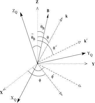
Figure 1: The scattering geometry: $({\rm X}_{Q},{\rm Y}_{Q},{\rm Z}_{Q})$ refers to the Principal Axes Frame (PAF) characterising the electric quadrupole field. The radiation is incident along $(\theta^{\prime},\phi^{\prime})$ and scattered along $(\theta,\phi)$ with respect to the astrophysical reference frame denoted by $({\rm X},{\rm Y},{\rm Z})$. The magnetic field ${\@vec{B}}$ is oriented along $(\widetilde{\theta}_{B},\widetilde{\phi}_{B})$ with reference to PAF and $(\theta_{B},\phi_{B})$ with reference to the astrophysical reference frame (the azimuthal angles $\widetilde{\phi}_{B}$ and $\phi_{B}$ are not marked in the figure).

The PAF itself may, in general, be different from the astrophysical frame, in which case

$$|\psi_{k}\rangle =\sum^{J}_{m=-J}c^{k}_{m}\,|J\,m\rangle\ ; k =1,2,\cdots,(2J+1)\ ,$$ (4)

in terms of the $|J\,m\rangle$ states defined with respect to the astrophysical frame and

$$c^{k}_{m}=\sum^{J}_{M=-J}a^{k}_{M}({\@vec{B}},A,\eta)\,D^{J}_{mM}(\alpha_{Q},\beta_{Q},\gamma_{Q})\ ,$$ (5)

if $(\alpha_{Q},\beta_{Q},\gamma_{Q})$ denote the Euler angles of the PAF with respect to the astrophysical frame. If the magnetic field alone is present, $|\psi_{k}\rangle$ are identical with $|J\,M\rangle$ states and $c^{M}_{m}=D^{J}_{mM}(\phi_{B},\theta_{B},0)$ in Eq. (4).

We now consider the scattering of polarized radiation by an atom which makes a transition from an initial state $|\psi_{i}\rangle$ with energy $E_{i}$, total angular momentum $J_{i}$ and parity $\pi_{i}$ to a final state $|\psi_{f}\rangle$ with energy $E_{f}$, total angular momentum $J_{f}$ and parity $\pi_{f}$ when polarized radiation with frequency $\nu^{\prime}$ is incident on the atom in the astrophysical frame in a direction $(\theta^{\prime},\phi^{\prime})$ and gets scattered into a direction $(\theta,\phi)$ with frequrncy $\nu$. The left and right circular states of polarization as defined by Rose (rose, 1957) are denoted by $\mu=\pm 1$. The second order transition matrix element for scattering of polarized radiation may then be written, with respect to the polarization states as

$$T_{\mu\mu^{\prime}}=\sum_{n}{\cal E}_{fn}(\mu)\,\Phi_{n}\,{\cal A}_{ni}(\mu^{\prime})\ ,$$ (6)

where the summation is with respect to the intermediate states $|\psi_{n}\rangle$ of the atom with energy $E_{n}$, total angular momentum $J_{n}$ and parity $\pi_{n}$. Following (Oo et al., 2004), the matrix elements for emission from $|J_{u}\,m_{u}\rangle$ to $|J_{l}\,m_{l}\rangle$ are of the form

$${\cal E}_{m_{l}m_{u}}(\mu) = \sum_{L}{\cal J}_{L}\,\sum^{L}_{M_{L}=-L}C(J_{l},L,J_{u};m_{l},M_{L},m_{u})\,$$ (7)

$$D^{L}_{M_{L}\mu}(\phi,\theta,0)^{*}\ ,$$

where ${\cal J}_{L}$ is proportional to the reduced matrix element. The complex conjugate of Eq. (7) defines the matrix elements ${\cal A}_{m_{u}m_{l}}(\mu)$ for absorption of radiation with polarization $\mu$ incident along $(\theta,\phi)$ leading to $|J_{u}\,m_{u}\rangle$ from $|J_{l}\,m_{l}\rangle$. Using the notations $\omega=2\pi\nu;\ \ \omega^{\prime}=2\pi\nu^{\prime}$;  $\omega_{n}=E_{n}-E_{f}$ and $\omega^{\prime}_{n}=E_{n}-E_{i}$, the profile function $\Phi_{n}=(\omega_{n}-\omega-{\rm i}\Gamma_{n})^{-1}=(\omega^{\prime}_{n}-\omega^{\prime}-{\rm i}\Gamma_{n})^{-1}$ where the width associated with $|\psi_{n}\rangle$ is denoted by $\Gamma_{n}$ and energy conservation requires $E_{i}+\omega^{\prime}=E_{f}+\omega$. Angular momentum and parity are conserved individually during the absorption and the emission.

3 Scattering Phase Matrix

If ${\boldsymbol{\cal S}}^{\prime}$ denotes the Stokes vector, which characterizes the state of polarization of the incident radiation, the Stokes vector ${\boldsymbol{\cal S}}$ characterizing the scattered radiation is

$${\boldsymbol{\cal S}}={\cal R}\ \ {\boldsymbol{\cal S}^{\prime}}\ ,$$ (8)

where ${\cal R}$ is a $(4\times 4)$ matrix whose elements are of the form

$${\cal R}_{pp^{\prime}}=\sum_{nn^{\prime}}\Phi_{n}\,\Phi^{*}_{n^{\prime}}\,{\cal P}^{nn^{\prime}}_{pp^{\prime}}\ ,$$ (9)

where the phase matrix elements are given by

$${\cal P}^{nn^{\prime}}_{pp^{\prime}}=\frac{1}{2}\sum_{\mu,\mu^{\prime}\atop\mu^{\prime\prime},\mu^{\prime\prime\prime}}{(\sigma^{\gamma}_{p^{\prime}})}_{\mu^{\prime}\mu^{\prime\prime\prime}}\,{(\sigma^{\gamma}_{p})}_{\mu^{\prime\prime}\mu}\,$$

$$Tr\Bigl{[}{\cal E}(\mu)\,{\cal C}^{n}\,{\cal A}(\mu^{\prime})\,{\cal C}^{i}\,{\cal A}^{{\dagger}}(\mu^{\prime\prime\prime})\,{\cal C}^{n^{\prime}}\,{\cal E}^{{\dagger}}(\mu^{\prime\prime})\,{\cal C}^{f}\Bigr{]}\ ,$$ (10)

with $p,p^{\prime}=0,1,2,3$, using the density matrix formalism (McMaster, 1961) for polarization of radiation. The $\sigma^{\gamma}_{p}$ with $p=1,2,3$ are Pauli matrices with respect to basis states $\mu=\pm 1$ for radiation, while $\sigma^{\gamma}_{0}=1$. We use the notation $Tr(\equiv\sum_{m_{f}})$ to denote the Trace of the $(2J_{f}+1)\times(2J_{f}+1)$ matrix contained within the square bracket. The ${\cal C}^{i},{\cal C}^{f},{\cal C}^{n}$ and ${\cal C}^{n^{\prime}}$ are defined in terms of their elements

$${\cal C}^{i}_{m_{i}m^{\prime}_{i}} =c^{i}_{m_{i}}\,c^{i^{*}}_{m^{\prime}_{i}}\ ; {\cal C}^{f}_{m_{f}m^{\prime}_{f}} =c^{f}_{m_{f}}\,c^{f^{*}}_{m^{\prime}_{f}}\ ,$$

$${\cal C}^{n}_{m_{n}m^{\prime}_{n}} =c^{n}_{m_{n}}\,c^{n^{*}}_{m^{\prime}_{n}}\ ; {\cal C}^{n^{\prime}}_{m_{n^{\prime}}m^{\prime}_{n^{\prime}}} =c^{n^{\prime}}_{m_{n^{\prime}}}\,c^{{n^{\prime}}^{*}}_{m^{\prime}_{n^{\prime}}}\ .$$ (11)

Each of these matrices ${\cal C}^{i},{\cal C}^{f},{\cal C}^{n},{\cal C}^{n^{\prime}}$ are clearly hermitian and satisfy the condition ${\cal C}^{2}={\cal C}$. Note that the ${\cal P}^{nn^{\prime}}_{pp^{\prime}}$ depend not only on $n$ and $n^{\prime}$ but also on the direction $(\widetilde{\theta}_{B},\widetilde{\phi}_{B})$ and the strength $B$ of the magnetic field ${\@vec{B}}$ and on $(A,\eta;\alpha_{Q},\beta_{Q},\gamma_{Q})$ characterising the electric quadrupole field (because of Eq. (4) for the $c^{k}_{m}$ with $k=i,f,n,n^{\prime}$), apart from the angles $(\theta^{\prime},\phi^{\prime})$ of the incident and $(\theta,\phi)$ of the scattered radiation. Explicitly, therefore, ${\cal P}^{nn^{\prime}}_{pp^{\prime}}\equiv{\cal P}^{nn^{\prime}}_{pp^{\prime}}(\theta,\phi;\theta^{\prime}\phi^{\prime};{\@vec{B}};A,\eta;\alpha_{Q},\beta_{Q},\gamma_{Q})$ for any given $J_{i},J_{f}$. In the case of resonance scattering, when only a single intermediate state $|\psi_{n}\rangle$ with $E_{n}=E_{i}+\omega^{\prime}=E_{f}+\omega$ contributes to Eq. (6), one can replace the summation over $n,n^{\prime}$ by $n=n^{\prime}$ corresponding to a single excited level, whereas the double summation over $n,n^{\prime}$ has to be retained in Hanle scattering.

4 Particular Case

We consider the simple case of scattering with electric dipole transitions between a total angular momentum zero lower level and a total angular momentum one upper level, i.e., $J_{l}=J_{i}=J_{f}=0$ and $J_{u}=J_{n}=1$. Clearly, ${\cal C}^{i}={\cal C}^{f}=1$. We may then use Eq. (7) to simplify the product ${\cal E}^{{\dagger}}(\mu^{\prime\prime})\,{\cal E}(\mu)$ and use the complex conjugate of Eq. (7) to simplify the product ${\cal A}(\mu^{\prime})\,{\cal A}^{{\dagger}}(\mu^{\prime\prime\prime})$ in Eq. (10), so that

$${\cal P}^{nn^{\prime}}_{pp^{\prime}} =\frac{1}{2}\,g^{nn^{\prime}}_{p}(\theta,\phi)\,g^{nn^{\prime}}_{p^{\prime}}(\theta^{\prime},\phi^{\prime})^{*}\ ; n,n^{\prime} =1,2,3\ ,$$ (12)

in terms of

$$g^{nn^{\prime}}_{p}(\theta,\phi)=|{\cal J}_{1}|^{2}\sum^{2}_{\lambda=0}\sum^{1}_{m^{\prime},m^{\prime\prime}=-1}C(1,1,\lambda;m^{\prime},-m^{\prime\prime},m)$$

$$(-1)^{m^{\prime\prime}}\sum^{\lambda}_{\xi=-\lambda}f_{p}(\lambda,\xi)\,D^{\lambda}_{m\xi}(\phi,\theta,0)\,c^{n}_{m^{\prime\prime}}\,c^{{n^{\prime}}^{*}}_{m^{\prime}}\ ,$$ (13)

where

$$f_{0}(\lambda,\xi) = \frac{2}{\sqrt{3}}\,\delta_{\xi,0}\Bigl{[}\delta_{\lambda,0}+\frac{1}{\sqrt{2}}\,\delta_{\lambda,2}\Bigr{]}\ ,$$

$$f_{1}(\lambda,\xi) = -\delta_{\lambda,2}\Bigl{[}\delta_{\xi,2}+\delta_{\xi,-2}\Bigr{]}\ ,$$

$$f_{2}(\lambda,\xi) = {\rm i}\,\delta_{\lambda,2}\Bigl{[}\delta_{\xi,2}-\delta_{\xi,-2}\Bigr{]}\ ,$$

$$f_{3}(\lambda,\xi) = \sqrt{2}\,\delta_{\xi,0}\,\delta_{\lambda,1}\ .$$ (14)

In the absence of the electric field, $n=M,n^{\prime}=M^{\prime}$ and the $c^{M}_{m}=D^{1}_{mM}(\phi_{B},\theta_{B},0)$, leading to the well-known Hanle scattering phase matrix given by Eqs. (9) to (16) of Landi and Landi (2landi, 1988) if $\Phi_{M}\Phi^{*}_{M^{\prime}}$ can be assumed to be independent of $M,M^{\prime}$ in the limiting case of weak fields. If the Doppler convolution is effected following exactly the procedure outlined by Stenflo (1998), the Hanle-Zeeman scattering matrix represented by Eqs. (49) and (50) of Stenflo (1998) is recovered for $\theta_{B}=\phi_{B}=0$. In the case of strong fields i.e, if $g\,B$ is large compared to the line widths (Zeeman effect), one may set $M=M^{\prime}$ and recover Eq. (52) of Stenflo (1998) for $\theta_{B}=\phi_{B}=0$ and the results obtained much earlier by Obridko 1965a .

5 Numerical Results and Discussion

If we consider the simplest geometry of the combined magnetic and quadrupole electric fields with ${\@vec{B}}$ along the ${\rm Z}$-axis of the PAF with the PAF itself coinciding with the astrophysical frame i.e., $\alpha_{Q}=\beta_{Q}=\gamma_{Q}=\widetilde{\theta}_{B}=\widetilde{\phi}_{B}=\theta_{B}=\phi_{B}=0$, the upper level with $J_{u}=1$ is split into three levels $n=1,2,3$ (Oo et al., 2004) with energies

$$E_{1} =-2\,r\,g\,B\ ; E_{2,3} =(r\mp s)g\,B\ ,$$ (15)

where $r=A/gB$ the ratio of the electric quadrupole and magnetic field strengths, $s=(r^{2}\eta^{2}+1)^{1/2}$ and the corresponding eigen states $|\psi_{1}\rangle,|\psi_{2}\rangle$ and $|\psi_{3}\rangle$ characterized by

$$c^{1}_{0} = 1,\ \ \ c^{1}_{\pm 1}=c^{2,3}_{0}=0$$

$$c^{3}_{\pm 1} = \pm c^{2}_{\mp 1}=(s+r\,\eta\pm 1)/2(s^{2}+r\,\eta\,s)^{1/2}\ ,$$ (16)

using Eqs. (4) and (5), with the electric quadrupole field strength $A>0$.

To understand the combined effect of magnetic and electric quadrupole fields, we present in Figs. (2d-2f) the general behavior of the scattered Stokes line profiles ${\boldsymbol{\cal S}}$ for a given unpolarized incident radiation, ${\boldsymbol{\cal S}^{\prime}}=(1\ 0\ 0\ 0)^{T}$, for particular choices of the directions $(\theta^{\prime}=\frac{\pi}{4},\phi^{\prime}=0)$ and $(\theta=\frac{\pi}{4},\phi=\pi)$. We compare these with the pure Zeeman scattering case (see Figs. 2a-2c). In the Stokes $Q$ profile, the positive maximum at the line center and the negative maximum symmetrically placed at $\sigma_{\pm 1}$ components, which are typical of the well known Zeeman effect. The maximum of the $V$ profile at $\sigma_{\pm 1}$ components have opposite sign, which is also a well known characterisitc of Zeeman effect. We assume here that the magnetic field and the quadrupole electric field are equally strong (i.e., $r=A/B=1$). We also assume $B$ to be four times the natural line width and set $n=n^{\prime}=1,2,3$. The solid and dashed curves in Figs. (2d-2f) are computed for the values of $\eta=0$ and $1$ respectively. In the combined fields case, the line component arising due to the $|\psi_{1}\rangle=|1,0\rangle$ state (which represents the central component in the corresponding pure Zeeman case) is positioned in the red wing (see Figs. 2d-2f). The unequal strengths of the scattered line profiles arising from $|\psi_{2}\rangle$ and $|\psi_{3}\rangle$ states are clearly seen in all the scattered Stokes line profiles $(I,Q,V)$. This is due to the weighted superposition of the magnetic substates $|1,-1\rangle$ and $|1,1\rangle$. In the scattered Stokes $V$ line profile, $|\psi_{1}\rangle$ state does not contribute, as in the case of pure Zeeman scattering. Therefore the shape of the scattered Stokes $V$ profile is similar to the Zeeman case, except for the shifting of the position and the change in the relative strength of components when $\eta>0$. If $\eta$ vanishes, the strengths of both components are same.

Figure 2: Stokes line profiles in arbitrary units comparing the Zeeman scattering in a pure magnetic field (panels ${\bf a}-{\bf c}$), and scattering under the combined magnetic and electric quadrupole fields (panels ${\bf d}-{\bf f}$) with $r=1$. The solid lines correspond to asymmetry parameter $\eta=0$, and the dashed lines to $\eta=1$. In all panels, ${\it x}$ is the frequency displacement from the line center in natural width units.

References

- (1) Bommier, V. 1997a, A&A, 328, 706
- (2) Bommier, V. 1997b, A&A, 328, 726
- (3) Brillant, S., Mathys, G., & Stehle, C. 1998, A&A, 339, 286
- (4) Casini, R., & Landi Degl’Innocenti, E. 1993, A&A, 276, 289
- (5) Dumont, S., Pecker, J. C., Omont, A., & Rees, D. E. 1977, A&A, 54, 675
- (6) Favati, B., Landi Degl’Innocenti, E., Landolfi, M. 1987, A&A, 179, 329
- (7) Faurobert, M. 1987, A&A, 178, 269
- Gandorfer (2003) Gandorfer, A. M. 2003, Astron. Nachr./AN, 324, 318
- (9) Ivanov, V. V., Grachev, S. I., & Loskutov, V. M. 1997, A&A, 318, 315
- (10) Landi Degl’Innocenti, E. 1983a, Solar Phys, 85, 3
- (11) Landi Degl’Innocenti, E. 1983b, Solar Phys, 85, 33
- (12) Landi Degl’Innocenti, E. 1984, Solar Phys, 91, 1
- (13) Landi Degl’Innocenti, E. 1985, Solar Phys, 102, 1
- (14) Landi Degl’Innocenti, M., & Landi Degl’Innocenti, E. 1988, A&A, 192, 374
- (15) Landi Degl’Innocenti, E., Bommier, V., & Sahal-Brshot, S. 1990, A&A, 235, 459
- (16) Landi Degl’Innocenti, E., Bommier, V., & Sahal-Brchot, S. 1991a, A&A, 244, 391
- (17) Landi Degl’Innocenti, E., Bommier, V., & Sahal-Brchot, S. 1991b, A&A, 244, 401
- (18) Landi Degl’Innocenti, E., & Landolfi, M. 2004, Polarization in Spectral Lines, Kluwer, Netherlands
- McMaster (1961) McMaster, W. H. 1961, Rev. Mod. Phys., 33, 8
- (20) Nagendra, K. N. 1986, Ph. D. Thesis, Bangalore University, India
- (21) Nagendra, K. N. 1988, ApJ, 335, 269
- (22) Obridko, V. N. 1965a, Soviet Physics-Astronomy, 9, 77
- (23) Rees, D. E. Publ. Astron. Soc. Japan, 1978, 30, 455
- (24) Rees, D. E. & Saliba, G. J. 1982, A&A, 115, 1
- (25) Rose, M. E., 1957, Elementary Theory of Angular Momentum, John Willy, New York
- (26) Stenflo, J. O., & Stenholm, L. 1976, A&A, 46, 69
- (27) Stenflo, J. O. 1994, Solar Magnetic Fields- Polarized Radiation Diagnostics, Kluwer, Dordrecht
- (28) Stenflo, J. O. 1998, A&A, 338, 301
- (29) Trujillo Bueno, J., Moreno Insertis, F., Snchez, F. (Eds.) 2002, Astrophysical Spectropolarimetry, Cambridge Univ. Press, Cambridge
- Oo et al. (2004) Yee Yee Oo, Nagendra, K. N., Sharath Ananthamurthy, Vijayshankar, R., & Ramachandran, G. 2004, J. Quant. Spec. Radiat. Transf., 84, 35
- (31) Yee Yee Oo, Nagendra, K. N., Sharath Ananthamurthy, Swarnamala Sirsi, Vijayshankar, R., & Ramachandran, G. 2005, J. Quant. Spec. Radiat. Transf., 90, 343