Template fitting and the large-angle CMB anomalies

Abstract

We investigate two possible explanations for the large-angle anomalies in the Cosmic Microwave Background (CMB): an intrinsically anisotropic model and an inhomogeneous model. We take as an example of the former a Bianchi model (which leaves a spiral pattern in the sky) and of the latter a background model that already contains a non-linear long-wavelength plane wave (leaving a stripy pattern in the sky). We make use of an adaptation of the “template” formalism, previously designed to detect galactic foregrounds, to recognize these patterns and produce confidence levels for their detection. The “corrected” maps, from which these patterns have been removed, are free of anomalies, in particular their quadrupole and octupole are not planar and their intensities not low. We stress that although the “template” detections are not found to be statistically significant they do correct statistically significant anomalies.

I Introduction

Since the release of the first year data from NASA’s Wilkinson Microwave Anisotropy Probe (wmap, ) there have been extensive studies of the Cosmic Microwave Background (CMB) maps. Generally the results impressively support the favoured $\Lambda$CDM cosmological model, though a lack of power on the largest scales has produced much debate (see e.g., efstat ; bridle ; biel ; contaldi ; teg ; riaz ; slosar2 ). Of further interest are studies that have detected evidence for significant departures from the fundamental cosmological assumption that the universe is isotropic and homogeneous (hbg, ; erik1, ; erik3, ; teg, ; vielva, ; copilet, ; evil, ; dodec, ; ral, ; us, ; tesse, ; hansen, ). Thus it appears the large angle CMB multipoles are anomalous in two seemingly distinct ways. Firstly their power $C_{\ell}$ is abnormally low. Secondly they have an improbable directionality revealed by the fact that for a certain $z$-axis’ orientation one $m$-mode absorbs most of the power, for $\ell=2,...,5$ (evil, ). Naively one may expect the two features to be related: the absence of power in all possible $m$ modes may be why the observed average $C_{\ell}$ is so low. But this has to be made rigorous. Such is the purpose of this letter: could it be that accounting for the large-angle directional multipoles accounts for the observed low $C_{\ell}$?

$\Lambda$CDM theory matches the power spectrum very well on most scales (wmap, ), but the strong non-Gaussianity and/or anisotropy of the low multipoles suggests a competition between two processes: Gaussian isotropic random fluctuations and a deterministic process. One possibility for the latter is intrinsic cosmic anisotropy (as encoded in the Bianchi models) which imparts a spiral pattern in the CMB as studied in barrow ; pedro ; kogut ; tesse . Another is a background model that already contains a non-linear long-wavelength plane wave. This would leave a striking stripy pattern in the sky (a “Jupiter”, if the polar axis is defined suitably). The matter may then be addressed by regarding these patterns as a “contamination” template, and attempting to “correct” the data for its coupling to the template, thereby purifying the underlying Gaussian process. The formalism has been developed to deal with galactic foregrounds but may be adapted to this situation.

We therefore seek a template capable of explaining the preferred axis in the CMB, and ask the question: could the corrected map reveal higher $C_{\ell}$s, thus linking the two issues? Note that this is highly non-trivial. Usually when one corrects a map for a “foreground” the power in the corrected map is smaller. However it could also be that the deterministic process acted destructively. For this to be possible the template would have to have a pattern complementary to the observed data, i.e., contain power in (at least some of the) $m$s which fail to reveal it in the data; in addition this power would have to have acted destructively upon the underlying Gaussian process, so that only one $m$ mode survived in the data.

The presence of a template is more likely to add power than to remove it, so to explain the low-$\ell$ low power this way one relies in part on a chance alignment of phases between the Gaussian fluctuations and the template. Still, in this paper we explore this approach with two different models. In both cases, once we correct the data, and are left with a map with higher low-multipole power $C_{\ell}$, and no preferred direction as seen in evil .

In Section II we outline our method for selecting favoured templates. Then in III we introduce the templates of our two specific models, and in Section IV we explain how we selected the data and record our results. We discuss the implications of these in Sections V and VI.

II The Formalism

Our work is modelled on that of tesse but with an important extension. We start by reviewing tesse . Suppose the sky ${\mathbf{d}}$ may be modelled as the sum of a Gaussian process ${\mathbf{g}}$ and a non-Gaussian “template”, ${\mathbf{t}}$. Then the Maximum Likelihood Estimation (MLE) problem may be set up by introducing a coupling parameter $\alpha$ so that ${\mathbf{d}}={\mathbf{g}}+\alpha{\mathbf{t}}$. The usual MLE problem now concerns ${\mathbf{d}}-\alpha{\mathbf{t}}$, that is:

$$-2\ln{\cal L} = \chi^{2}+\ln\det{\mathbf{M}}$$ (1)

$$\chi^{2} = ({\mathbf{d}}-\alpha{\mathbf{t}})^{\rm T}{\mathbf{M}}^{-1}({\mathbf{d}}-\alpha{\mathbf{t}})$$ (2)

(we have ignored an additive constant in the first expression). Here ${\mathbf{M}}$ is the covariance matrix of ${\mathbf{g}}$ (which may include noise) and the data vectors may be either temperatures in pixel space, or a set of spherical harmonic coefficients $a_{\ell m}$. In the latter case the data is complex, satisfying “reality” constraints; the concomitant modifications to the formalism are trivial. For full sky maps the $a_{\ell m}$ are the preferred formulation.

In general we have a joint estimation problem for $\alpha$ and the unknowns parameterizing ${\mathbf{M}}$ (which can be binned $C_{\ell}$ or the half-dozen parameters encoding “cosmic concordance”). However it is often the case that the range of $\ell$s which decides the ${\mathbf{M}}$ problem and that for the template are disjoint. For example the geometry of the Universe $\Omega$, or the amount of baryonic matter $\Omega_{b}$ are mainly decided by the Doppler peaks, whereas we are interested in templates producing large-angle non-Gaussian features (say $\ell=2-5$; see evil ). One may then decouple the two problems: find ${\mathbf{M}}$ ignoring the template and then solve for $\alpha$ using this solution for ${\mathbf{M}}$.

II.1 Parameter Estimation

The MLE problem for $\alpha$ then becomes the problem of minimizing $\chi^{2}$. The solution is

$$\alpha_{min}={{\mathbf{t}}^{\rm T}{\mathbf{M}}^{-1}{\mathbf{d}}\over{\mathbf{t}}^{\rm T}{\mathbf{M}}^{-1}{\mathbf{t}}}$$ (3)

By construction $\alpha$ is a Gaussian variable. Its variance is

$$\delta\alpha^{2}={1\over{\mathbf{t}}^{\rm T}{\mathbf{M}}^{-1}{\mathbf{t}}}$$ (4)

Two comments are in order. Firstly notice that this formalism wants the template to be like the data. If a mysterious theory was found predicting ${\mathbf{t}}={\mathbf{d}}$, then $\alpha=1$ and the MLE problem tells us that the Gaussian process is in fact absent . This is not in line with common sense: we do know that there is a Gaussian process. Secondly this procedure always produces a corrected map ${\mathbf{d}}-\alpha{\mathbf{t}}$ with lower chi-squared than the original map ${\mathbf{d}}$. This is fine if one suspects contamination because of an abnormally high chi-squared, but what if the observed chi-squared is too low? In that case the corrected map is even more abnormal.

As is usually the case, these quibbles boil down to the choice of parameters and priors used. We have failed to impose a suitable condition enforcing the presence of a Gaussian process, so that the corrected maps have a reduced chi-squared close to 1. If we are in $a_{\ell m}$ space, for example, we are assuming a uniform prior in $a_{\ell m}$. The peak of the distribution is always at $a_{\ell m}=0$, so if ${\mathbf{t}}$ is such that this condition can be satisfied that is precisely what the formalism does (a zero chi-squared is the highest probability configuration if one assumes uniform priors in $a_{\ell m}$). Seen in another way, if we have a deterministic template competing with a Gaussian process on equal footing, the formalism will always try to suppress the random Gaussian process in favour of the certainties of the template.

To address this issue we use an alternative function of the data in calculating the likelihood. We base the likelihood on the probability distribution of the $\ln(\chi^{2})$ (this rather than $\chi^{2}$ produces the correct power spectrum estimator). By changing variables the likelihood is given by

$$-2\ln{\cal L}=\chi^{2}+\ln\det{\mathbf{M}}+D\ln(\chi^{2})$$ (5)

where $D$ is the number of degrees of freedom (i.e. the number of pixels, or the number of $a_{\ell m}$ being considered). Its maximization with respect to $\alpha$ now leads to:

$${\partial\chi^{2}\over\partial\alpha}{\left({D\over\chi^{2}}-1\right)}=0$$ (6)

i.e. either the first factor is zero (equivalent to the problem of minimizing the $\chi^{2}$ solved above), or $\chi^{2}=D$, which means the reduced chi-squared is 1. This is simple to solve, and involves finding the roots to the quadratic equation (2). The solution is

$$\alpha_{\pm}={\chi^{2}_{dt}\pm{\sqrt{\chi^{4}_{dt}-\chi^{2}_{t}(\chi^{2}_{d}-D)}}\over\chi^{2}_{t}}$$ (7)

where

$$\chi^{2}_{t} = {\mathbf{t}}^{\rm T}{\mathbf{M}}^{-1}{\mathbf{t}}$$ (8)

$$\chi^{2}_{d} = {\mathbf{d}}^{\rm T}{\mathbf{M}}^{-1}{\mathbf{d}}$$ (9)

$$\chi^{2}_{dt} = {\mathbf{t}}^{\rm T}{\mathbf{M}}^{-1}{\mathbf{d}}$$ (10)

This formalism for correcting the map generalizes that of tesse , while reducing to it in the appropriate circumstances. If the quadratic does not have real solutions for $\alpha$ (because the minimum of $\chi^{2}(\alpha)$ is above $D$) then the problem reduces to tesse . This is the case where the chi-squared of the data is too high, so that correcting it entails reducing it. In this case the two formalisms agree. However if the data’s chi-squared is too low then our formalism takes over. The quadratic then has real solutions, and the MLE problem is solved by solutions $\alpha_{\pm}$ given by (7).

We note that this approach could be conceptually improved by factorizing the likelihood $\ell$ by $\ell$ and imposing uniform priors on an appropriate function of each $\chi^{2}_{\ell}$. Minimising the likelihood with respect to $\alpha$ would now lead to the problem of solving

$$\sum_{\ell}{\partial\chi^{2}_{\ell}\over\partial\alpha}{\left({D\over\chi^{2}_{\ell}}-1\right)}=0$$ (11)

However, this is in practice impossible to solve, especially for large $\ell_{\rm max}$. Therefore, we are solving for the simpler case of $\chi^{2}=\sum_{\ell}\chi^{2}_{\ell}$.

II.2 Model Comparison

We have found the necessary correction to make for a given template. Perhaps more important is to find the preferred template - i.e., the preferred model. The Bayesian approach to model comparison is to marginalise over the parameters of a model, to find the probability of data given the model (whatever the parameters), as this relates to the probability of the model given the data. We have been working with $P(\alpha,t)$, and above we discuss the specific $\alpha$ solutions that maximise this for a given template. We now wish to compare the likelihood of different templates, that is we require just $P(t)$ - a marginalization over $\alpha$. The standard approach to this (see for e.g AJ ; slosar ) is to absorb the uncertainties of $\alpha$ into the covariance matrix. That is

$$\chi^{2}={\mathbf{d}}^{\mathbf{T}}{\mathbf{M}^{\prime}}^{-1}{\mathbf{d}}$$ (12)

for

$${\mathbf{M}^{\prime}}^{-1}=\lim_{\sigma\to\infty}({\mathbf{M}}+\sigma^{2}{\mathbf{t}}^{\mathbf{T}}{\mathbf{t}})^{-1}$$ (13)

where ${\mathbf{M}}$ is the usual covariance matrix associated with the $a_{\ell m}$s as used above. Using the Sherman-Morrison-Woodbury (AJ, ) formula we find

$${\mathbf{M}^{\prime}}^{-1}={\mathbf{M}}^{-1}-{\mathbf{M}}^{-1}{\mathbf{t}}({\mathbf{t}}^{\mathbf{T}}{\mathbf{M}}^{-1}{\mathbf{t}}){\mathbf{t}}^{\mathbf{T}}{\mathbf{M}}^{-1}$$ (14)

and therefore

$$\chi^{2}=\chi^{2}_{d}-\frac{(\chi^{2}_{dt})^{2}}{\chi^{2}_{t}}\equiv\chi^{2}_{d}-\Gamma^{2}$$ (15)

Assuming uniform priors on our templates, our model comparison now involves maximising the likelihood (5) using the new expression for $\chi^{2}$ and the matrix ${\mathbf{M}^{\prime}}$. In slosar there is a discussion of how this method of marginalising over $\alpha$ inside the covariance matrix is equivalent to ignoring the data that correlates with the template when working out the $\chi^{2}$.

The likelihood function (5) has its maximum at $\chi^{2}=D$. The effective chi-squared from a template is given by Eq. (15) and we see it is always less than $\chi^{2}_{d}$. Therefore, if the initial chi-squared of the data is low: $\chi^{2}<\chi^{2}_{d}<D$, the preferred template is that which maximises the $\chi^{2}$ (minimises $\Gamma$) so as to bring it as close to $\chi^{2}_{d}$ as possible, the optimal solution being $\Gamma=0$. Conversely, if the data has a high chi-squared our formalism reduces to that of tesse , where we maximise $\Gamma$ so as to reduce the $\chi^{2}$ to as close to D as possible.

III The Templates

We consider two prototypes of violation of isotropy and homogeneity: Bianchi models and plane-wave inhomogeneous models.

III.1 Bianchi models

Bianchi models are well-known homogeneous, anisotropic generalizations of Friedmann-Robertson-Walker models. They may be used as a competitor to standard cosmology, constraining violations of isotropy while still assuming homogeneity. In these models the CMB is never isotropic, even before fluctuations are added on. Of particular interest are Bianchi $VII_{h}$ models, for which an asymmetric spiral pattern is imprinted upon the sky. These models were extensively examined in tesse with reference to asymmetries in the power spectrum and anomalous hot-spots. We have reproduced these results with our programs. One of the deficiencies of the fits found in tesse (recognized by the authors) is that they require $\Omega\neq 1$. This would almost certainly lead to a bad fit at high $\ell$ even if the large-angle corrected map is improved. For this reason here we shall restrict ourselves to $\Omega=1$ models.

We follow the parametrisation of the Bianchi $VII_{h}$ model from barrow . These parameters are $\Omega$, $x=\sqrt{h/(1-\Omega)}$, handedness, and the Euler angles $(\phi,\theta,\psi)$. We refer the reader to barrow for a fuller explanation. We fit templates with $\Omega=1$, and explore the range $x\in[0.1,10]$, with both left and right handedness, over the total range of Euler angles.

III.2 Plane-wave cosmology

Inhomogeneous cosmologies are either very simple or very complicated inhom . We consider a model in which a plane wave in the gravitational potential $\Phi$ is part and parcel of the background model (i.e. the unperturbed, zeroth order cosmological model, before the standard Gaussian isotropic scale-invariant adiabatic fluctuations are added to it).

An outstanding wave might be the result of several processes. It could be for example the hallmark of non-trivial topology gomero ; dodec ; riaz . Non-trivial topologies may be ruled out on the grounds that they would imprint repeat patterns in the CMB sky, e.g. matching circles in antipodal locations for the most basic “slab topology”. This constraint is only applicable if the fundamental domain is smaller than the last scattering surface.

Larger-than-the-horizon domains have two effects upon the density plane waves riding the homogeneous model. Firstly modes must fit into the domain, leading to a discretization. But they also introduce a scale in the problem, the size of the domain, $L$. Hence the usual naive arguments for scale-invariance no longer apply and $k^{3}\Phi^{2}$ may actually be a function of $kL$ without introducing an arbitrary scale in the problem. We speculate that even if $L$ is sufficiently large that one may neglect mode discretization inside the horizon, the fundamental mode $k=2\pi/L$ will be very intense, and dominate over whatever underlying (scale-invariant) Gaussian process. Interestingly in gomero it was shown that multipole alignments, like those observed (copilet, ; teg, ; evil, ), are produced in certain non-trivial topologies.

Another context in which strong long-wavelength modes have been studied is the work of kolb . Here (controversial) claims were made that super horizon scale fluctuations may be causing the acceleration of the universe. It would be interesting to investigate further the exact length/intensity ratio required for such a model to work (should it work at all). The impact upon the CMB would then fall under the present study.

Regardless of these two possible motivations it is interesting to examine the evidence for one such wave in the CMB, and it is this more phenomenological approach that will be followed in our paper. We will search for evidence of a dominating ${\mathbf{k}}$-mode with wavelength $\lambda\in[0.5,10]$ in units of the diameter of the last scattering surface. Our parameters for this model are the wavelength $\lambda$, the phase $\rho$, and the Euler angles $(\phi,\theta,\psi)$ (we actually do not need to concern ourselves with the first rotation $\phi$ about the z-axis as the wave is cylindrically symmetric).

IV Results

We use full sky maps, specifically we look at the cleaned map of teg0 as this map has been shown to have interesting features evil . In our covariance matrix we include only the theoretical power spectrum terms from WMAP wmap , and ignore noise (we are considering only the low-$\ell$s). We include a 24^o beam, and consider the $\ell$-range: 2 - 5 (32 degrees of freedom). For this $\ell$ range this map finds a $\chi^{2}_{d}=27.06<32$, and so the formalism outlined in Section II requires that we select the template that minimizes $\Gamma$.

We use this $\ell$-range for 2 reasons. Firstly, two significant and different anomalies have been seen on these scales; a preferred direction and low power. Secondly, this is the relevant $\ell$-range for the templates we are examining. Considering an $\ell$ range not covered by a template is pointless when the purpose is to assess the effect a template will have on the map.

$\ell$	Before		Bianchi		Wave
	${\mathbf{n}}$	$m$	corrected		corrected
2	(-103,59)	2	(156,8)	0	(-34,19)	0
3	(-121,62)	3	(-26,14)	1	(-17,7)	1
4	(-163,58)	2	(-156,59)	2	(85,11)	3
5	(-93,49)	3	(-93,49)	3	(-93,48)	3
Mean inter angle	22.4		58.6		59.4

Table 1: The Axis of Evil behaviour before and after template corrections. The ${\mathbf{n}}$ (in galactic coordinates $(l,b)$) and $m$ are listed for the low multipoles $\ell=2-5$. The average inter-angle of the 4 axis is shown. The uncorrected map finds a strong alignment of axis, shown by the low average inter-angle. (see Section IV, and Equation 17.)

Figure 1: The Axis of Evil behaviour, before (solid line) and after template corrections (Bianchi corrected (dotted), Wave corrected (dashed)). See Equation 17. The top panel shows the ratio of power in the preferred $m$, the second panel shows the $m$, and the bottom 2 panels display the axis ${\mathbf{n}}$ in galactic coordinates $(l,b)$.

Figure 2: The map (mK) before (top) and after (bottom) it has been corrected for the preferred Bianchi template (middle). The template’s power has been doubled for illustration purposes.

Figure 3: The map (mK) before (top) and after (bottom) it has been corrected for the preferred Wave template (middle). The template’s power has been doubled for illustration purposes.

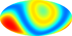
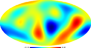
We then minimize $\Gamma$ over the range of parameters for both template types. It turns out that in neither case do we find one clear optimal solution: there are numerous templates that find $\Gamma\approx 0$ within the limitations of computational accuracy and the rotation grid. This is due to the small $\ell$-range but also due to the fact that the observed data is such a bad fit, with a very low $\chi^{2}$. Note that we are limited to this narrow $\ell$-range by our choice of models as this is where their power lies.

Given the degeneracy of our solution we have to impose an additional condition to select the preferred templates. Considering that the full (unsolvable) problem requires solving (11) we may break the degeneracy by evaluating the $\chi^{2}_{\ell}$ and defining

$$\Delta=\sum_{\ell}\left(\frac{\chi^{2}_{\ell}}{2\ell+1}-1\right)^{2}$$ (16)

By minimising $\Delta$ we find the solution of the abridged problem that’s closest to the solution to the full problem. Then the corrected map will have the power spectrum closest to the expected power spectrum line. This also breaks the degeneracy between the two $\alpha$ solutions associated with each template (see equation 7).

We find that our preferred Bianchi template has $x=1.4$ with left handed vorticity, and Euler angles $(\phi,\theta,\psi)=(-82,72,-62)$, and therefore an axis in the direction $(l,b)=(-62,18)$ in galactic coordinates. We find the preferred large Wave template has $\lambda=0.96$ and $\rho=44^{o}$, in the direction $(l,b)=(-38,30)$ (equivalently a wave in the opposite direction with $(l,b)=(142,-30)$ and phase $\pi-\rho$). That is, the preferred wave is just slightly smaller than the size of the CMB.

We examined the “Axis of Evil” behavior of the corrected maps (evil, ), and results are in Table 1 and Figure 1. We define a direction for each multipole by finding the $m$ and the direction ${\bf n}$ that maximises

$$r_{\ell}=\frac{C_{\ell m}(\bf n)}{(2\ell+1){\hat{C}}_{\ell}}$$ (17)

where $C_{\ell 0}=|a_{\ell 0}|^{2}$, $C_{\ell m}=2|a_{\ell m}|^{2}$ for $m>0$ (notice that 2 modes contribute for $m\neq 0$) and $(2\ell+1){\hat{C}}_{\ell}=\sum_{m}|a_{\ell m}|^{2}$. This finds the axis for which a multipole is most dominated by just one $m$-mode. As can be seen in Table 1, the uncorrected map finds similar directions for the $\ell=2,3,4,5$ multipoles (as reported in evil ) - a significant departure from isotropy. We see that the corrected maps find no such anisotropic behaviour. The average inter-$\ell$ angles found are perfectly consistent with isotropy as compared to simulations.

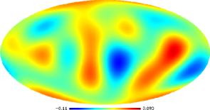
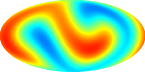
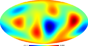
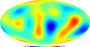
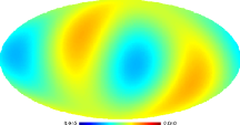
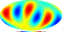
In Figures 2 and  3 we plot the map before and after the correction, only showing the multipoles $\ell=2-5$. In Figure 4 we plot the much examined Quadrupole and Octopole before and after the corrections. The alignment (biel, ; teg, ; copilet, ) can clearly be seen in the before maps, and not in the after maps, also the anomalously low power is increased, see Figure 5.

We have therefore proved that all known large-angle anomalies may be coupled. There are models providing templates which can correct, in one go, all known anomalies – the low power and the “axis of evil” effect. Whether or not the evidence for these models is high is another matter, which we now proceed to examine.

Figure 4: The Quadrupole, $\ell=2$ (above), and the Octopole , $\ell=3$ (below), for the uncorrected (left) and Bianchi corrected (middle) and the Wave corrected (right) maps. The apparent alignment is not present in the corrected maps (mK units).

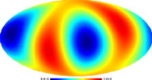
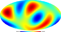
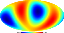
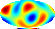
Bianchi

Wave

Figure 5: The power spectrum (mK²) of the map before (solid line) and after (long-dashes) being corrected for the preferred template (dotted). The $\Lambda$CDM theoretical power spectrum from WMAP is also plotted (short-dashes).

V Significance

There are many ways to quantify the significance of the final correction. As already noted in Section I, the expected power spectrum of a map will be higher than that for a purely Gaussian map if we assume the presence of a template. Thus, when considering the low-$\ell$ low power, if we take into account the presence of a template, then we actually make the situation worse! We consider simulations of Gaussian maps with the added template, for both the Bianchi and the Wave models. We calculate power spectrum estimator for 5000 simulations and indeed we find that the without adding a template, only 2.6% of simulations find a $C_{2}$ lower than that observed by WMAP. And with the Bianchi template added this reduces to 1.2%, thus making the fit worse.

However in apparent contradiction to this we have a map that, when corrected for the preferred template, finds excellent consistency with the theoretical power spectrum. So, we ask a different question here. We allow 1000 simulations to find their best template, for both model types. We record the $\chi^{2}_{d}$ before the correction, and the $\alpha$, $\chi^{2}_{t}$, $\Delta$ of the correction, and we only look at those simulations that find a low initial $\chi^{2}_{d}$ (525 of our 1000 simulations). We can now assess the significance of our results, given the prior assumption of a destructive alignment between the Gaussian process and the template.

We find the simulations return similar results to the WMAP map. That is we looked at the range of $\alpha$ values returned, and various functions of ($\alpha,\chi^{2}_{t},\Delta,\chi^{2}_{d}$) and found our WMAP result to not be particularly anomalous compared to the simulation results. This was the case for both the Bianchi and the Wave templates.

We therefore must conclude that the detections are not significant. However, we find the method still of interest, and note it can be used to investigate new models of contamination in the future. We give one example of a possible improvement.

Qualitatively the crux of the issue lies in that we must rely on a chance anti-alignment of phases between template and Gaussian process. We don’t see power in some $m$ modes because it was there both in the template and in the Gaussian process and the two added destructively. This will always sound suspicious and we suggest that models might be set up where the underlying non-Gaussian process influences the production of Gaussian fluctuations so that the two processes are anti-correlated. Specifically we could have set up a likelihood where the $\chi^{2}$ functions for template and Gaussian process added (rather than their $a_{\ell m}$). However such work is beyond the scope of this paper.

VI Discussion

We found templates from two different models that can simultaneously explain the observed anisotropic alignments of the low-$\ell$ multipoles and their low power. The corrected maps show power spectra vastly more consistent with the standard $\Lambda$CDM theoretical power spectrum (wmap, ) than the uncorrected map. The scope of our work was two-fold.

Firstly, we proposed a formalism for dealing with templates in the presence of data which has a low chisquared. In this approach we promote the $\chi^{2}$ to the status of relevant function of the data for comparing theory and data. This is in contrast with the the usual $a_{\ell m}$s, and reduces the number of degrees of freedom. Furthermore the likelihood problem is then turned on its head in that it enforces the strong prior that a Gaussian process with a power known a priori must be present in the corrected maps. Thus this approach generalizes the previous one in that it reduces to it for cases where the data chisquared is too high, but leads to significantly different results when the observed chisquared is too low.

Notice that standard methods for template correction will lead to a corrected map with a lower $\chi^{2}$. This is because it is more probable that the presence of a template will increase the power than remove it. We are therefore always on the back foot when trying to use a template to explain a low power spectrum (see slosar ; slosar2 for a similar discussion). We note that as the current data is such a bad fit, most of our templates ($\sim$90 %) improved the $C_{2}$ fit before we even imposed the second condition of minimising $\Delta$.

The second purpose of our paper was to use this formalism to investigate whether the low power (i.e. low chisquared) observed in the low multipoles and the axis of evil effect might be related to each other, and whether both could be due to an underlying anisotropic or inhomogeneous model of the Universe. The axis of evil effect consists of the fact that for a given $z$-axis orientation the power in a given multipole is not distributed “at random”among the various $m$ modes but concentrates on planar models ($m=\pm\ell$) for $\ell=2,3$; furthermore the axis for which this happens is roughly the same for $\ell=2,...,5$. A priori the two effects should be coupled because the $C_{\ell}$ is an average over $m$ of the variance $|a_{\ell m}|^{2}$. It looks as if some $m$-modes missed their power and that if this was reinstated the low $C_{\ell}$ and the “axis of evil” anomalies would disappear. This might happen after correcting the nefarious influence of a deterministic template and it suggests that the template should have a strong non-planar component along the preferred direction.

We considered Bianchi models and also inhomogeneous models where a very strong long-wavelength wave is part of the background model. We find the preferred parameters for these models and correct the maps. The corrected maps are free of anomalies, in particular their quadrupole and octupole are not planar and their intensities not low. Therefore we stress that although the “template” detection are not found to be statistically significant they do correct statistically significant anomalies.

While this paper was being finished two preprints appeared proposing explanations for the axis of evil effect pancake ; sib . One of these is rather similar in spirit to ours sib : the idea that a long wavelength mode is imprinted in the sky. Even though our statistical treatment is rather different, both papers highlight the same difficulty with such explanations: that in general waves would add, rather than subtract power. Our suggested explanation (that an anti-correlation might exist between the Gaussian and the deterministic process) finds its counterpart in the model considered in sib in the concept of multiplicative non-linear response. We find this idea very interesting, but as with our idea of Gaussian/template anti-correlation we stress that it may not be necessary. The fit between the data and the pure Gaussian model is so bad that a fluke anti-alignment of phases is already a good enough explanation (even though clearly the Bayesian evidence for more complex models will always be superior).

We are also examining the possible correlations between the CMB anomalies and the large-scale structure and defer to a future publication ofer comments on pancake .

Acknowledgements We thank Anthony Banday, Kris Gorski, Andrew Jaffe, Tesse Jaffe, João Medeiros, Carlo Contaldi, and Max Tegmark for helpful comments. Our calculations made use of the HEALPix package healp and were performed on COSMOS, the UK cosmology supercomputer facility. KL is funded by PPARC.

References

- (1) Banday A.J., Zaroubi S., Gorski K.M., astro-ph/9908070.
- (2) Barrow J., Juszkiewicz R., Sonoda D.H., 1985, MNRAS, 213, 917
- (3) Bennett C.L. et al., 2003, Astrophys. J. Suppl, 148, 1
- (4) Bennett C.L., et al., 2003, ApJS, 148, 97.
- (5) Berera A., Buniy R., Kephart T., hep-th/0311223.
- (6) Bielewicz P., Gorski K., Banday A.J., astro-ph/0405007.
- (7) Bridle S., et al., Mon.Not.Roy.Astron.Soc. 342: L72, 2003.
- (8) Bunn E.F., Ferreira P., Silk J., astro-ph/9605123.
- (9) Coles P., et al., 2003, astro-ph/0310252;
- (10) Coles P., astro-ph/0502088.
- (11) Contaldi C., et al, JCAP 0307: 002, 2003.
- (12) Copi C.J., Huterer D., Starkman G.D., Phys.Rev. D70, 043515, 2004.
- (13) Cornish N., et al, Phys. Rev. Lett. 92, 201302, 2004.
- (14) de Oliveira-Costa A., et al., 2004, Phys. Rev, D69, 063516
- (15) Efstathiou G., 2004, Mon.Not.Roy.Astron.Soc. 348:885,2004
- (16) Eriksen H.K., et al., 2004, Astrophys. J, 605, 14
- (17) Eriksen H.K., et al., 2004, astro-ph/0401276
- (18) Eriksen H.K., et al., 2004, astro-ph/0407271
- (19) Eriksen H.K., et al., ApJ, 612, 633, 2004 [astro-ph/0403098].
- (20) Ferreira P., Magueijo J., Górski K., 1998, Astrophys.J, 503, 1
- (21) Ferreira P., Magueijo J., Phys. Rev. D56: 4578-4591, 1997.
- (22) Gordon C., et al, astro-ph/0509301.
- (23) Górski K.M., Hivon E., Wandelt B. 1998, astro-ph/9812350
- (24) Hansen F.K., Banday A.J., Górski K.M.,2004,astro-ph/0404206
- (25) Hansen F.K., et al., 2004, astro-ph/0402396
- (26) Hinshaw G., et al., 2003, ApJS, 148, 63.
- (27) Hipolito-Ricaldi W.S., Gomero G.I., astro-ph/0507238.
- (28) Jaffe A., et al., astro-ph/0301077.
- (29) Jaffe T., et al., astro-ph/0503213.
- (30) Kogut A., Hinshaw G., Banday A.J., 1997, Phys. Rev. D, 55, 4, 1901
- (31) Kolb E.W., Matarrese S., Riotto A., astro-ph/0506534.
- (32) Krasinski A., Inhomogeneous Cosmological Models, Cambridge University Press, 1997.
- (33) Lahav O., Land K., Magueijo J., Rassat A., in preparation.
- (34) Land K., Magueijo J., 2004, MNRAS 357, 994, 2005.
- (35) Land K., Magueijo J., Phys.Rev.Lett. 95, 071301, 2005.
- (36) Land K., Magueijo J., MNRAS 362, L16, 2005.
- (37) Land K., Magueijo J., MNRAS 362, 838, 2005.
- (38) Land K., Magueijo J., astro-ph/0507289.
- (39) Magueijo J., 2000, Astrophys. J. Lett, 528, 57
- (40) Magueijo J., Medeiros J., 2004, MNRAS 351, L1-4
- (41) Magueijo J., 1995, Phys. Lett, B342, 32. Erratum-ibid, B352, 499.
- (42) Maxwell J., A treatise on Electricity and Magentism, Vol.1, Dover Publications, NY, 1954.
- (43) Moffat J., astro-ph/0502110.
- (44) Ralston J., Jain P., Int. J. Mod. Phys. D13, 1857, 2004.
- (45) Roukema B., et al., astro-ph/0402608.
- (46) Schwarz D., et al., Phys.Rev.Lett. 93: 221301, 2004.
- (47) Slosar A., Seljak U., . Rev. D70: 083002, 2004.
- (48) Slosar A., Seljak U., Makarov A., astro-ph/0403073.
- (49) Tegmark M., de Oliveira-Costa A., Hamilton A., Phys.Rev. D68: 123523, 2003.
- (50) Vale C., astro-ph/0509039.
- (51) Vielva P., et al., 2003, astro-ph/0310273
- (52) Weeks J., et al., Mon. Not. Roy. Astron. Soc. 352, 258, 2004.