Boundary Inflation and the WMAP Data
Abstract
Inflation in a five-dimensional brane world model with two boundary branes is studied. We make use of the moduli space approximation whereby the low energy theory reduces to a four-dimensional biscalar-tensor gravity plus a minimally coupled scalar field. After a detailed analysis of the inflationary solutions, we derive the evolution equations of the linear perturbations separating the adiabatic mode from two entropy modes. We then examine the primordial scalar and tensor power spectra and show that their tilt depends on the scalar-tensor coupling constant. Finally, the induced CMB anisotropies are computed and we present a Monte Carlo Markov Chains exploration of the parameter space using the first year WMAP data. We find a marginalized probability bound for the associated Eddington parameter at the end of inflation , at confidence level. This suggests that future CMB data could provide crucial information helping to distinguish scalar-tensor and standard inflationary scenarios.
pacs:
04.50.+h, 11.10.Kk, 98.80.CqI Introduction
Although the standard particle physics and cosmological models in a four-dimensional spacetime provide an accurate enough description of particle physics experiments and cosmological observations Eidelman et al. (2004), considering unseen extra dimensions allows one to make theoretical progress towards a Unified Theory of all interactions Nordström (1914); Kaluza (1921); Klein (1926); O’Raifeartaigh and Straumann (2000); Polchinski (1998a, b). The advent of M-theory and branes has led to the “brane world” concept in cosmology. Motivated by the Hořava–Witten model and its compactifications Horava and Witten (1996); Witten (1996), brane world models assume that we are living on a higher dimensional spacetime boundary (brane).
In cosmology, brane worlds have been studied within the framework of five-dimensional (5D) models and lead to only a few observable predictions (see Refs Langlois (2003); Maartens (2004); Brax et al. (2004) for a review and references therein). Models ranging from classical membrane theories of General Relativity to topological defect models have been studied in various compact or non-compact, curved or flat, symmetric or non-symmetric, extra dimensional spacetimes, as well as their associated deviations, or incompatibilities, with respect to the standard cosmology Akama (1982); Rubakov and Shaposhnikov (1983); Davis et al. (2001); Battye and Carter (1995); Battye et al. (2001); Binetruy et al. (2000); Maartens et al. (2000); Randall and Sundrum (1999a, b); Garriga and Tanaka (2000); Arkani-Hamed et al. (1998); Antoniadis et al. (1998); Ringeval et al. (2003); Dvali et al. (2000); Antoniadis et al. (2003); Cremades et al. (2002); Kokorelis (2004); Kohlprath (2004); Kolanovic et al. (2003); Ringeval and Rombouts (2005); Cvetic and Soleng (1997); Bonjour et al. (1999); Antunes et al. (2002); Ringeval et al. (2005); Koyama et al. (2004); Cartier and Durrer (2005). Definite cosmological predictions remain however difficult to extract in the high energy limit where the universe evolution is strongly affected by the physical processes occurring in the extra dimensions. On the other hand, at lower energy scales (typically smaller than the brane tension) it appears possible to describe such systems by effective four-dimensional actions.
In the framework of five-dimensional compactifications of M-theory Lukas et al. (2000, 1999), the moduli space approximation describes, through a four-dimensional effective action, a system of two branes of opposite tension embedded in a five-dimensional warped spacetime Brax and Davis (2001). Besides the fields living on the positive tension brane (assumed to be our universe), the moduli associated with the position of the branes in the fifth dimension act as two non-minimally coupled scalar fields thereby leading to an effective biscalar-tensor theory of gravity Ashcroft et al. (2004a); Brax et al. (2003a); Kobayashi and Koyama (2002); Brax et al. (2003b); Ashcroft et al. (2004b); Kanno and Soda (2004); Palma and Davis (2004a); Davis et al. (2005). Scalar-tensor theories have been intensively studied as natural extensions of General Relativity and are strongly constrained in the solar system Damour and Esposito-Farese (1992); Will (2001). On the cosmological side, there are (weaker) constraints coming from the Big Bang Nucleosynthesis (BBN) and recent works have been focused on scalar-tensor effects in the Cosmic Microwave Background anisotropies (CMB) and in weak gravitational lensing Damour and Pichon (1999); Perrotta et al. (2000); Chen and Kamionkowski (1999); Baccigalupi et al. (2000); Amendola (2001); Riazuelo and Uzan (2002); Nagata et al. (2004); Acquaviva et al. (2005); Esposito-Farese (2004); Uzan (2005); Schimd et al. (2005); Rhodes et al. (2003). In these works, scalar-tensor theories have been discussed in the context of the post-inflationary cosmology by quantifying the distortions the non-minimally scalar fields may induce compared to the pure General Relativity predictions. In fact, even if the cosmological constraints are currently weaker than the solar-system ones, they are complementary in the sense that they probe the cosmic times. This is relevant since it has been shown that scalar-tensor gravity models can relax towards General Relativity during the cosmological evolution Damour and Nordtvedt (1993). As a result, such models may have no observable impact in the post-inflationary eras, and in particular in the solar system, while modifying significantly the dynamics of the early universe.
On top of probing the post-inflationary eras, the precision reached by the current CMB experiments allows one to constrain the shape of the power spectra of the primordial cosmological perturbations. Recast in the inflationary context, this is an opportunity to shed light on the physics at earlier times and in particular the deviations scalar-tensor theories may generate during inflation.
In this paper, we are interested in the primordial inflationary eras occurring in a boundary inflation model and their potential observable effects in the CMB, given the first year Wilkinson Microwave Anisotropies Probe (WMAP) data Kogut et al. (2003); Verde et al. (2003); Hinshaw et al. (2003). A minimal realistic three-fields model is considered: two of them being the moduli associated with the position of the branes in the extra dimension, and the other acts as a standard inflaton field living on our brane and coupled to the matter sector Brax et al. (2003a); Kobayashi and Koyama (2002); Brax et al. (2003b); Ashcroft et al. (2004b); Palma and Davis (2004b). After a detailed analysis of the several viable background evolutions, we compute and discuss the primordial power spectra of the scalar and tensor perturbations generated during inflation. We then derive the resulting CMB anisotropies and perform a Monte Carlo Markov Chain exploration of the parameter space in a regime where the deviations from General Relativity predictions are dominated by the shape of the primordial power spectra. By comparing the power spectra induced by the standard chaotic inflaton field alone and the ones obtained by considering the moduli, we find that the first year WMAP data can differentiate between standard chaotic and boundary inflation. In fact, for a given matter sector, the presence of non-minimally coupled scalar-fields during inflation changes the tilt of the primordial power spectra due to the running of the conformal factor. In our framework, we find the presence of the moduli statistically disfavored by the data, either as the WMAP data are insensitive to their effects when they are weakly coupled, or as they lead to a strongly tilted power spectra. These effects lead to an upper bound on the allowed values of the moduli coupling constant during inflation, which can be recast in terms of the more commonly used Eddington post-Newtonian parameter Will (2001): . On one hand, this bound holds at the time of inflation and, according to the above discussion, provides a very early constraint on scalar-tensor theories. On the other hand, it relies on the running of the conformal factor during inflation as well as the choice of the matter sector. In particular, one may expect this bound to be modified, or evaded, with more complicated potentials for the matter fields, or by freezing the running of the conformal factor at the time where observable cosmological perturbations were generated. Nevertheless, this result suggests that the current and future CMB data can be used to probe scalar-tensor theories as early as during the inflationary era.
In Sect. II, the boundary inflation model is introduced and the background inflationary evolutions solved both analytically and numerically. Sect. III is devoted to the derivation of the linear perturbations around the background evolution by means of a separation between the adiabatic and the two entropy modes. The equations of motion obtained are solved numerically and used to compute the resulting primordial power spectra at the end of inflation. In Sect. IV, we use modified versions of the public CMB codes camb Lewis et al. (2000) and cosmomc Lewis and Bridle (2002), linked with our inflationary code, to probe the boundary model parameter space given the WMAP data. Finally, the relevance and the possible improvements of our results are discussed in the conclusion, and the possibility of using the CMB to accurately probe scalar-tensor theories in the early universe is raised.
II Background evolution
We will focus on the low energy effective theory of 5D brane world models with a bulk scalar field and matter living on the positive tension brane. In this context, the low energy degrees of freedom of the model are the graviton leading to 4D gravity, the bulk scalar field zero mode and the inter brane distance, i.e. the radion. One can also parametrise the two scalar modes as the two brane positions. In the following we will denote by and the two moduli which are related to the brane positions and by
| (1) | ||||
where fixes the energy scale of the brane tensions and is a constant which determines how warped the extra dimension is Brax and Davis (2001); Brax et al. (2003a); Ashcroft et al. (2004b). In particular for , we obtain the Randall–Sundrum case. The four-dimensional (4D) gravitational coupling is related to the 5D gravitational coupling via
| (2) |
Using these relations one gets
| (3) | ||||
and
| (4) |
Notice that and when the two branes collide. On the contrary, and correspond to the negative tension brane being stuck at the bulk singularity and the positive tension brane receding away towards infinity. This situation will happen during the inflationary evolution.
Denoting by the minimally coupled scalar field living on our brane universe, the effective action in the Einstein frame, with a metric of signature, reads
| (5) | ||||
where and stands for the moduli fields, is the conformal factor, the moduli bulk potential and the minimally coupled scalar field potential on the brane. In the following, we will focus on the minimal setup of Refs. Brax et al. (2003a), i.e.
| (6) | ||||
In terms of the 5D picture, parametrises the coupling of the bulk scalar to the brane. Since the resulting four-dimensional theory is of multiscalar-tensor kind, it is also convenient to introduce the first conformal gradient
| (7) |
These are the gravitational couplings of the two moduli. Their present values are constrained by solar system experiments. Moreover, we will assume a chaotic-like potential for
| (8) |
In such a setup, the field is expected to be coupled to the observed form of matter and it will be referred to as the “matter field” in the following. As in the standard chaotic model, inflation can be driven by , but also by the moduli as discussed in the next section Kofman et al. (2004).
II.1 Basic equations
II.1.1 Sigma-model formalism
For the sake of clarity it is more convenient to recast the action (5) in terms of a non-linear sigma-model Damour and Esposito-Farese (1992); Damour and Nordtvedt (1993); Koshelev (2004)
| (9) |
the field-manifold being defined through
| (10) |
where the dimensionless scalar field has been introduced. From Eq. (6), the fields evolve in the potential
| (11) |
In the following, it will be implicitly assumed that the Latin indices refer to the field-manifold. Differentiating the action (9) with respect to the metric leads to the Einstein-Jordan equations
| (12) |
with the source terms
| (13) |
where
| (14) |
Similarly, the fields obey the Klein-Gordon-like equation
| (15) |
where denotes the Christoffel symbol on the field-manifold
| (16) |
and should be understood as the vector-like partial derivative of the potential
| (17) |
II.1.2 Equations of motion
In a flat Friedman–Lemaître–Robertson–Walker (FLRW) Universe with metric
| (18) |
being the conformal time, the equations of motion (12) and (15) simplify to
| (19) | ||||
| (20) | ||||
| (21) |
where a prime denotes differentiation with respect to the conformal time and is the conformal Hubble parameter . In the Einstein Frame, the “new terms” compared to minimally coupled scalar multifield inflationary models are encoded in the sigma-model metric and the Christoffel symbols .
Since we are interested in inflationary behaviour, it is more convenient to work in terms of an “efold” time variable
| (22) |
Apart from being the relevant physical time quantity during an inflationary era, when expressed in terms of , the field equations can be decoupled from the metric evolution Collins (1971, 1972); Shikin (1973); Damour and Esposito-Farese (1992); Damour and Nordtvedt (1993) and Eqs. (19) to (21) separate into
| (23) | ||||
| (24) | ||||
| (25) |
The dot denotes differentiation with respect to , the physical Hubble parameter is , and the field velocity (in efold time) on the manifold is
| (26) |
This is the derivative of the so-called adiabatic field. Indeed, differentiating Eq. (24) and using Eq. (25) yields the standard second order differential equation for the adiabatic field , i.e. in conformal time Gordon et al. (2001); Di Marco et al. (2003)
| (27) |
where are unit field-vectors along the classical trajectory
| (28) |
As mentioned above, the fields evolution is decoupled from the Hubble flow and Eq. (25) mimics the evolution of a “particle” of variable inertia on a curved manifold in presence of friction and an external force Damour and Esposito-Farese (1992); Damour and Nordtvedt (1993). From Eqs. (6) and (8) one gets
| (29) | ||||
while the only non-vanishing sigma-model Christoffel symbols are
| (30) | ||||
where lowering and raising indices on the first conformal gradients is performed with the field-manifold metric . The fact that the effective potential for the fields is ensures that the evolution of the fields in efold time is independent of any multiplicative constant appearing in the definition of the matter potential , as in the chaotic-like potential we are interested in [see Eq. (8)]. Obviously, still fixes the normalisation of the Hubble parameter in Eq. (23) and is directly related to the amplitude of the power spectrum of linear perturbations.
From Eqs. (25) and (29), we can draw the qualitative evolution of the fields. Starting from reasonable initial conditions, i.e. [see Eq. (23)], the friction terms will tend to produce a stationary regime in which the fields relax toward the minimum of the potential . For instance, the dilaton field will relax toward vanishing value as fast as
| (31) |
and stays frozen at afterward, whereas grows as
| (32) |
From Eq. (29), the matter field is expected to slowly evolve from its initial value provided , thereby allowing a period of slow-roll inflation Ashcroft et al. (2004a). However, since the force term involves also the conformal factor , the properties of the inflationary era, as its duration and end, will be certainly dependent on the evolution of the moduli fields and .
In the next section, we will present some analytical approximations and numerical solutions to the previous sketch.
II.2 Inflationary solutions
II.2.1 Scale factors acceleration
Since we are dealing with a multiscalar-tensor theory, it is convenient to clarify the definition of “inflation” in the cosmological context. The frame where non-gravity measurements take their usual form is the Jordan frame where matter is minimally coupled to the metric. For a given conformal coordinate system, the metric tensor in the Jordan frame is obtain from the metric tensor in the Einstein frame by the conformal transformation
| (33) |
As a result, the acceleration of the scale factor is not necessarily the same in the Jordan and Einstein frame and may even take place in one frame only Esposito-Farese and Polarski (2001). To solve the flatness and homogeneity problem, we are interested in inflationary era in the Jordan frame, i.e. when the first slow-roll parameter in that frame
| (34) |
From Eq. (33), the conformal Hubble parameter in the Jordan frame is also
| (35) |
where the dot denotes again the derivative with respect to , the total number of efold in the Einstein frame. From Eq. (34), one gets
| (36) |
where is the first slow-roll parameter in the Einstein frame and is the second conformal gradient defined as
| (37) |
In our setup, from Eqs. (6) and (7), its only non-vanishing value is
| (38) |
which rapidly vanishes for non-vanishing values of . Moreover, in a friction dominated regime , the remaining term in Eq. (36) can be significant only at the time when both and are non-vanishing, i.e. when the field leaves the friction dominated regime, where it was decreasing with constant velocity, to be frozen on the attractor at . As the result, we can expect as long as the fields remain in the friction dominated regimes.
II.2.2 Minimal slow-roll approximations
From the Einstein equation (24), the first slow-roll parameter in the Einstein frame is simply related to the field velocity by
| (39) |
Putting everything together in Eq. (25) yields
| (40) | ||||
| (41) | ||||
| (42) |
The friction dominated evolution of the moduli fields discussed in the previous section is recovered provided we assume the matter field to be in slow-roll . In this limit, Eqs. (41) and (42) admit the solutions
| (43) |
where it was assumed that . However, note that is an exact solution of Eq. (42) and thus, may be non-vanishing only during less than a few efolds of transition between and . Let us point out that the derivation of Eq. (43) does not require all the fields to be in slow-roll, and in particular may not be small Linde (2001). This is due to the simple form of the conformal factor we are interested in, whereas in the generic case a full slow-roll treatment may be required Noh and Hwang (2001); Di Marco and Finelli (2005). In the two regimes and , the conformal factor evolves as
| (44) |
with for , and for . In both cases, since we are assuming , we have [see Eq. (39)]. The moduli are thus driving two expansion eras with
| (45) |
In our setup, according to Eq. (6), the first era is not inflation since , whereas the second one is for values of the coupling constant . Physically, it means that starting from high values of only gives rise to a period of non-inflationary expansion where the moduli relaxes toward , and consequently, the effective Planck length decreases exponentially. When reaches its attractor, an inflationary era driven by can start, which also corresponds to a decreasing effective Planck length [see Eq. (44)].
In terms of the 5D picture, the fate of the moduli indicates that the two branes move away from each other. The inflationary phase driven by occurs once the right (negative tension) brane becomes close enough to the bulk singularity. As is constant in this regime, the energy density of the boundary inflaton is constant leading to a constant detuning of the left brane tension. As already studied in Brax and Davis (2001), this leads to an accelerated phase with an exponential potential and power law inflation. More details about this power law inflation phase can be found in Ref. Brax et al. (2003b).
This picture remains valid provided and from Eqs. (40) and (43) we can check the consistency of this approximation. From Eq. (44), if starts from large enough values such that then an approximate solution of Eq. (40) is
| (46) |
In this case, we have indeed
| (47) |
and the matter field remains frozen at its initial value until , i.e. during approximately
| (48) |
efolds after which Eq. (46) is no longer valid. Then the field starts to evolve and increases until for which inflation ends. Nevertheless, the standard slow-roll approximation can be used to derive the behavior of the matter field during this last phase. For reasonable small value of , ends up being dominated by the matter field evolution [see Eq. (39)] whereas the behavior of the moduli remains almost the same. Indeed, as can be seen in Eq. (41), the value of will be affected up to only by the matter field when , which is also the end of inflation [see Eq. (39)]. As a result, Eq. (44) is still a good approximation for the conformal factor, and using the slow-roll approximation in Eq. (40) leads to
| (49) |
where the “sr” indices label the efold at which . The end of inflation occurs for which gives the number of efolds in this last stage
| (50) |
Note that in the limit , we recover the usual one-field slow-roll expression for a chaotic potential Martin (2004)
| (51) |
with .
II.2.3 Numerical approach
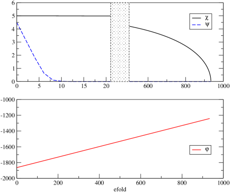
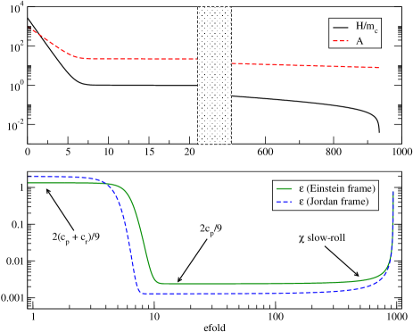
A numerical integration of the equations of motion (23) to (25) has been performed and illustrates the analytical behavior described in the previous section. In Fig. 1, the three expansion eras can be distinguished by means of the values. For the chosen model parameters, during the first ten efolds, the field relaxes towards zero and its evolution dominates the expansion. As previously pointed out, this is not an inflationary era in our model. During this phase, the conformal factor, and thus the Hubble parameter, decrease exponentially [see Eqs. (11) and (23)].
Once reaches its minimum, the dynamics are dominated by the second moduli and . Note that during the transition between these two regimes, the slow-roll parameter and , in the Einstein and Jordan frames respectively, do not match, as expected from Eq. (36). As can be seen on Fig. 1, inflation (in the Jordan frame) starts a few efolds before in the Einstein frame. During the dominated inflationary era, the matter field leaves its initial value and starts to slow-roll under the external force [see Eq. (29)] leading to the observed variation of after . The last stage occurs when the inflation is mainly driven by and we recover a one-field like behavior until for which inflation stops. Note that, as expected from the analytical study, even in this last regime, the evolution of the moduli and is not significantly affected by the rolling of the matter field. As a result, their second derivatives remain small and at the end of inflation (see Fig. 1).
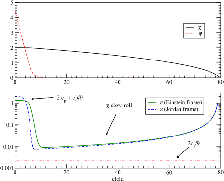
The above settings can nevertheless be affected according to the parameter values and the initial conditions. Indeed, the matter field can leave its initial value as soon as, or even before, the end of the domination expansion. In that case, as can be seen in Fig. 2, there is no time for a pure dominated inflation and after a intermediate mixed phase, we jump directly to the last dominated stage.
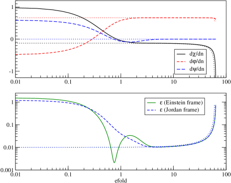
Concerning the initial conditions, it is important to mention that we have fixed the initial derivatives of the fields in such a way that their evolution start in the friction dominated regime, i.e. with an initial boost . In Fig. 3, we have plotted the behavior of the fields obtained for an arbitrary choice of reasonable initial velocities, i.e. verifying . As expected, it takes less than few efolds for the fields to relax toward their attractor behavior. As previously discussed, during the relaxation time, the slow-roll parameters in Einstein and Jordan frame are significantly different.
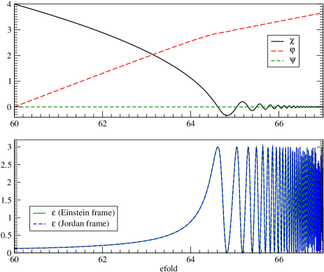
In order to derive the primordial perturbations produced in this model and the resulting cosmic microwave background anisotropies (CMB), it is necessary to assume a cosmological scenario for the background. Motivated by the brane world picture where the moduli and are related to the position of the branes in the five-dimensional spacetime, it is reasonable to consider that these two fields do not decay and remain present in the late-time cosmology. As a result, only can decay into radiation and dark matter at the end of inflation. In Fig. 4, we have plotted the fields evolution during a few efolds after the end of inflation, the matter field ends up oscillating thereby starting a period of reheating from which the radiation dominated era can begin Turner (1983); Shtanov et al. (1995); Kofman et al. (1997). Note that even if inflation can be driven by (see Sect. II.2), the presence of is still required to end it. The observational consequences coming from these assumptions will be more detailed in Sect. IV.
In the next section, the linear perturbations arising during the inflationary eras are discussed, as well as their primordial power spectra.
III Linear perturbations
III.1 Gravitational and matter sector
In the longitudinal gauge, the scalar perturbations (with respect to the rotations of the three-dimensional space) of the FLRW metric can be expressed as
| (52) |
where the indices and refer to the spatial coordinates only, and and are the Bardeen potentials. In the sigma-model formalism, denoting by the scalar perturbations of the fields, the Einstein-Jordan equations perturbed at first order are
| (53) | ||||
| (54) | ||||
| (55) |
where the prime stands for the derivative with respect to the conformal time and use has been made of (perturbed Einstein equation for ). The Laplacian reduces to
| (56) |
for flat spatial hypersurfaces. The perturbed equations of motion for the fields stem from Eq. (15) and read
| (57) |
The fact that there is more than one scalar field involved leads to the existence of entropy modes that can source the adiabatic mode. In the next section, we use the formalism developed in Refs. Gordon et al. (2001); Groot Nibbelink and van Tent (2002); Hwang and Noh (2002); Di Marco et al. (2003) to derive the evolution equations of the adiabatic and the two entropy modes arising in our model.
III.2 Adiabatic and entropy perturbations
III.2.1 Generic decomposition
From Eqs. (III.1) to (III.1), up to the background equations, the evolution of the Bardeen potential simplifies to
| (58) |
In terms of the comoving curvature perturbation Lukash (1980); Lyth (1985); Kodama and Sasaki (1984); Mukhanov et al. (1992); Durrer (1994); Martin and Schwarz (1998)
| (59) |
Eq. (54) yields
| (60) |
where the adiabatic perturbation is the perturbed version of Eq. (26) as well as the resulting perturbation of all fields projected onto the classical trajectory [see Eq. (28)]:
| (61) |
The dynamical equation (58) also reads
| (62) |
which can be recast into
| (63) |
The orthogonal projector is defined by
| (64) |
where is the first fundamental form of the one-dimensional manifold defined by the classical trajectory Carter (1997). We recover that the comoving curvature perturbation on super-Hubble scales () is only sourced by the entropy perturbations defined as the projections of all field perturbations on the field-manifold subspace orthogonal to the classical trajectory Martin and Schwarz (1998).
III.2.2 Spherical basis
For the studied boundary inflation model, the sigma-model manifold is three-dimensional which implies the existence of two entropy modes living in the two-dimensional subspace orthogonal to the classical trajectory. The decomposition performed in Refs. Gordon et al. (2001); Di Marco et al. (2003) is straightforwardly generalized by choosing a local spherical basis at each point of the fields trajectory. This can be performed by introducing the angular fields and defined by
| (65) |
and
| (66) |
provided and do not vanish at same times. They define an instantaneous rotation matrix on the field-manifold
| (67) |
which transforms the original fields into the adiabatic and entropy modes
| (68) |
The evolution of the angular fields is readily obtained by differentiating Eqs. (65) and (66) and using the background equations (19) to (21)
| (69) |
| (70) |
for and , respectively. The rotated potential derivatives have been defined through
| (71) |
Note that since we are dealing with non-minimally coupled scalar fields, they are not the partial derivatives of the potential with respect to the rotated fields Di Marco et al. (2003), however remains the effective potential which sources the adiabatic field [see Eq. (27)]. In the spherical basis, we recover explicitly that the entropy modes only source the comoving curvature perturbation since in Eq. (63) one has . In order to compute the primordial power spectra and the cross-correlation for the different modes, it is convenient to recast the equations of motion for the original fields in terms of the rotated modes only Langlois (1999); Gordon et al. (2001); Di Marco et al. (2003).
III.2.3 Equations of motion
The closed system of dynamical equations for the entropy and adiabatic modes can be obtained by expressing the second order derivative of each mode with respect to the conformal time in terms of the others by means of Eqs. (68) and (71), using Eqs. (19) to (21) as well as Eqs. (69) and (70) and their derivatives. Moreover, the adiabatic field can be expressed in terms of the comoving curvature perturbations by means of Eq. (60), which is a preferred observable for deriving the subsequent Cosmic Microwave Background (CMB) anisotropies (see Sect. IV). After straightforward but tremendous calculations one gets for the first entropy mode
| (72) | ||||
where use has been made of
| (73) |
and, from Eq. (63),
| (74) |
We have also introduced a rotated 2-form quantity (with respect to the field-manifold) from the potential according to
| (75) |
ensuring the symmetry properties
| (76) |
Note that the special form of the effective potential in Eq. (11) has been used to perform some simplifications
| (77) |
and
| (78) |
In Eq. (72), it was also convenient to introduce the exact potential derivative
| (79) |
Similarly, for the other entropy mode one gets
| (80) | ||||
The equation of motion Eq. (63) for can also be expressed in terms of the entropy modes only by differentiation
| (81) | ||||
In order to set quantum initial conditions during the inflationary eras, it is more convenient to use the Mukhanov variable Mukhanov et al. (1992) whose evolution is readily obtained from Eq. (81)
| (82) | ||||
The equations (72), (80) and (82) form a closed system of equations. Indeed the source terms involving the comoving curvature perturbation in Eqs. (72) and (80) can be expressed in terms of as
| (83) |
One can check that Eqs. (72), (81) and (82) match with the ones obtained for two fields in Refs. Di Marco et al. (2003); Ashcroft et al. (2004b) for , whereas Eq. (80) decouples and admits as a solution, up to transformation . As shown in Sect. II, since the dilaton relaxes toward rapidly, we expect to recover a two field like behavior also at the perturbation level. In the next sections we numerically solve the system of equations (72), (80) and (82) to compute the resulting power spectra at the end of inflation.
III.2.4 Numerical results
For a given background evolution (see Sect. II), and in the Fourier space with respect to the comoving spatial coordinates, the solutions of Eqs. (72), (81) and (82) are uniquely determined by the initial values of , , and their first order time derivative. Motivated by the quantum origin picture of the cosmological perturbations, in the Einstein Frame the scalar and tensor modes are decoupled and we can treat , and as independent stochastic variables deep inside the Hubble radius Mukhanov et al. (1992); Salopek et al. (1989); Tsujikawa et al. (2003); Martin (2004). Following the method of Ref. Tsujikawa et al. (2003), since we are interested in the two-point correlation function between the different rotated fields , and (or ), we will consider only the solutions obtained by starting with one mode in the Bunch-Davies vacuum while the others vanish, and the other mode permutations. In addition to providing enough information to compute all the power spectra, they clearly exhibit the sourcing effects of one field from the others. For numerical convenience, each Fourier mode will be assumed to appear at a given time such that
| (84) |
where is the comoving wave number and a constant verifying and characterizing the decoupling limit Salopek et al. (1989); Ashcroft et al. (2004b). For a Bunch-Davies vacuum, the value of does not usually change the power spectra, provided it is big enough to allow free wave solution111This is no longer true for trans-Planckian initial conditions Martin and Ringeval (2004); Easther et al. (2005).. For (and respectively , ), we therefore set at Kaloper et al. (2002); Martin and Brandenberger (2003)
| (85) |
In Fig. 5 the numerical solutions of Eqs. (72) to (82) have been plotted for the same background evolution as in Fig. 2 and for three different values of the comoving wave number with . In the top frame, the evolution of the Hubble parameter and the three physical wavenumbers are plotted as a function of the number of efold before the end of inflation (“bfold” in the following). A subtlety occurs however for the “very large” wavelength modes due to the existence of a non-inflationary era when the background evolution is dominated by the rolling of the field (see Sect. II and Fig. 2). Indeed, if the initial conditions in the five-dimensional setup are such that the initial value of is far from vanishing, then there are some perturbation modes which initially are super-Hubble and for which setting quantum initial conditions does not make sense. However, since we are interested in enough efolding to solve the flatness and homogeneity problems, such large wavelength modes are generically still super-Hubble today and thus non-observable. On the other hand, one cannot exclude that for a small number of efold, let’s say for instance, some of the large wavelength perturbation modes entering the Hubble radius today may have been created during the transition period between the dominated phase and the inflationary one, as in Fig. 5. Such a mode starts initially under the Hubble radius, but there is a maximum value of for which Eq. (84) has not solution (because would be too small). Our prescription is to discard the models for which observable perturbation modes today would have been created on Hubble, super-Hubble and sub-Hubble scales with initially.
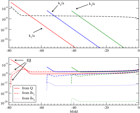
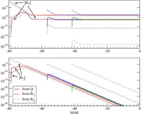
From the second to the bottom frame in Fig. 5, the evolution of , and are plotted, respectively. The straight, dashed and dot lines correspond to the three independent initial conditions for the modes, in a Bunch-Davies vacuum and , in a Bunch-Davies vacuum and , …, respectively. Moreover, in each frame we have plotted the three wavelength modes , and from the left to the right. In Fig. 6, we have plotted the real and imaginary parts of the comoving curvature perturbation for the mode associated with the solution of Fig. 5 and the background evolution of Fig. 2.
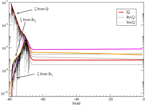
This plot shows the transition between the oscillatory behavior when the mode is under the Hubble radius and its damping on super-Hubble scales. However, since we are precisely in a multifields case, even on super-Hubble scales the comoving curvature perturbation slightly evolves sourced by the entropy modes till the end of inflation. Also, the rapid change in behavior of the Hubble parameter during the transition between the dominated era and the subsequent inflationary eras induces also a change of slope in the evolution of all the perturbation modes (see Fig. 5 and Fig. 6 around ). This can be understood by first noting that before the transition, as long as , the physical wavelength of the mode goes deeper into the Hubble radius with time whereas as soon as the wavelength becomes closer and leaves the Hubble radius. Moreover the amplitude of the sourcing effect of the entropy modes on the comoving curvature perturbation is enhanced. As can be seen in Fig. 5 and Fig. 6, the adiabatic mode is mainly produced by the entropy modes for whereas this effect progressively disappears for the bigger wavenumbers and . This comes from the fact that only the mode evolves and leaves the Hubble radius in a regime where the field is not yet vanishing (see Fig. 2). Note that in Eqs. (72) to (80), the Hubble parameter appears also in the effective potential of the modes. Its rapid (exponential) evolution during the relaxation of enhances the coupling between the entropy and adiabatic modes. Also, at the transition, the background fields are no longer in a stationary regime as discussed in Sect. II, and especially one expects and to increase and reinforces the coupling between the adiabatic and entropy modes. This effect is similar to the one observed for double-inflation models Tsujikawa et al. (2003). For the modes which evolve out of this stage, the field and its perturbations are negligible, i.e. and the second entropy mode decouples and decreases exponentially [see Eqs. (68), (80) and the bottom frame in Fig. 5]. The dynamics is close to a two fields like regime where the friction dominated evolution leads to a weakly coupled entropy mode Tsujikawa et al. (2003); Ashcroft et al. (2004b). As can been seen in Fig. 5, after Hubble exit, for the wavenumbers and , the entropy perturbations are quasi-frozen as it would be for a light scalar field.
III.3 Tensor modes
In the Einstein frame, the scalar and tensor degrees of freedom are decoupled. Therefore the equation of evolution for the tensor modes remains the same as in General Relativity. For a flat perturbed FLRW metric
| (86) |
where is a traceless and divergenceless tensor
| (87) |
one gets Mukhanov et al. (1992); Liddle and Lyth (1993)
| (88) |
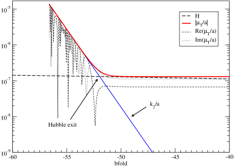
This equation can be numerically solved for each polarization state by setting the initial quantum tensor modes in the Bunch-Davies vacuum [see Eq. (85)]. In Fig. 7 their evolution has been plotted for wavenumber together with the evolution of the Hubble parameter. As expected for a massless field, the gravitational waves freeze on super-Hubble scales with where is the Hubble parameter at Hubble exit. Note however that the freezing occurs a few efolds after Hubble exit.
III.4 Primordial scalar and tensor power spectra
From the scalar and tensor modes evolution obtained in the previous sections, the primordial power spectra are readily obtained from the values taken by the adiabatic and entropy perturbations at the end of inflation. In the Fourier space and Einstein frame, the scalar power spectra are computed according to the method used in Ref. Tsujikawa et al. (2003), i.e.
| (89) |
where the observable perturbation modes stands for , and , whereas the index “” refers to the three independent quantum initial conditions. The tensor power spectrum reads
| (90) |
where the polarization degrees of freedom have been included.
In Fig. 8, we have plotted the typical power spectra associated with the solutions computed in Sect. III.2.4. The adiabatic power spectra is dominant compared to the two entropy ones and . Furthermore, the second entropy power spectrum is strongly damped and blue tilted compared to . In fact, this behavior is expected since the second entropy mode follows the evolution during inflation and vanishes exponentially with the total number of efolds. As a result, the earlier the modes cross the Hubble radius, the longer they sustain an exponential decay. Their power spectrum at the end of inflation is blue tilted since the smaller scales are accordingly less damped. However, since the observable perturbation modes are expected to cross the Hubble radius around efolds before the end of inflation, the entropy power spectrum cannot be significant at the end of inflation. In particular, the expected cross-correlations for -like modes discussed in Sect. III.2.4 are also washed out by such a damping. They can still be seen in Fig. 8 as a bump in the cross-correlation power spectra and , but with an extremely small amplitude. It is important to recall that the domination of during inflation has to occur before the last efolds of inflation since it drives a non-accelerated expansion in our model. As seen in Sect. II, this comes from the fact that whereas in a more generic scalar-tensor model with the transition from -dominated to -dominated inflation could be in the observable range and may generate a significant power spectrum for the second entropy mode Adams et al. (1997); Kaloper and Kaplinghat (2003); Hunt and Sarkar (2004). Nevertheless, we will accordingly be focused in the following on the present boundary inflation model where only the adiabatic, tensor and first entropy modes are of interest for the CMB Ashcroft et al. (2004b).
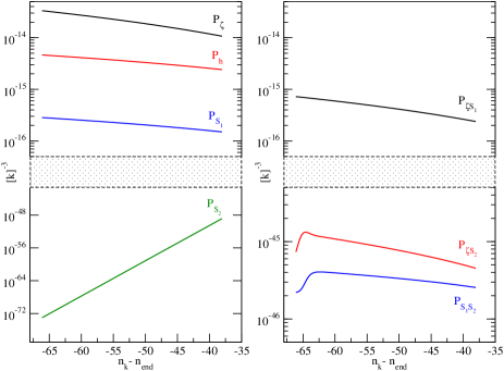
The hierarchy in the power spectra amplitudes can be qualitatively understood by noting that the entropy mode behaves almost like a free massless field for moderate values of the coupling constant . Indeed, as can be seen in Fig. 5, is weakly coupled to the adiabatic mode and remains almost frozen once it becomes super-Hubble. Neglecting the sourcing effects from the adiabatic modes, as well as the variation of the Hubble parameter during the few efolds after Hubble exit, one gets at the end of inflation
| (91) |
where is the dimensionless Hubble parameter at Hubble exit for each mode of wavenumber . From Eqs. (39) and (89), keeping in mind that at the end of inflation, the resulting power spectrum varies as
| (92) |
Similarly, assuming that the adiabatic mode gets massless field-like fluctuations at Hubble exit, in the weakly coupled regime the comoving curvature perturbation remains constant afterwards and the adiabatic power spectrum can be approximated by
| (93) |
where is the first slow-roll parameter at Hubble exit.
One can check in Fig. 8 that Eqs. (92) and (93) provide a good approximation of the relative power spectra amplitudes. Moreover, these equations show that the generated power spectra do not depend significantly on the initial values of the background fields which drive inflation. Indeed, as thoroughly discussed in Sect. II, the fields are rapidly attracted toward a friction dominated regime during which their evolution does no longer depend on their initial value. Obviously, the initial conditions determine the total number of efolds, but at a given efold before the end of inflation one may not expect to be strongly influenced [see Eq. (39)]. However, the amplitude of the perturbations at Hubble exit directly depends on the Hubble parameter value which involves both the bare mass of the matter field and the conformal factor . In order to disentangle their respective effects, it is more convenient to consider the effective mass of the matter field at the end of inflation
| (94) |
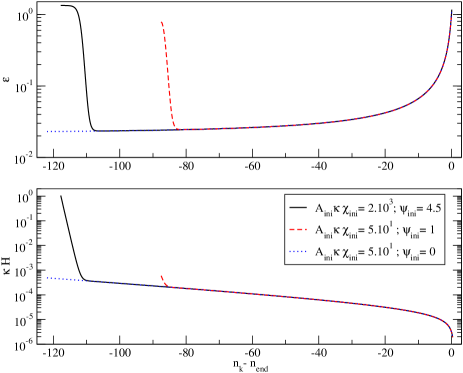
In Fig. 9, the slow-roll and Hubble parameters have been plotted for several arbitrarily chosen value of and , the other parameters and being fixed. As the plots show, the last efolds of evolution cannot be differentiated and we have checked by a direct computation that this is also the case for the corresponding power spectra at the end of inflation. In fact, the only effects and might induce concern the transition at the end of the -dominated expansion, which is, as explained before, hardly observable for the CMB.
The remaining degrees of freedom in the power spectra are the effective mass and the moduli coupling constant . These parameters are expected to have significant observable effects. On one hand, the effective mass fixes the overall amplitude of the Hubble parameter and is therefore directly related to the amplitude of the primordial perturbations. On the other hand, the coupling constant encodes how much the conformal factor may run during the generation of the observable perturbations. From Eq. (11), such a running renders the potential steeper and one may expect bigger tilts for the power spectra.
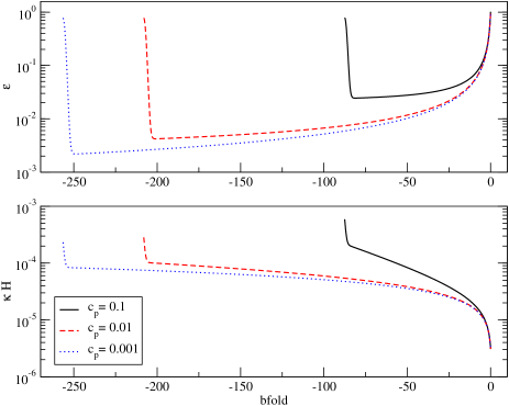
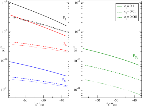
In Fig. 10, the slow-roll and Hubble parameters have been plotted for several values of , the effective mass at the end of inflation being fixed. The slopes of these two functions are effectively steeper for larger values of the coupling constant and the resulting power spectra may be qualitatively guessed from (92) and (93). The direct computations of the power spectra at the end of inflation have been plotted in Fig. 11 and confirm this behavior.
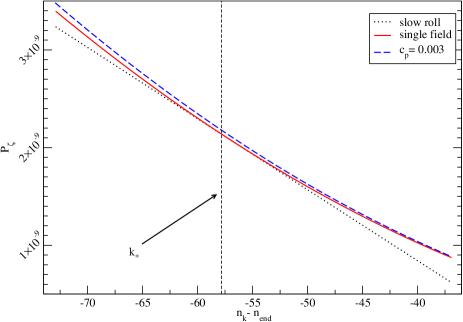
In order to dress a qualitative understanding of the above-mentioned effects, we have compared in Fig. 12 the adiabatic power spectrum generated during a weakly coupled boundary inflation with with the one associated with the standard single field chaotic inflation (). Moreover, we have plotted the first order slow-roll approximation of the chaotic model around a pivot scale . In this limit, the adiabatic power spectrum simplifies to Martin and Schwarz (2000)
| (95) |
where all the parameters are evaluated at the pivot scale. The constant and is the second slow-roll parameter. The deviations observed in Fig. 12 between the slow-roll and single field power spectra come from the natural running of the spectral index which is not grabbed by the first order slow-roll approximation. The differences between the chaotic and boundary spectra are due to the slight running of the conformal factor obtained for . More qualitatively, for non-vanishing values of the moduli coupling constant, the effective mass of the matter field is not constant during the generation of the observable perturbations and induces deviations with respect to a single field model.
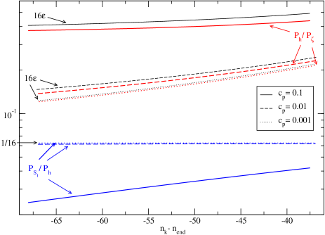
As previously pointed, Eqs. (92) and (93) are relevant only if the modes do not evolve significantly after Hubble exit. This is obviously the case for the single field model, but certainly no longer true for high values of the moduli coupling constant. In Fig. 13, we have plotted the ratio between the computed power spectra for several values of . Some deviations show up for in the ratio tensor to scalar and in the entropy modes Starobinsky and Yokoyama (1994); Garcia-Bellido and Wands (1995).
In the next section, after setting up a toy cosmological model, we use the above numerical method to derive the resulting CMB anisotropies and perform a Monte Carlo Markov Chains exploration of the model parameter space given the first year WMAP data. As expected from the behaviour of the primordial power spectra, we find both the effective mass of the matter field at the end of inflation and the moduli coupling constant to be constrained.
IV CMB anisotropies
IV.1 Cosmological framework
As mentioned in Sect. II, in the brane world picture, the moduli and are associated with the position of the branes in the five-dimensional spacetime while the field lives on the brane supposed to be our universe. As a result, a natural setup is to consider that the moduli fields remain in the late-time cosmology and in particular today whereas the radiation, matter and dark matter sectors are sourced by the decay of the field through a reheating period Turner (1983); Shtanov et al. (1995); Kofman et al. (1997) (see Fig. 4). In the following we consider a toy cosmological background model by assuming instantaneous reheating Liddle and Leach (2003). In this respect, the energy density at the beginning of the radiation era is completely sourced by the energy density of the matter field at the end of the inflationary period. This allows an estimation of the scale factor at the end of inflation
| (96) |
where the index zero refers to today, “eq” at the equivalence between radiation and matter, and with the energy density .
On the other hand, since we are dealing with a multiscalar-tensor theory in the late-time cosmology, and especially today, the evolution of the conformal factor and its first and second gradients are constrained by various solar-system, astrophysical and cosmological measurements Damour and Pichon (1999); Perrotta et al. (2000); Chen and Kamionkowski (1999); Baccigalupi et al. (2000); Amendola (2001); Riazuelo and Uzan (2002); Acquaviva et al. (2005); Esposito-Farese (2004); Uzan (2005); Schimd et al. (2005). As discussed in Sect. II, the field is rapidly driven toward zero and we will safely assume in the following that it is indeed the case during the radiation and matter eras. From Eq. (7), the only non-vanishing first conformal gradient is , which remains constant during the cosmological evolution. The strongest constraint comes from the solar system Schimd et al. (2005); Davis et al. (2005). From the Cassini spacecraft measurements, one gets Bertotti et al. (2003)
| (97) |
Note that once , the only non-vanishing second conformal gradient is poorly constrained. This comes from the fact that the post-Newtonian parameter involves only the combination which vanishes in that case, whatever the value of Damour and Esposito-Farese (1992). The other constraints coming from the variation of the “Cavendish” gravitational constant Williams et al. (1996)
| (98) |
are found to be satisfied once Eq. (97) is. The cosmological constraints on scalar-tensor gravity are less stringent than the solar-system ones but allow one to probe the cosmic times. They lead to the two-sigma upper bound Damour and Pichon (1999); Perrotta et al. (2000); Chen and Kamionkowski (1999); Amendola (2001); Baccigalupi et al. (2000); Riazuelo and Uzan (2002); Rhodes et al. (2003); Nagata et al. (2004); Acquaviva et al. (2005); Schimd et al. (2005)
| (99) |
In the following, we are interested in the observable consequences the previously discussed boundary inflation eras and their resulting primordial power spectra may have on the CMB. The fact that the field decays into radiation, matter and dark matter implies that there are no observable entropy modes between the produced cosmological fluids. Of course they are present between the cosmological fluids and the moduli fields and , however we will assume that any back reaction effects on the minimally coupled fluids can be neglected as soon as the theory does not deviate too much from General Relativity after inflation. As a result, only the adiabatic and tensor primordial power spectra derived in Sect. III source the observed cosmological perturbations. The current cosmological data being sensitive to the tilt and amplitude of the primordial power spectra Tegmark and Zaldarriaga (2002); Peiris et al. (2003); Leach and Liddle (2003); Barger et al. (2003); Bond et al. (2004); Leach (2005), one may expect to probe the model parameters involved. In particular, since for our model matches with single field chaotic inflation, this parameter will be used to analyse whether the boundary inflation model is favored or excluded by the data compared to a single field model.
Keeping in mind that the present model has to verify Eq. (97), we will nevertheless only use a weak late-time cosmology upper bound as a prior in the following CMB computations Nagata et al. (2004); Acquaviva et al. (2005). Indeed, previous derivations of the CMB anisotropies in scalar-tensor gravity theory have been focused on the late-time modifications the non-minimally coupled scalar fields may produce by assuming standard power law primordial power spectra. The present analysis being precisely concerned with the primordial stages and the generation of the cosmological perturbations, it may give a complementary view of the effect expected on the CMB in scalar-tensor theories.
Under these assumptions, one can approximate and Eq. (96) can be further simplified into Liddle and Leach (2003)
| (100) |
where , and are, respectively, the scale factor, the total density parameter of radiation and the Hubble parameter today Liddle and Lyth (1993). Note that in the Einstein frame for small variations of the conformal factor during the late-time cosmology. From Eq. (100), we can relate the wavenumber of the observed perturbations today to the corresponding comoving wavenumber during their primordial generation
| (101) |
where is the comoving wavenumber today in units of , and a conversion unit constant . In Fig. 14 we have plotted the correspondence between and the bfold of Hubble exit during inflation for the same model parameters as in Fig. 8, and with .

IV.2 CMB power spectra
In order to compute the multipole moments of the CMB anisotropies we have used a modified version of the camb code Lewis et al. (2000). From Sect. II and Sect. III, in addition to the usual cosmological parameters, the CMB anisotropies in the boundary inflation model under scrutiny are characterized by , , and for the non-minimally coupled sector as well as and in the matter sector [see Eqs. (6) and (8)]. However the absolute value of the conformal factor is non-observable and can be arbitrarily set at a given time, e.g. . As a result, it is more convenient to parametrize the boundary inflation eras in terms of the rescaled parameters: , , with and unchanged. For given values of these four parameters the background solution is computed and used to setup the cosmological framework by means of Eqs. (100) and (101). Then, each observable wavenumber required in the primordial adiabatic and tensor power spectra is computed from its corresponding quantum initial state as presented in Sect. III, and thereby used to derive the resulting CMB power spectra. According to the discussion in Sect. III.4, we do not expect observable effect on the CMB coming from and since for a wide range of values they do not modify the primordial power spectra. However, these parameters have been kept free in the following in order not to reject the rare cases for which the end of the -dominated expansion era would precisely occur during the generation of the largest observable perturbation modes.
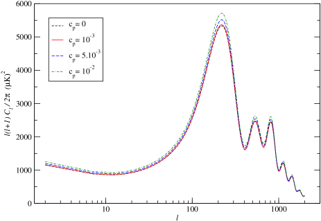
On the other hand, Fig. 15 confirms that varying the moduli coupling constant is not innocuous for the temperature angular power spectrum. However, as previously mentioned, the effective matter field mass is also directly involved in the amplitude of the primordial power spectra through Eq. (23) and one may expect a degeneracy between these parameters on their respective CMB influence. In addition, both and have been shown to modify the tilts of the primordial power spectra in Sect. III.4.
In the next section, a Monte Carlo Markov Chain (MCMC) exploration of the cosmological and primordial parameter space if performed by using the first year WMAP data. Note that the method we are using relies on a full numerical scheme which does not involve any approximation of the primordial power spectra.
IV.3 MCMC exploration
Following the method of Ref. Lewis and Bridle (2002), we consider a parameter space involving a minimal set of cosmological parameters: the ratio of the sound horizon to the angular diameter distance (related to the reduced Hubble parameter ), the density parameter of baryons and cold dark matter , the optical depth (or the redshift of reionization ); as well as our primordial parameters: , , and . Note that the four primordial parameters fix the overall and relative amplitudes of the primordial scalar and tensor power spectra. The MCMC computations have been done by using the cosmomc code Lewis and Bridle (2002) calling the modified camb version based on our inflationary code, and given the first year WMAP data and the associated likelihood code Kogut et al. (2003); Verde et al. (2003); Hinshaw et al. (2003).
In order to check the relevance of our full numerical approach, we have first performed a MCMC exploration on the single field chaotic inflation model which is obtained by fixing . Indeed, the current constraints on the cosmological parameters using the WMAP data usually assume either power law or slow-roll approximated primordial power spectra Peiris et al. (2003); Barger et al. (2003); Leach and Liddle (2003). Since our method goes further it may be interesting to check its consistency with the current existing bounds. Moreover, the single field chaotic model will be our reference model to discuss the more complex features associated with the boundary inflation model.
IV.3.1 Chaotic model
We have used standard prior distributions for the base cosmological parameters (see Ref. Lewis and Bridle (2002)) whereas wide top hat priors have been chosen for the chaotic model parameters: , and . The lower limit on the initial matter field value is set in order to get the right order or magnitude of the minimal total number of efolds required to solve the flatness and homogeneity problem (). In addition, in the cosmomc code, we have coded a “hard prior” rejecting any model for which observable perturbations cannot be initially set in a Bunch-Davies vacuum with : for the chaotic model this can occur when there is not enough efolds of inflation [see Eq. (84)]. The higher limit has been chosen in order to avoid prohibitive computation time which occurs when the total number of efolding become very large. The prior on is chosen to contain the value required to get the right amplitude of the CMB anisotropies. The obtained posterior probability distributions for the base and derived cosmological, as well as the primordial parameters are plotted in Fig. 16 and Fig. 17. They correspond to samples for which the errors on their shape do not exceed . Note that they do not rely on any slow-roll approximation but only on the linear perturbation theory and the cosmological setup of Sect. IV.1.
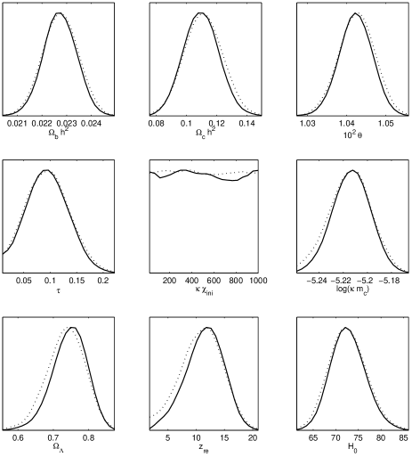
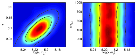
Firstly, the constraints on the base cosmological parameters are found to be consistent with the current state of the art Spergel et al. (2003); Peiris et al. (2003); Leach and Liddle (2003); Tegmark et al. (2004). For the chaotic model parameters, the inflaton mass is well constrained, as expected from a parameter involved in the normalization of the primordial power spectra, and we find, at level
| (102) |
As expected, the initial value of the field is found to be unconstrained. Concerning the overall ability of the chaotic model to fit the data, the best fit is obtained with a likelihood of for degrees of freedom which render the chaotic model slightly more favored than its slow-roll approximated version.
In the next section, a MCMC exploration is performed for the boundary inflation model. Since in the limit this model matches with the chaotic one, the posterior probability distribution of the coupling constant traces how favored or disfavored the boundary inflation model is with respect to the single field chaotic model.
IV.3.2 Boundary inflation model
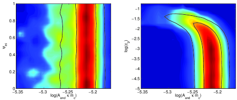
The full set of primordial parameters is now considered: , , and . Compared to the chaotic model, there are two additional parameters and , and a rescaled one: . Remember that the latter no longer refers to the bare mass of the matter field but to its effective mass at the end of inflation. A flat prior has been chosen for the moduli coupling constant: . The lower limit corresponds to the decoupling between the and fields for which the boundary model is equivalent to single field chaotic inflation, whereas the upper limit correspond to the weak post-inflationary bound above which the moduli influence the late-time cosmology (see Sect. IV.1). Concerning the values, we have set a conservative top hat prior since, according to our prescription, larger values of cannot be observed from the CMB point of view (see Sect. III.2.4). The other priors for the base cosmological parameters and the effective mass are the same as for the chaotic model. Their corresponding posterior distributions have been obtained for samples and are plotted in Fig. 18 and Fig. 19 where the marginalized distributions obtained for the chaotic model are also superimposed (red dashed lines).
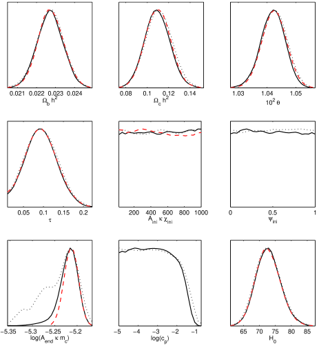
On one hand, the robustness of the cosmological parameters with respect to the primordial power spectra is recovered: there are no significant deviations between their posterior probability distributions in the chaotic model and in the boundary inflation model.
On the other hand, we did not find a better fit of the WMAP data with the boundary inflation primordial power spectra. More precisely, the best fit has the same likelihood than the one obtained with the chaotic model: but now for degrees of freedom. Statistically, the boundary inflation model is disfavored by its additional two parameters which do not help to improve the fit Lewis and Bridle (2002); Lazarides et al. (2004); Trotta (2005). As expected from the previous discussions, the initial values of the background fields and have not observable effect and are consequently unconstrained by the data. Furthermore, the marginalised probability distribution of the coupling constant in Fig. 18 exhibits a plateau for . Since in the decoupling limit the boundary model identifies with the single field chaotic model, the existence of such a plateau shows that the WMAP data are not sensitive to the deviation induced by the moduli during inflation as long as . As a result, from the data point of view, all these inflationary models, boundary and chaotic, cannot being distinguished in that regime.
However, the rapid decay of the marginalised probability distribution for values larger than signals the sensitivity of the data in this regime, which disfavour the corresponding boundary inflation models. More precisely, one obtains the two-sigma level upper bound for the moduli coupling constant
| (103) |
which can be recast to an upper limit for the scalar-tensor conformal gradient
| (104) |
at confidence level. In terms of the post-Newtonian parameters more commonly used to constrain scalar-tensor theories Will (2001), we have
| (105) |
In fact, this constraint comes from the effects discussed in Sect. III.4: the tilt of the primordial power spectra in the boundary model increases with the value of the the moduli coupling constant due to the running of the effective matter field mass. Since the WMAP data are compatible with flat primordial power spectra, it is therefore not surprising that they end up constraining deviations from scale-invariance. This effect also explains why the marginalised probability distribution of the effective mass is skewed to lower values. For a given value of , larger values of implies a more efficient running of the conformal factor during inflation, and in particular larger values of at the time when the observable perturbations have left the Hubble radius (see Fig. 11 and Fig. 12). This degeneracy between and is clearly seen in Fig. 19: the two-dimensional marginal probability is distorted in such a way that the overall amplitude of the primordial perturbations fit with the one measured by WMAP.
Let us emphasize again that Eq. (104) holds at the time of inflation and comes only from the shape of the primordial power spectra. In fact, for a given matter sector, this bound certainly applies to any inflationary scalar-tensor models involving a running conformal factor during the generation of primordial perturbations. On the contrary, scalar-tensor models exhibiting a relaxation mechanism toward General Relativity are expected to evade this bound: as it is the case for the moduli in our setup, such scalar gravity fields would reach the minimum of the potential after only a few efolds of inflation thereby freezing the running of the conformal factor. In any case, comparing Eq. (104) to the current solar-system and astrophysical bounds in Eqs. (97) and (99) shows that scalar-tensor inflation should be considered in the search of scalar-tensor effects in cosmology.
V Conclusion
In this paper, we have studied the CMB signatures a minimal realistic boundary inflation model may have in a (reasonably) restricted parameter space in which the observable effects come only from the shapes of the primordial scalar and tensor power spectra.
Firstly, it has been shown that the background evolution involves three different eras corresponding to the domination of one of the three fields over the others. According to the values of the coupling constants, these eras may or may not be of inflationary kind. In our case, one of the moduli field, namely , is associated to a non-accelerated expansion during which it rapidly relaxes toward vanishing values. Once trapped into its minimum, two smoothly connected inflationary periods driven by the moduli and the matter field take place until the matter field oscillates around the minimum of its potential thereby starting a reheating period.
At the perturbation level, we have discussed the generation and observability of the primordial cosmological perturbations arising during these inflationary eras. Since the -dominated era precedes the inflationary eras, this field has not significant observable effects. Moreover, the existence of an attractor in the background fields evolution during inflation erases any memory of the initial conditions when one is concerned with the observable perturbations. As a result, only the effective mass of the matter field and the moduli coupling constant end up being of observable interest for the CMB. The former encodes the amplitude of the primordial perturbations at Hubble exit and the latter quantifies the changing rate of the conformal factor with respect to the evolution of the moduli . Moreover, as expected for a multifield system, there are entropy perturbations which source the adiabatic modes after Hubble exit. However, for cosmologically relevant values of the moduli coupling constant , the entropy and adiabatic modes are found to be weakly coupled and the adiabatic power spectrum dominates at the end of inflation. Nevertheless, even in this regime, the running of the conformal factor at Hubble exit has been shown to significantly increase the tilt of the adiabatic power spectrum.
We have then assumed a toy cosmological framework in order to compute the seeded CMB anisotropies. In this framework, the moduli and survive in the late-time cosmology whereas the standard cosmological fluids are produced by the decay of the matter field . In order to study the observable effects stemming from inflation only, we have focused on values of the moduli coupling constant which do not strongly modify the late-time cosmology, namely . Under this prior choice, we have computed the induced CMB anisotropies and performed a MCMC analysis of the parameter space given the first year WMAP data. The boundary inflation model appears to be indistinguishable from a single field chaotic model as long as whereas it is disfavored for larger values of the coupling constant. Since the overall best fit model lies in the region of the parameter space, the boundary inflation model is statistically disfavored compared to a single chaotic model by its two additional degrees of freedom which do not help to improve the fit. Moreover, the current WMAP data lead to a marginalized probability bound which corresponds to the post-Newtonian Eddington parameter upper limit .
The above bound is not competitive with the solar-system upper limit and remains only slightly stronger than the late-time cosmological one. However, it holds at the time of inflation and provides in this respect a very early constraint to the scalar-tensor models which would behave during inflation as the boundary model, but would relax toward General Relativity afterwards. A word of caution is in order since this constraint certainly does not apply to all scalar-tensor inflationary models. Indeed, it essentially relies on the running of the conformal factor during the generation of the primordial perturbations, and also depends on the shape of the matter potential. For example, one may imagine to freeze the running of the conformal factor by stabilising the moduli in their bulk potential [see Eq. (5)]. However, in view of the future more accurate data, this work suggests that a fully consistent derivation of scalar-tensor theory bounds in the context of cosmology should involve both an inflationary and post-inflationary modelisation of the expected deviations from General Relativity.
The present work has been focused on the inflationary eras only and for simplicity we have not considered reheating phenomena that might modify the evolution of the cosmological perturbations. It could be interesting in future works to quantify these effects in view of the CMB data. In addition, we have not considered the post-inflationary scalar-tensor effects. A natural extension of the current work would be to perform a MCMC exploration on the moduli coupling constants by using simultaneously scalar-tensor inflationary and post-inflationary codes to compute the cosmological perturbations. In particular, one could quantify the late-time effects of the entropy perturbations existing generically between the moduli and the cosmological fluids in such brane world scenarios.
Acknowledgements.
We thank Nicole Audiffren, Carlo Contaldi, Gilles Esposito-Farèse, Samuel Leach, Jérôme Martin, Christophe Rhodes, Roberto Trotta and Jean-Philippe Uzan for enlightening discussions and advices on the different parts of this work. The computations have been performed for one part in the Centre Informatique National de l’Enseignement Supérieur cin during one CPU-time year, and for the other thanks to a substantial time allocation by the French data processing center for Planck-HFI pla and by the U. K. Computational Cosmology Consortium cos . This work is supported in part by PPARC.References
- Eidelman et al. (2004) S. Eidelman, K. Hayes, K. Olive, M. Aguilar-Benitez, C. Amsler, D. Asner, K. Babu, R. Barnett, J. Beringer, P. Burchat, et al., Physics Letters B 592, 1+ (2004), URL http://pdg.lbl.gov.
- Nordström (1914) G. Nordström, Phys. Zeitschr. 15, 504 (1914).
- Kaluza (1921) T. Kaluza, Sitzungsber. Preuss. Akad. Wiss. Berlin p. 966 (1921).
- Klein (1926) O. Klein, Z. Phys. 37, 895 (1926).
- O’Raifeartaigh and Straumann (2000) L. O’Raifeartaigh and N. Straumann, Rev. Mod. Phys 72, 1 (2000).
- Polchinski (1998a) J. Polchinski, String theory. An introduction to the bosonic string, Vol. I (Cambridge University Press, Cambridge, UK, 1998a).
- Polchinski (1998b) J. Polchinski, String theory. Superstring theory and beyond, Vol. II (Cambridge University Press, Cambridge, UK, 1998b).
- Horava and Witten (1996) P. Horava and E. Witten, Nucl. Phys. B475, 94 (1996), eprint hep-th/9603142.
- Witten (1996) E. Witten, Nucl. Phys. B471, 135 (1996), eprint hep-th/9602070.
- Langlois (2003) D. Langlois, Prog. Theor. Phys. Suppl. 148, 181 (2003), eprint hep-th/0209261.
- Maartens (2004) R. Maartens, Living Rev. Rel. 7, 7 (2004), eprint gr-qc/0312059.
- Brax et al. (2004) P. Brax, C. van de Bruck, and A.-C. Davis, Rept. Prog. Phys. 67, 2183 (2004), eprint hep-th/0404011.
- Akama (1982) K. Akama, Lect. Notes Phys. 176, 267 (1982), eprint hep-th/0001113.
- Rubakov and Shaposhnikov (1983) V. A. Rubakov and M. E. Shaposhnikov, Phys. Lett. B125, 136 (1983).
- Davis et al. (2001) A.-C. Davis, S. C. Davis, W. B. Perkins, and I. R. Vernon, Phys. Lett. B504, 254 (2001), eprint hep-ph/0008132.
- Battye and Carter (1995) R. A. Battye and B. Carter, Phys. Lett. B357, 29 (1995), eprint hep-ph/9508300.
- Battye et al. (2001) R. A. Battye, B. Carter, A. Mennim, and J.-P. Uzan, Phys. Rev. D64, 124007 (2001), eprint hep-th/0105091.
- Binetruy et al. (2000) P. Binetruy, C. Deffayet, and D. Langlois, Nucl. Phys. B565, 269 (2000), eprint [http://arXiv.org/abs]hep-th/9905012.
- Maartens et al. (2000) R. Maartens, D. Wands, B. A. Bassett, and I. Heard, Phys. Rev. D62, 041301 (2000), eprint hep-ph/9912464.
- Randall and Sundrum (1999a) L. Randall and R. Sundrum, Phys. Rev. Lett. 83, 4690 (1999a), eprint hep-th/9906064.
- Randall and Sundrum (1999b) L. Randall and R. Sundrum, Phys. Rev. Lett. 83, 3370 (1999b), eprint hep-ph/9905221.
- Garriga and Tanaka (2000) J. Garriga and T. Tanaka, Phys. Rev. Lett. 84, 2778 (2000), eprint hep-th/9911055.
- Arkani-Hamed et al. (1998) N. Arkani-Hamed, S. Dimopoulos, and G. R. Dvali, Phys. Lett. B429, 263 (1998), eprint hep-ph/9803315.
- Antoniadis et al. (1998) I. Antoniadis, N. Arkani-Hamed, S. Dimopoulos, and G. R. Dvali, Phys. Lett. B436, 257 (1998), eprint hep-ph/9804398.
- Ringeval et al. (2003) C. Ringeval, T. Boehm, and R. Durrer (2003), eprint hep-th/0307100.
- Dvali et al. (2000) G. R. Dvali, G. Gabadadze, and M. Porrati, Phys. Lett. B485, 208 (2000), eprint hep-th/0005016.
- Antoniadis et al. (2003) I. Antoniadis, R. Minasian, and P. Vanhove, Nucl. Phys. B648, 69 (2003), eprint hep-th/0209030.
- Cremades et al. (2002) D. Cremades, L. E. Ibanez, and F. Marchesano, Nucl. Phys. B643, 93 (2002), eprint hep-th/0205074.
- Kokorelis (2004) C. Kokorelis, Nucl. Phys. B677, 115 (2004), eprint hep-th/0207234.
- Kohlprath (2004) E. Kohlprath, Nucl. Phys. B697, 243 (2004), eprint hep-th/0311251.
- Kolanovic et al. (2003) M. Kolanovic, M. Porrati, and J.-W. Rombouts, Phys. Rev. D68, 064018 (2003), eprint hep-th/0304148.
- Ringeval and Rombouts (2005) C. Ringeval and J.-W. Rombouts, Phys. Rev. D71, 044001 (2005), eprint hep-th/0411282.
- Cvetic and Soleng (1997) M. Cvetic and H. H. Soleng, Phys. Rept. 282, 159 (1997), eprint hep-th/9604090.
- Bonjour et al. (1999) F. Bonjour, C. Charmousis, and R. Gregory, Class. Quant. Grav. 16, 2427 (1999), eprint gr-qc/9902081.
- Antunes et al. (2002) N. D. Antunes, E. J. Copeland, M. Hindmarsh, and A. Lukas (2002), eprint hep-th/0208219.
- Ringeval et al. (2005) C. Ringeval, P. Peter, and J.-P. Uzan, Phys. Rev. D71, 104018 (2005), eprint hep-th/0301172.
- Koyama et al. (2004) K. Koyama, D. Langlois, R. Maartens, and D. Wands, JCAP 0411, 002 (2004), eprint hep-th/0408222.
- Cartier and Durrer (2005) C. Cartier and R. Durrer, Phys. Rev. D71, 064022 (2005), eprint hep-th/0409287.
- Lukas et al. (2000) A. Lukas, B. A. Ovrut, and D. Waldram, Phys. Rev. D61, 023506 (2000), eprint hep-th/9902071.
- Lukas et al. (1999) A. Lukas, B. A. Ovrut, K. S. Stelle, and D. Waldram, Nucl. Phys. B552, 246 (1999), eprint hep-th/9806051.
- Brax and Davis (2001) P. Brax and A. C. Davis, Phys. Lett. B497, 289 (2001), eprint hep-th/0011045.
- Ashcroft et al. (2004a) P. R. Ashcroft, C. van de Bruck, and A. C. Davis, Phys. Rev. D69, 083516 (2004a), eprint astro-ph/0210597.
- Brax et al. (2003a) P. Brax, C. van de Bruck, A. C. Davis, and C. S. Rhodes, Phys. Rev. D67, 023512 (2003a), eprint hep-th/0209158.
- Kobayashi and Koyama (2002) S. Kobayashi and K. Koyama, JHEP 12, 056 (2002), eprint hep-th/0210029.
- Brax et al. (2003b) P. Brax, C. van de Bruck, A. C. Davis, and C. S. Rhodes (2003b), eprint hep-ph/0309180.
- Ashcroft et al. (2004b) P. R. Ashcroft, C. van de Bruck, and A. C. Davis, Phys. Rev. D69, 063519 (2004b), eprint astro-ph/0310643.
- Kanno and Soda (2004) S. Kanno and J. Soda, Gen. Rel. Grav. 36, 689 (2004), eprint hep-th/0303203.
- Palma and Davis (2004a) G. A. Palma and A.-C. Davis, Phys. Rev. D70, 064021 (2004a), eprint hep-th/0406091.
- Davis et al. (2005) A. C. Davis, P. Brax, and C. van de Bruck, Nucl. Phys. Proc. Suppl. 148, 64 (2005), eprint astro-ph/0503467.
- Damour and Esposito-Farese (1992) T. Damour and G. Esposito-Farese, Class. Quant. Grav. 9, 2093 (1992).
- Will (2001) C. M. Will, Living Rev. Rel. 4, 4 (2001), eprint gr-qc/0103036.
- Damour and Pichon (1999) T. Damour and B. Pichon, Phys. Rev. D59, 123502 (1999), eprint astro-ph/9807176.
- Perrotta et al. (2000) F. Perrotta, C. Baccigalupi, and S. Matarrese, Phys. Rev. D61, 023507 (2000), eprint astro-ph/9906066.
- Chen and Kamionkowski (1999) X.-l. Chen and M. Kamionkowski, Phys. Rev. D60, 104036 (1999), eprint astro-ph/9905368.
- Baccigalupi et al. (2000) C. Baccigalupi, S. Matarrese, and F. Perrotta, Phys. Rev. D62, 123510 (2000), eprint astro-ph/0005543.
- Amendola (2001) L. Amendola, Phys. Rev. Lett. 86, 196 (2001), eprint astro-ph/0006300.
- Riazuelo and Uzan (2002) A. Riazuelo and J.-P. Uzan, Phys. Rev. D66, 023525 (2002), eprint astro-ph/0107386.
- Nagata et al. (2004) R. Nagata, T. Chiba, and N. Sugiyama, Phys. Rev. D69, 083512 (2004), eprint astro-ph/0311274.
- Acquaviva et al. (2005) V. Acquaviva, C. Baccigalupi, S. M. Leach, A. R. Liddle, and F. Perrotta, Phys. Rev. D71, 104025 (2005), eprint astro-ph/0412052.
- Esposito-Farese (2004) G. Esposito-Farese (2004), eprint gr-qc/0402007.
- Uzan (2005) J.-P. Uzan, AIP Conf. Proc. 736, 3 (2005), eprint astro-ph/0409424.
- Schimd et al. (2005) C. Schimd, J.-P. Uzan, and A. Riazuelo, Phys. Rev. D71, 083512 (2005), eprint astro-ph/0412120.
- Rhodes et al. (2003) C. S. Rhodes, C. van de Bruck, P. Brax, and A. C. Davis, Phys. Rev. D68, 083511 (2003), eprint astro-ph/0306343.
- Damour and Nordtvedt (1993) T. Damour and K. Nordtvedt, Phys. Rev. D48, 3436 (1993).
- Kogut et al. (2003) A. Kogut et al., Astrophys. J. Suppl. 148, 161 (2003), eprint astro-ph/0302213.
- Verde et al. (2003) L. Verde et al., Astrophys. J. Suppl. 148, 195 (2003), eprint astro-ph/0302218.
- Hinshaw et al. (2003) G. Hinshaw et al., Astrophys. J. Suppl. 148, 135 (2003), eprint astro-ph/0302217.
- Palma and Davis (2004b) G. A. Palma and A.-C. Davis, Phys. Rev. D70, 106003 (2004b), eprint hep-th/0407036.
- Lewis et al. (2000) A. Lewis, A. Challinor, and A. Lasenby, Astrophys. J. 538, 473 (2000), eprint astro-ph/9911177.
- Lewis and Bridle (2002) A. Lewis and S. Bridle, Phys. Rev. D66, 103511 (2002), eprint astro-ph/0205436.
- Kofman et al. (2004) L. Kofman et al., JHEP 05, 030 (2004), eprint hep-th/0403001.
- Koshelev (2004) N. A. Koshelev, Grav. Cosmol. 10, 289 (2004), eprint astro-ph/0501600.
- Collins (1971) C. B. Collins, Commun. Math. Phys. 23, 137 (1971).
- Collins (1972) C. B. Collins, Commun. Math. Phys. 27, 37 (1972).
- Shikin (1973) I. S. Shikin, Sov. Phys. JETP 36, 811 (1973).
- Gordon et al. (2001) C. Gordon, D. Wands, B. A. Bassett, and R. Maartens, Phys. Rev. D63, 023506 (2001), eprint astro-ph/0009131.
- Di Marco et al. (2003) F. Di Marco, F. Finelli, and R. Brandenberger, Phys. Rev. D67, 063512 (2003), eprint astro-ph/0211276.
- Esposito-Farese and Polarski (2001) G. Esposito-Farese and D. Polarski, Phys. Rev. D63, 063504 (2001), eprint gr-qc/0009034.
- Linde (2001) A. Linde, JHEP 11, 052 (2001), eprint hep-th/0110195.
- Noh and Hwang (2001) H. Noh and J.-c. Hwang, Phys. Lett. B515, 231 (2001), eprint astro-ph/0107069.
- Di Marco and Finelli (2005) F. Di Marco and F. Finelli, Phys. Rev. D71, 123502 (2005), eprint astro-ph/0505198.
- Martin (2004) J. Martin (2004), eprint hep-th/0406011.
- Turner (1983) M. S. Turner, Phys. Rev. D28, 1243 (1983).
- Shtanov et al. (1995) Y. Shtanov, J. H. Traschen, and R. H. Brandenberger, Phys. Rev. D51, 5438 (1995), eprint hep-ph/9407247.
- Kofman et al. (1997) L. Kofman, A. D. Linde, and A. A. Starobinsky, Phys. Rev. D56, 3258 (1997), eprint hep-ph/9704452.
- Groot Nibbelink and van Tent (2002) S. Groot Nibbelink and B. J. W. van Tent, Class. Quant. Grav. 19, 613 (2002), eprint hep-ph/0107272.
- Hwang and Noh (2002) J.-c. Hwang and H. Noh, Class. Quant. Grav. 19, 527 (2002), eprint astro-ph/0103244.
- Lukash (1980) V. N. Lukash, Sov. Phys. JETP 52, 807 (1980).
- Lyth (1985) D. H. Lyth, Phys. Rev. D31, 1792 (1985).
- Kodama and Sasaki (1984) H. Kodama and M. Sasaki, Prog. Theor. Phys. Suppl. 78, 1 (1984).
- Mukhanov et al. (1992) V. F. Mukhanov, H. A. Feldman, and R. H. Brandenberger, Phys. Rept. 215, 203 (1992).
- Durrer (1994) R. Durrer, Fundamentals of Cosmic Physics 15,3, 209 (1994), eprint [http://arXiv.org/abs]astro-ph/9311041.
- Martin and Schwarz (1998) J. Martin and D. J. Schwarz, Phys. Rev. D57, 3302 (1998), eprint gr-qc/9704049.
- Carter (1997) B. Carter (1997), eprint hep-th/9705172.
- Langlois (1999) D. Langlois, Phys. Rev. D59, 123512 (1999), eprint astro-ph/9906080.
- Salopek et al. (1989) D. S. Salopek, J. R. Bond, and J. M. Bardeen, Phys. Rev. D40, 1753 (1989).
- Tsujikawa et al. (2003) S. Tsujikawa, D. Parkinson, and B. A. Bassett, Phys. Rev. D67, 083516 (2003), eprint astro-ph/0210322.
- Martin and Ringeval (2004) J. Martin and C. Ringeval, Phys. Rev. D69, 083515 (2004), eprint astro-ph/0310382.
- Easther et al. (2005) R. Easther, W. H. Kinney, and H. Peiris (2005), eprint astro-ph/0505426.
- Kaloper et al. (2002) N. Kaloper, M. Kleban, A. Lawrence, S. Shenker, and L. Susskind, JHEP 11, 037 (2002), eprint hep-th/0209231.
- Martin and Brandenberger (2003) J. Martin and R. Brandenberger, Phys. Rev. D68, 063513 (2003), eprint hep-th/0305161.
- Liddle and Lyth (1993) A. R. Liddle and D. H. Lyth, Phys. Rept. 231, 1 (1993), eprint astro-ph/9303019.
- Adams et al. (1997) J. A. Adams, G. G. Ross, and S. Sarkar, Nucl. Phys. B503, 405 (1997), eprint hep-ph/9704286.
- Kaloper and Kaplinghat (2003) N. Kaloper and M. Kaplinghat, Phys. Rev. D68, 123522 (2003), eprint hep-th/0307016.
- Hunt and Sarkar (2004) P. Hunt and S. Sarkar, Phys. Rev. D70, 103518 (2004), eprint astro-ph/0408138.
- Martin and Schwarz (2000) J. Martin and D. J. Schwarz, Phys. Rev. D62, 103520 (2000), eprint astro-ph/9911225.
- Starobinsky and Yokoyama (1994) A. A. Starobinsky and J. Yokoyama (1994), eprint gr-qc/9502002.
- Garcia-Bellido and Wands (1995) J. Garcia-Bellido and D. Wands, Phys. Rev. D52, 6739 (1995), eprint gr-qc/9506050.
- Liddle and Leach (2003) A. R. Liddle and S. M. Leach, Phys. Rev. D68, 103503 (2003), eprint astro-ph/0305263.
- Bertotti et al. (2003) B. Bertotti, L. Iess, and P. Tortora, Nature 425, 374 (2003).
- Williams et al. (1996) J. G. Williams, X. X. Newhall, and J. O. Dickey, Phys. Rev. D53, 6730 (1996).
- Tegmark and Zaldarriaga (2002) M. Tegmark and M. Zaldarriaga, Phys. Rev. D66, 103508 (2002), eprint astro-ph/0207047.
- Peiris et al. (2003) H. V. Peiris et al., Astrophys. J. Suppl. 148, 213 (2003), eprint astro-ph/0302225.
- Leach and Liddle (2003) S. M. Leach and A. R. Liddle, Phys. Rev. D68, 123508 (2003), eprint astro-ph/0306305.
- Barger et al. (2003) V. Barger, H.-S. Lee, and D. Marfatia, Phys. Lett. B565, 33 (2003), eprint hep-ph/0302150.
- Bond et al. (2004) J. R. Bond, C. R. Contaldi, A. M. Lewis, and D. Pogosyan, Int. J. Theor. Phys. 43, 599 (2004), eprint astro-ph/0406195.
- Leach (2005) S. Leach (2005), eprint astro-ph/0506390.
- Spergel et al. (2003) D. N. Spergel et al. (WMAP), Astrophys. J. Suppl. 148, 175 (2003), eprint astro-ph/0302209.
- Tegmark et al. (2004) M. Tegmark et al. (SDSS), Phys. Rev. D69, 103501 (2004), eprint astro-ph/0310723.
- Lazarides et al. (2004) G. Lazarides, R. R. de Austri, and R. Trotta, Phys. Rev. D70, 123527 (2004), eprint hep-ph/0409335.
- Trotta (2005) R. Trotta (2005), eprint astro-ph/0504022.
- (122) URL http://www.cines.fr.
- (123) URL http://www.planck.fr.
- (124) URL http://www.damtp.cam.ac.uk/cosmos.