Oxygen and Nitrogen in Leo A and GR 8

Abstract

We present elemental abundances for multiple HII regions in Leo A and GR 8 obtained from long slit optical spectroscopy of these two nearby low luminosity dwarf irregular galaxies. As expected from their luminosities, and in agreement with previous observations, the derived oxygen abundances are extremely low in both galaxies. High signal-to-noise ratio observations of a planetary nebula in Leo A yield 12 + log(O/H) = 7.30 $\pm$ 0.05; “semi-empirical” calculations of the oxygen abundance in four HII regions in Leo A indicate 12 + log(O/H) = 7.38 $\pm$ 0.10. These results confirm that Leo A has one of the lowest ISM metal abundances of known nearby galaxies. Based on results from two HII regions with high signal-to-noise measurements of the weak [O III] $\lambda$4363 line, the mean oxygen abundance of GR 8 is 12 + log(O/H) = 7.65 $\pm$ 0.06; using “empirical” and “semi-empirical” methods, similar abundances are derived for 6 other GR 8 HII regions. Similar to previous results in other low metallicity galaxies, the mean log(N/O) $=$ $-$1.53 $\pm$ 0.09 for Leo A and $-$1.51 $\pm$ 0.07 for GR 8. There is no evidence of significant variations in either O/H or N/O in the HII regions. The metallicity-luminosity relation for nearby (D $<$ 5 Mpc) dwarf irregular galaxies with measured oxygen abundances has a mean correlation of 12 + log(O/H) = 5.67 $-$ 0.151 M_B with a dispersion in oxygen about the relationship of $\sigma$ $=$ 0.21. These observations confirm that gas-rich low luminosity galaxies have extremely low elemental abundances in the ionized gas-phase of their interstellar media. Although Leo A has one of the lowest metal abundances of known nearby galaxies, detection of tracers of an older stellar population (RR Lyrae variable stars, horizontal branch stars, a well populated red giant branch) indicate that it is not a newly formed galaxy as has been proposed for some other similarly low metallicity star forming galaxies.

1 Introduction

Understanding the evolution of dwarf galaxies, and, in particular, the chemical evolution of dwarf galaxies, has implications for our understanding of important processes in galaxy evolution, stellar nucleosynthesis, and the enrichment of the intergalactic medium. While a general relationship between galaxy luminosity and current metallicity has been well established for all galaxies, the fundamental underlying process (or processes) is still debated. The star formation histories of dwarf galaxies are also far from well understood. Is it possible for dwarf galaxies to form in the current epoch, or are the identities of all dwarf galaxies established at early times? Can massive star formation result in the instantaneous enrichment of the interstellar medium of a dwarf galaxy, or is the bulk of the newly synthesized heavy elements released into a coronal gas phase which must cool before becoming incorporated into the other phases of the ISM and eventually the next generation of stars? By studying extreme dwarf irregular galaxies, i.e., the lowest luminosity, lowest metallicity and lowest mass star forming systems, we can extend the baseline for comparative studies of galaxies and test simple hypotheses of the formation of dwarf galaxies. This is particularly important for studying the chemical evolution of dwarf galaxies, as the impact of a given episode of star formation on a dwarf galaxy will be maximal for the lowest luminosity and metallicity systems. In principle, this could lead to the largest deviations from the luminosity-metallicity relationship, and this, in turn, may lead to a better understanding of that relationship.

Gas phase abundances are one of the best measures of the intrinsic metallicity of low mass galaxies. Here, we present new optical spectroscopy of Leo A and GR 8, two extremely low metallicity dwarf irregular galaxies in the Local Group (see van den Bergh, 2000). Comparable nearby low luminosity galaxies include DDO 210 (no usable HII regions, van Zee et al., 1997a), Sag DIG (empirical O/H only, Skillman, Terlevich, & Melnick, 1989; Saviane et al., 2002; Lee, Grebel & Hodge, 2003), and Peg DIG (faint HII regions with no detectable [O III] emission, Skillman, Bomans, & Kobulnicky (1997)). These (and other) observations indicate that it is often difficult to measure the gas-phase abundance of low luminosity galaxies simply because there are few bright HII regions. Thus, accurate oxygen abundance measurements of multiple HII regions in Leo A and GR 8 have the potential to substantially further our understanding of chemical enrichment and mixing of enriched material in low mass galaxies.

A summary of select global parameters of Leo A and GR 8 is presented in Table 1. At a distance of only 690 kpc, Leo A may be the nearest low metallicity star forming galaxy. Observations of the resolved stellar population in Leo A indicate an extremely low metallicity ($\sim$ 3% of solar) for even the youngest stars (Tolstoy et al., 1998). However, accurate gas phase metallicities have been difficult to obtain for this system, in part due to the low surface brightnesses of the faint HII regions. The one exception is the bright planetary nebula (PN) in the northeastern quadrant of the galaxy. An oxygen abundance of $\sim$ 2% of the solar value was derived from observations of this planetary nebula (Skillman et al., 1989), but it was never certain if this value was representative of the galaxy as a whole, or just the gas ionized by the PN. We thus set out to observe several of the HII regions in Leo A in order to obtain a more representative estimate of the gas phase oxygen abundance.

GR 8 is slightly more luminous and metal–rich than Leo A, but it is also an extremely low metallicity system. Previous oxygen abundance measurements indicate that GR 8 has an oxygen abundance of approximately 5% of the solar value (Skillman et al., 1988; Moles et al., 1990). However, an unusually high N/O ratio derived for one of the HII regions suggested that there might be regions of local nitrogen enrichment (Moles et al., 1990). We thus decided to observe several HII regions in GR 8 to determine if there are regions of local nitrogen enrichment in this low mass galaxy.

This paper is organized as follows. In §2 we present spectroscopic observations of Leo A and GR 8. In §3 we present the nebular abundance calculations and discuss direct and strong line abundance calibrations. In §4 we compare the abundance determinations of these two low luminosity galaxies to values for other galaxies in the literature. In §5 we demonstrate that even though Leo A and GR 8 are among the lowest metallicity systems known, observations of resolved stars in these galaxies indicate that star formation in these galaxies has occurred across the age of the universe.

2 Observations

2.1 Optical Spectroscopy

Long slit optical spectra of GR 8 and Leo A were obtained with the Double Spectrograph on the 5m Palomar telescope on the nights of 18 and 19 February 1999. The observations were obtained in long–slit mode; the 2′ long–slit was set to an aperture 2″ wide. Complete spectral coverage from 3600–7600 Å was obtained by using a 5500 Å dichroic to split the light to the two sides (blue and red) of the spectrograph. The blue side was equipped with a 600 l/mm grating; the red side was equipped with a 300 l/mm grating. The effective spectral resolutions were well matched between the two sides, with a resolution of 5.0 Å (1.72 Å pix^-1) on the blue side and 7.9 Å (2.47 Å pix^-1) on the red side. Wavelength calibration was obtained by observations of arc lamps obtained before and after the galaxy observations. A hollow cathode (Fe and Ar) lamp was used to calibrate the blue spectra; a combination of He, Ne, and Ar lamps were used to calibrate the red spectra.

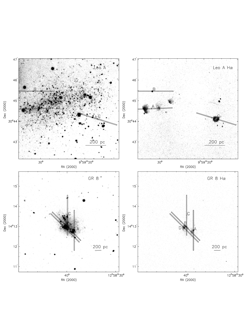
Figure 1: R-band and H$\alpha$ images of Leo A and GR 8 with slit positions marked. The pointings and orientations were optimized to include multiple HII regions while still maintaining a position angle close to the parallactic angle at the time of the observation.

Stellar and HII region coordinates were obtained from H$\alpha$ images kindly provided by E. Tolstoy (Leo A) and J. J. Salzer (GR 8). H$\alpha$ imaging of Leo A has previously been published by Strobel, Hodge, & Kennicutt (1991) (but their field of view did not cover the westernmost HII regions) and Hunter et al. (1993). H$\alpha$ imaging of GR 8 can also be found in Hodge, Lee, & Kennicutt (1989) and references therein. Astrometric plate solutions for these images were calculated using the coordinates of bright stars in the APM catalog (Maddox et al., 1990), yielding positions accurate to within 1″. Optimum slit positions were determined so that the slit could cross several HII regions during each observation while, at the same time, remaining close to the parallactic angle (Figure 1). Due to the faintness of the HII regions, all observations were conducted via blind offsets from nearby stars with typical offsets on the order of 30″ – 80″. The observations were broken into a series of 20 minute exposures; typical observations were sets of 6 or 7 for HII regions in Leo A and sets of 2 or 3 for HII regions in GR 8 (Table 2).

As can be seen in Figure 1, in Leo A, the three slit positions include a mixture of HII region morphologies, while in GR 8 the four slit positions include all major HII regions. Previous Keck 10m observations of the two compact HII regions in the northwest of Leo A and the diffuse HII region located north of slit A indicated that all of these HII regions have weak or non-detectable [O II] and [O III] emission (H. A. Kobulnicky, private communication). Thus, the present observations concentrate on diffuse HII regions in Leo A, including the ring-like structure to the southwest (slit C), as well as observations of the planetary nebula (slit B). The HII region observations also serendipitously included one background galaxy in each field. Observations of the compact HII region south of slit C of Leo A were obtained on 23 January 1999 under very cloudy conditions; while these observations are not discussed here since the target HII region was only marginally detected (due to the clouds), this slit orientation included the background spiral galaxy at 09:59:15.85, 30:43:46.1 (J2000) with z = 0.1467 $\pm$ 0.0002. Finally, slit C of GR 8 included the background spiral galaxy at 12:58:39.95, 14:14:25.7 (J2000), with z = 0.0642 $\pm$ 0.0002.

The spectra were reduced and analyzed with the IRAF package. Spectral reduction followed standard practice including bias subtraction, scattered light corrections, and flat fielding based on both twilight and dome flats. The 2–dimensional (2-d) images were rectified based on the arc lamp observations and the trace of stars at different positions along the slit. Multiple exposures were averaged together after the transformation. The sky background was removed from the 2-d images by fitting a low order polynomial along each column of the spectra. One dimensional (1-d) spectra of the HII regions were then extracted from the images. The 1-d spectra were corrected for atmospheric extinction and flux calibrated based on observations of standard stars from the list of Oke (1990); while the nights were not photometric, the relative line strengths should be robust.

Representative spectra for Leo A and GR 8 are shown in Figures 2 and 3, respectively. Note the excellent agreement in the continuum level in the blue and red spectra which confirms that the extraction regions were well matched on the two cameras. The HII regions in Leo A are generally low excitation, with weak [O III] lines and moderate strength [O II] lines. The one exception is the spectrum of the planetary nebula (+089+031) which has strong [O III] and extremely weak [O II] lines. The weak [N II] and [S II] lines in these spectra clearly indicate that the HII regions in Leo A have low elemental abundances. The HII regions in GR 8 show higher excitation ([O III]/[O II]) than those in Leo A; the [O II] and [O III] lines are strong in all of the GR 8 HII regions. However, similar to Leo A, the weak [NII] and [S II] lines indicate that the HII regions in GR 8 have low elemental abundances.

2.2 Line Intensities

The emission line strengths were measured in the 1-d spectra and then corrected for underlying Balmer absorption and for reddening. Similar to the method described in van Zee et al. (1997a), the strengths of the Balmer emission lines were used to estimate the amount of reddening along the line of sight to each HII region using an iterative technique. The intrinsic Balmer line strengths were interpolated from the tabulated values of Hummer & Storey (1987) for case B recombination, assuming N_e = 100 cm^-3 and T_e = 15000 K. Assuming a value of $R=A_{V}/E_{B-V}=3.1$, the Galactic reddening law of Seaton (1979) as parameterized by Howarth (1983) was adopted to derive the reddening function normalized at H$\beta$. For those HII regions with detected [O III] $\lambda$4363, the temperature was then recalculated from the corrected line strengths and a new reddening coefficient was produced. An underlying Balmer absorption with an equivalent width of 2 Å was assumed in the few instances where the reddening coefficient was significantly different when derived from the observed line ratios of H$\alpha$/H$\beta$ and H$\gamma$/H$\beta$. The reddening coefficients, c_Hβ, derived for each HII region are listed in Tables 3 and 4. These can be compared to the values of the foreground Galactic extinction derived by Schlegel, Finkbeiner, & Davis (1998) of E(B-V) $=$ 0.021 for Leo A and 0.026 for GR 8 which correspond to c(H$\beta$) $=$ 0.03 and 0.04 respectively. These very low values of foreground reddening are less than the errors on all of our reddening measurements. In several instances, the derived reddening coefficients were slightly negative (which is not physical) and in these cases zero reddening was assumed.

The measured intensities of emission lines for the HII regions in Leo A and GR 8 are tabulated in Tables 3 and 4, respectively. The first two columns in these tables give the ionic species and rest wavelength of the transition. The third and subsequent columns list the extinction corrected line intensity relative to H$\beta$ for each detected transition. The H$\beta$ flux and equivalent width for each object are listed at the bottom of the tables; since the nights were non-photometric, the H$\beta$ fluxes should only be taken as indicative values. The error associated with each relative line intensity was determined by taking into account the Poisson noise in the line, the error associated with the sensitivity function, the contributions of the Poisson noise in the continuum, read noise, sky noise, and flat fielding or flux calibration errors, the error in setting the continuum level, assumed to be at the 10% level, and the error in the reddening coefficient. Note that although the spectral coverage of the red camera allows for the measurement of the [O II] $\lambda\lambda$7320,7330 lines, these lines were not detected in any of the spectra due to a combination of intrinsic faintness and strong telluric emission. The spectral coverage of the red camera did not extend to the [S III] $\lambda\lambda$9069,9523 lines.

3 Nebular Abundances

In this section we will derive absolute and relative abundances from the emission line spectra. In order to avoid confusion, we start with an overview of some nomenclature. In those cases where we have detected the temperature sensitive [O III] $\lambda$4363 line, we can calculate abundances following the methods described in Osterbrock (1989), and, following Dinerstein (1990) we will refer to this as the “direct” method. In those cases where [O III] $\lambda$4363 is not observed, but [O III] $\lambda$5007 and [O II] $\lambda$3737 are observed, so-called “empirical” methods can be used to infer oxygen abundances (e.g., Pagel et al., 1979; McGaugh, 1991). van Zee et al. (1997a) has introduced the “semi-empirical” method, which uses the oxygen abundance and ionization parameter implied from photoionization models to infer a consistent electron temperature. That electron temperature can then be used to derive relative abundances with some degree of accuracy since the relative abundances have a much lower sensitivity to the electron temperature than the absolute abundances.

3.1 Direct Abundance Measurements

Direct calculation of the oxygen abundance from the observed [O II] and [O III] emission line strengths is possible if both the electron temperature (T_e) and electron density (N_e) are known. The procedure to calculate T_e and N_e is well described in Osterbrock (1989) and will not be repeated here. A version of the FIVEL program of De Robertis, Dufour, & Hunt (1987) was used to compute T_e and N_e from the reddening–corrected [O III] and [S II] line ratios, respectively. In all cases, the observed [S II] line ratios indicated that the HII regions were within the low density limit (I($\lambda$6716)/I($\lambda$6731) $>$ 1.35). Thus, an N_e of 100 cm^-3 was adopted for all HII regions. Unfortunately, calculating the electron temperature proved to be more difficult since the weak [O III] $\lambda$4363 line was often contaminated by the nearby Hg $\lambda$4358 night sky line. In Leo A, [O III] $\lambda$4363 was detected in only one nebula, which is almost certainly a planetary nebula. While a hint of the [O III] $\lambda$4363 line is visible in several of the GR 8 HII regions (Figure 3), it was only detected solidly in two. Once the electron temperature of the O⁺⁺ ionization zone is derived, the electron temperature of the O⁺ zone is estimated using the approximation given by Pagel et al. (1992). The emissivity coefficients for all of the detected emission lines were then calculated using the FIVEL code (De Robertis, Dufour, & Hunt, 1987).

For all atoms other than oxygen, the derivation of atomic abundances requires the use of ionization correction factors (ICFs) to account for the fraction of each atomic species which is in an unobserved ionization state. To estimate the nitrogen abundance, we assume that N/O = N⁺/O⁺ (Peimbert & Costero, 1969), which is probably accurate to $\pm$20% for O/H $<$ 25% solar (Garnett, 1990). To estimate the neon abundance, we assume that Ne/O = Ne⁺⁺/O⁺⁺ (Peimbert & Costero, 1969). To determine the sulfur and argon abundances, we adopt an ICF from published HII region models to correct for the unobserved S⁺³ and Ar⁺⁴ states (e.g., Thuan et al., 1995). In HII regions where S⁺² $\lambda 6312$ was not detected, we do not calculate a sulfur abundance as the ICF becomes too uncertain (Garnett, 1989).

3.1.1 Leo A +089+031 (PN)

The highest surface brightness feature in the H$\alpha$ image of Leo A is the bright planetary nebula in the northeastern part of the galaxy. Note that the H$\alpha$/H$\beta$ ratio is close to the theoretical value, showing no evidence of the anomaly in the observations of Skillman et al. (1989). The weak [O III] $\lambda$4363 line is clearly detected in the high signal–to–noise spectrum of this region (Figure 2). However, it should be noted that [O II] $\lambda$3727 was not detected in this spectrum, and thus, in principle, the oxygen abundance derived from the [O III] emission (12 + log(O/H) = 7.30 $\pm$ 0.05) is a lower limit (Table 5). However, an upper limit on the [O II] $\lambda$3727 line, listed in Table 3, corresponds to an O⁺/H abundance of less than 4% of the O⁺⁺/H abundance, which is significantly smaller than the error on the total abundance. Thus, we will treat this number as the best estimate of the oxygen abundance, noting that this result is similar to that derived previously for the PN (Skillman et al., 1989) in this low luminosity galaxy. Note that, unfortunately, it is not possible to measure the N/O, S/O, and Ar/O ratios directly in this object because the [O II] $\lambda$3727 was not detected and that is required for the ionization correction schemes for these elements.

3.1.2 GR 8 –019–019 and +008–011

Two of the HII regions in GR 8 have solid [O III] $\lambda$4363 detections. Following the procedure outlined above, the oxygen, nitrogen, neon, sulfur, and argon abundances were calculated for GR 8 –019–019 and +008–011. The electron temperatures derived from the [O III] line ratios are listed in Table 5. The ionic abundances relative to hydrogen were computed using the data listed in Table 4; if more than one line was observed for a given ion, the final ionic abundances were calculated to be the weighted averages of the values for the different lines. The nebular abundances were then calculated based on the ionic abundances and the ICFs as described above. The derived 12 + log(O/H), log(N/O), log(Ne/O), log(S/O), and log(Ar/O) for these HII regions are listed in Table 6. The mean oxygen abundance for these two HII regions is 12 + log(O/H) = 7.65 $\pm$ 0.06, in excellent agreement with previous direct oxygen abundance measurements for GR 8 (12 + log(O/H) = 7.48 $\pm$ 0.14; 7.68, Skillman et al., 1988; Moles et al., 1990).

3.2 Strong Line Oxygen Abundance Measurements

As first discussed by Pagel et al. (1979), the oxygen abundance of an HII region can be estimated from the strong line ratio, R${}_{\rm 23}=$ ([O II] + [O III])/H$\beta$, since this parameter varies smoothly as a function of stellar effective temperature and oxygen abundance. Furthermore, while this ratio is double valued, the degeneracy of the R₂₃ relation can be broken by examining the relative strengths of [N II] and [O II]. If the nitrogen lines are extremely weak, as is the case for both Leo A and GR 8 (Figures 2 and 3), only the lower oxygen abundance branch needs to be considered. However, an additional spread in the estimated oxygen abundance for a given R₂₃ is introduced by the geometry of the HII region (e.g., Skillman, 1989; McGaugh, 1991); geometric effects can be represented by the average ionization parameter, Ū, the ratio of ionizing photon density to particle density. This second parameter can be traced by the ratio of the abundance of atoms in different ionization states. Thus, both the sum of the oxygen lines (R₂₃) and the ratio of [O III] to [O II] need to be considered before an oxygen abundance can be determined from the strong lines. For example, the low abundance branch of the model grid McGaugh (1991) generated for an IMF with an upper mass limit of 60 M_⊙ is shown in Figure 4. In this model (and other similar theoretical abundance calibrations, e.g., Kewley & Dopita 2002), the R₂₃ value and [OIII]/[OII] ratio are used to derive an empirical estimate of the oxygen abundance.

As illustrated in Figure 4, the HII regions in GR 8 cluster around an oxygen abundance of 12 + log(O/H) = 7.8 in the McGaugh (1991) calibration, indicating that all of these HII regions have a similar oxygen abundance. However, there is a troubling discrepancy between the oxygen abundances derived from the McGaugh (1991) calibration and those obtained by direct calculation based on measured T_e and individual line strengths (e.g., Pilyugin, 2000; Pérez-Monero & Díaz, 2005; van Zee & Haynes, 2005). In general, the McGaugh (1991) calibration appears to yield abundances that are systematically 0.1-0.2 dex higher than direct calculations; this discrepancy is also found for the HII regions in GR 8 (direct abundance calculations yield 12 + log(O/H) = 7.65 $\pm$ 0.06, Section 3.1.2).

An alternative empirical calibration scheme was proposed be Pilyugin (2000) based on HII regions where [O III] $\lambda$4363 has been detected (the p-method). The Pilyugin (2000) relations for 12 + log(O/H) between 7.4 and 8.2 are shown in Figure 4. In the high ionization regime (Ū $\sim$ 0.01 – 0.1), the shapes of the McGaugh curves and the Pilyugin relations are reasonably similar, but the Pilyugin relations give oxygen abundances $\sim$ 0.12-0.15 dex lower for the same R₂₃ value. However, as discussed in Skillman, Côté, & Miller (2003) and van Zee & Haynes (2005), and is also clear from Figure 4, the empirical relations of Pilyugin (2000) are only valid in this high ionization regime, where there were sufficient T_e measurements in the literature to enable such a calibration. In the low ionization regime, the regime of most of the HII regions in GR 8 and Leo A, the empirical relations of Pilyugin (2000) clearly deviate from results of photoionization models and physical intuition. Indeed, van Zee & Haynes (2005) demonstrate that the empirical abundances derived from the p-method have a clear systematic offset that correlates with ionization parameter. Thus, the empirical oxygen abundances listed in Table 6 for the HII regions in Leo A and GR 8 are based on the McGaugh (1991) model grid, despite the inherent uncertainties and possible systematic errors. The empirical abundances of Pilyugin (2000) will not be discussed further.

While the GR 8 HII regions clearly outline a common locus in Figure 4, the HII regions in Leo A appear to be more widely scattered in ionization parameter and, perhaps, oxygen abundance. Two of the observed HII regions have extremely low ionization parameters (Leo A +069–018 and +112–020); both are extremely diffuse HII regions located in the eastern half of the galaxy. For +069–018, [O III] $\lambda$5007 is barely detected, indicating that this HII region has an extremely low ionization parameter. Similar low excitation spectra were seen in the faint HII region of another Local Group galaxy, Peg DIG (Skillman, Bomans, & Kobulnicky, 1997). For Peg DIG, the morphology (compact) and spectrum of the HII region is consistent with an ionizing flux of a single B0 star. In Leo A, the Balmer line flux that is observed corresponds to ionization by B0 - O9.5 ZAMS stars for each of the 4 HII regions. It is thus possible that the IMF is truncated (or incompletely sampled) or that these HII regions are evolved (aged). However, unlike Peg DIG, the low excitation HII regions in Leo A are diffuse, amorphous structures; thus, it is also possible that the long slit observations do not sample fully the different ionization zones of these HII regions. In particular, if the observations are missing a significant fraction of the O⁺⁺ ionization zone, these HII regions may be displaced significantly in Figure 4; with additional [O III], their location would shift significantly upwards and slightly to the right, possibly moving them into the same metallicity regime as the other two HII regions.

Nonetheless, since the Balmer line fluxes of the HII regions in Leo A are consistent with radiation from lower mass, cooler O and B stars, we examine further the effect of aging in the abundance diagnostic diagram. In Figure 5 we place the low metallicity models (12 + log(O/H) = 7.33) of Stasińska & Leitherer (1996) in the diagnostic grid of Figure 4. As can be seen in Figure 5, aging of HII regions can introduce significant scatter in the abundance diagnostic diagram as both the ionization parameter and shape of the ionizing spectrum evolve (e.g., Stasińska & Leitherer, 1996; Olofsson, 1997), Thus, once one allows for a large range of ionizing spectra and ionization parameter, HII regions of a single oxygen abundance can populate a large range of positions in this diagnostic diagram. This is further emphasized in the bottom panel of Figure 5 where the positions of theoretical HII regions with the same oxygen abundance as the models in the upper part of the Figure are shown with varying values of the electron temperature and ionic fraction.

While the results of Figure 5 may appear to suggest that strong line ratios alone are not adequate to determine an empirical oxygen abundance, it is important to recall that the empirical scheme of McGaugh (1991) (and others) relies on a limited range of radiation field and a tight coupling between electron temperature and ionic fraction. Since both the spectrum of the ionizing radiation and the ionization parameter affect the ionic fraction, if the ionizing radiation is not held fixed (e.g., zero-age main sequence stars with a fully populated IMF) then there is a larger scatter for a given abundance. However, these parameters are likely a reasonable approximation for most high surface brightness HII regions, and thus the photo-ionization models do yield reasonable estimates of the oxygen abundance in most instances. Rather, the issue of varying the ionizing radiation only becomes significant for low excitation HII regions. In fact, the tight correspondance between the iso-metallicity contours and the location of the HII regions in GR 8 in Figure 4 suggests that log(O32) $\geq$ $-$0.4 could serve as a guideline for a lower limit of the utility of the R23 calibration.

In any event, whether the HII regions in Leo A are evolved, were formed with a truncated IMF, or were incompletely sampled by the observations, it is likely that the model grid shown in Figure 4 is not optimal for their analysis and interpretation. Thus, we caution that it is premature to speculate on possible oxygen abundance variations in Leo A; in particular, the planetary nebula has an oxygen abundance similar to the estimated abundances of the other two (higher excitation) HII regions (12 + log(O/H) $\sim$ 7.46). In fact, while we cannot rule out oxygen abundance variations, all of the HII region spectra in Leo A are consistent with the oxygen abundance determined in the bright planetary nebula (see Section 4.1).

3.3 Semi–Empirical Relative Abundance Measurements

3.3.1 HII Regions in Leo A

The [O III] $\lambda$4363 line was not detected in any of the other Leo A HII region spectra. Thus we adopt a “typical” electron temperature of 15000 $\pm$ 2500 K to enable analysis of nitrogen, neon, sulfur, and argon abundances. While we have no representative HII regions with measured T_e in this galaxy to use as a basis for this value, there is a general anti–correlation between electron temperature and oxygen abundance because low metallicity gas is cooled less efficiently (e.g., McGaugh, 1991). Thus, even with their low ionization parameters, we expect the electron temperature to be reasonably high in these HII regions. Adopting this electron temperature and using the emission line strengths tabulated in Table 3 the oxygen, nitrogen, and argon abundances were calculated for each HII region (Table 6). The derived mean oxygen abundance for these 4 HII regions is 7.38 $\pm$ 0.06 $\pm$ 0.10 where the first error is the weighted error in the mean and the second is the systematic uncertainty due to the assumed electron temperature. This value is in excellent agreement with both the planetary nebula abundance (Section 3.1) and the low end of those derived from semi-empirical methods (Section 3.2). Furthermore, we emphasize that even if the derived oxygen abundances are only rough estimates, the relative elemental abundances are less sensitive to choice of electron temperature.

The mean log(N/O) for all 4 HII regions in Leo A is –1.53 $\pm$ 0.09. [Ar III] was detected in only one HII region (at a low signal–to–noise ratio), with a value of log(Ar/O) = –2.25 $\pm$ 0.25. Finally, since [S III] and [Ne III] were not detected, S/O and Ne/O values were not measured for the Leo A HII regions.

3.3.2 HII Regions in GR 8

For six of the HII regions observed in GR 8, the [O III] $\lambda$4363 line was either too weak to be detected, or was contaminated by the nearby Hg $\lambda$4358 night sky line. In the absence of a direct measurement of the electron temperature, we chose to adopt a “typical” electron temperature of 15000 $\pm$ 2500 K to enable analysis of nitrogen, neon, sulfur, and argon abundances. This electron temperature is similar to those determined in the GR 8 HII regions –019–019 and +008–011, and is approximately what is necessary to reproduce the empirical oxygen abundances of these HII regions (Table 6). The uncertainty associated with the adopted electron temperature includes the possibility that the spread of ionization parameters seen in Figure 4 corresponds to a spread in electron temperatures as well. Fortunately, the relative enrichment of nitrogen (and the other elements) is less sensitive to the electron temperature (e.g., Kobulnicky & Skillman, 1996) than a direct measurement of O/H or N/H. The derived oxygen abundances and log(N/O), log(Ne/O), log(S/O), and log(Ar/O) are listed in Table 6.

As is typical of low metallicity HII regions (Garnett, 1990; Thuan et al., 1995), the mean log(N/O) for all 8 HII regions in GR 8 is –1.51 $\pm$ 0.07. The mean log(Ne/O) is –0.78 $\pm$ 0.17, which is consistent with the typical values found in the high ionization HII regions of blue compact dwarf galaxies ($<$log(Ne/O)$>$ = –0.70 $\pm$ 0.03, Thuan et al., 1995). The mean log(S/O) is –1.52 $\pm$ 0.12, which again agrees favorably with Thuan et al. (1995) mean of $<$log(S/O)$>$ = –1.54 $\pm$ 0.04. Finally, the mean log(Ar/O) is –2.23 $\pm$ 0.08, which is similar to the mean of $<$log(Ar/O)$>$ = –2.23 $\pm$ 0.07 found by Thuan et al. (1995).

4 Comparison of Abundances

4.1 Using the PN in Leo A to Measure the ISM Abundance

Clearly, the most secure oxygen abundance measurement in Leo A is that of the planetary nebula ($+$089$+$031). However, it is not clear that the oxygen abundance measurement in the PN is representative of the oxygen abundance in the present ISM. Skillman et al. (1989) discussed the propriety of determining an ISM oxygen abundance for Leo A from observations of its PN. At the time, oxygen abundances measured in PN in the LMC, SMC, and NGC 6822 appeared to show good agreement with their corresponding HII regions (Ford, 1983). The addition of the present Leo A HII region abundance measurements appear to confirm those early results. However, it is possible that the agreement is coincidental. In this section, we examine the inferred properties of the PN to determine whether it is justifiable to use the abundances from the PN to represent the ISM abundance at the present epoch. We also compare the complete set of abundances of the PN to those of the Leo A and GR 8 HII regions to search for systematic offsets in O, Ne, and Ar abundances.

There are two main concerns with using PN nebula abundances as an indicator of ISM abundances. First, if the PN is from a low mass progenitor, and there has been significant chemical evolution since the formation of the original star, then the PN abundances reflect the lower abundances of a pre-enriched ISM (e.g., Richer & McCall, 1995). In fact, with several PN, one can establish the history of chemical enrichment (e.g., Dopita et al., 1997). Secondly, the evolution of the progenitor star may have significantly altered the abundances of certain species (typically, He, C, and N). If O is not significantly affected by the evolution of the progenitor star, then the PN O abundance serves as a lower limit to the ISM abundance; further, if a main sequence age can be estimated for the progenitor star, then the younger the age, the better the estimate of the ISM O abundance.

It is possible to estimate an age for a PN progenitor star by making estimates of its central star T_eff and L. For example, Kniazev et al. (2005) have recently presented abundance measurements of a PN in the nearby low metallicity galaxy Sextans B and find good agreement between the PN O abundance and two of three HII regions observed. For the PN central star, they estimate a Zanstra temperature using eqn. 1 of Kaler & Jacoby (1989) and a total luminosity using eqn. 9 of Zijlstra & Pottasch (1989) (see also Gathier & Pottasch, 1989). It is then possible to use the models of Vassiliadis & Wood (1994) to estimate a progenitor mass and corresponding main sequence age. Although this requires absolute photometry and our observations were obtained in non-photometric conditions, the H$\alpha$ flux reported here is in good agreement with that of Magrini et al. (2003). Following this methodology for the Leo A PN, we derive values of T_eff = 125,000 K and log (L/L_☉) = 3.6, resulting in a progenitor mass of $\sim$ 1 M_☉ and thus a correspondingly very old age. At face value, the agreement between the PN O abundance and those inferred from the HII regions implies very little chemical evolution in Leo A over most of the lifetime of the Universe.

However, recent interest in the evolution of very low metallicity stars present in the early Universe has prompted new generations of stellar evolution models at low metallicities. One of the results of these calculations is that oxygen can be enhanced in the envelopes of extremely metal poor AGB stars by efficient third dredge-up (Herwig, 2004a, b). Indeed, Kniazev et al. (2005) discovered a PN in Sextans A with a 0.5 dex oxygen overabundance with respect to its HII regions. With an estimated age of $\sim$1.6 Gyr, this PN might be expected to have an oxygen abundance equal to or slightly lower than the surrounding ISM, but that expectation is clearly ruled out. Based on this observation, Kniazev et al. (2005) argue that oxygen abundances from metal poor planetary nebula should not be used as reliable ISM abundance indicators.

Thus, we are forced to our alternative method of comparing Ne, Ar, and S abundances to determine if the PN abundance is representative of the present epoch ISM abundance. Unfortunately, the lack of [OII] and [S III] detection in the PN and the lack of [Ne III] detections in the Leo A HII regions prevents a direct comparison within the galaxy. However, if we compare the Leo A PN abundances to the average of the GR 8 HII regions, we find that the Ne abundance is lower by 0.51 $\pm$ 0.17 dex and the Ar abundance is lower by 0.20 $\pm$ 0.14 dex. These are in general agreement with the average offset in the semi-empirical oxygen abundances of 0.29 dex.

In sum, it would appear that the PN in Leo A probably has a low mass progenitor, and therefore is less than ideal for making an estimate of the present day ISM oxygen abundance. It is also clearly a very low metallicity PN, and thus, subject to oxygen enrichment through stellar evolutionary processes. Nonetheless, the abundances derived from the PN agree with those of the HII regions, and has the benefit of having [O III] $\lambda$4363 detected. While a higher s/n spectrum which detects the lower ionization species and the near-IR [S III] lines remains highly desirable, we adopt the PN abundance as representative of the ISM abundance in Leo A for the remainder of this paper.

4.2 Oxygen in Leo A and GR 8: Global Abundance Values and Chemical Mixing

Both Leo A (12 + log(O/H) = 7.30) and GR 8 (12 + log(O/H) = 7.65) have extremely low oxygen abundances, on the order of 3–5% of the solar value (using the old oxygen scale, Lambert, 1978) or 5–10% (using the new scale, Allende Prieto et al., 2001; Asplund et al., 2004; Meléndez, 2004). Similar extremely low oxygen abundances are seen in other low luminosity galaxies, such as UGCA 292 (12 + log(O/H) = 7.30, van Zee, 2000), SagDIG (12 + log(O/H) = 7.44, Skillman et al., 1989; Saviane et al., 2002), and UGC 4483 (12 + log(O/H) = 7.56, Skillman et al., 1994; van Zee & Haynes, 2005); however, all are more metal–rich than I Zw 18 (12 + log(O/H) = 7.20, Searle & Sargent, 1972; Skillman & Kennicutt, 1993).

At these very low abundances, and given the lack of shear which would lead to more efficient mixing, it would be natural to expect significant chemical inhomogeneities in the ISM of these dwarf galaxies (Skillman et al., 1989). Indeed, one of the motivations for this study was the anomalously high N/O ratio observed in one of the HII regions in GR 8 by Moles et al. (1990). However, we find no evidence of N/O enrichment in any of the HII regions observed. Further, the derived oxygen abundances appear to be uniform in both galaxies (within the measurement errors), indicating that the enriched material is well mixed in both of these low mass systems. In fact, within the accuracy of the measurements, we find no evidence of abundance variations in any of the elements observed in either of the two galaxies. Perusal of Tables 5 and 6 indicates that excursions from the average O/H and N/O of more than 0.1 and 0.15 dex (respectively) seem unlikely. Within errors, all of the abundance measurements appear to be consistent with uniform abundances.

In the past, there have been insufficient HII region measurements to provide a robust test for abundance dispersions in low luminosity dwarf irregular galaxies. However, with the availability of spectrographs on larger telescopes, the situation is improving (e.g., Miller, 1996; Kobulnicky & Skillman, 1996, 1997; Vílchez & Iglesias-Páramo, 1998; Lee & Skillman, 2004; van Zee & Haynes, 2005; Lee et al., 2005a, b). Additionally, abundances for individual young stars are now becoming available (e.g., Venn et al., 2001, 2003; Kaufer et al., 2004). Interestingly, based on observations of only 3 HII regions in Sextans B, Kniazev et al. (2005) have identified an oxygen abundance difference of $\sim$ 0.3 dex. Nonetheless, at present, it appears that significant departures from a uniform ISM abundance are the exception and not the rule (e.g., NGC 5253, Kobulnicky et al., 1997). The lack of significant dispersion in abundance even at these extremely low metallicities supports the picture of efficient mixing of newly synthesized elements into the hot phase of the ISM before cooling back down to the observable warm phase of the ISM (e.g., Tenorio-Tagle, 1996; Kobulnicky & Skillman, 1997; Legrand et al., 2000).

4.3 The Metallicity – Luminosity Relationship

Leo A and GR 8 contribute significantly to the number of low luminosity, low metallicity galaxies known. Using the compilation of Karachentsev et al. (2004) to identify galaxies within the local 5 Mpc volume, we have compiled a list of all nearby low luminosity galaxies with known oxygen abundances. The 5 Mpc volume was chosen to include several of the nearest dwarf rich groups (e.g., Local Group, M81, Sculptor, and Centaurus). Of the 163 gas-rich galaxies (morphological type $>$ 0) in this volume, 144 have M${}_{\rm B}>-18$. Of these, only 50 have measured oxygen abundances in the literature (Table 7). Also included in Table 7 are the optical magnitudes and distances compiled by Karachentsev et al. (2004) and an indication of the methods used to calculate the distance (Karachentsev et al., 2004) and the oxygen and nitrogen abundances. The luminosity–metallicity relationship for the local volume is shown in Figure 6. In creating Figure 6, we have excluded PegDIG because the oxygen abundance is based on measurements of only [O II] and thus may not be consistent with the other abundance calibrations.

A weighted least squares fit to the data yields:

$$12+{\rm log(O/H)}=5.67-0.151{\rm M_{B}}$$ (1)

with an error in the slope and zeropoint of 0.014 and 0.21, respectively. This result is remarkably similar to that presented by Skillman et al. (1989); the slight difference in the zero point (5.67 instead of 5.60) can easily be attributed to the slightly different distance scales used for the compilations. Similar results are also found by Richer & McCall (1995), van Zee et al. (1997b), Lee et al. (2003b), and van Zee & Haynes (2005).

Figure 6 gives the impression that the dispersion is larger for the empirically derived oxygen abundances relative to those derived via the direct method. Statistically, this is correct. For the 33 galaxies with direct oxygen abundances, the dispersion about the relationship is $\sigma$ $=$ 0.17 dex, and for the 16 galaxies with empirical oxygen abundances, the dispersion is $\sigma$ $=$ 0.29 dex. However, this could be misleading. Three of the galaxies in the compilation have empirical oxygen abundances based on relatively lower quality spectra (UGCA 86, DDO 168, NGC 5264). (Note that when [O III] $\lambda$4363 is measured in a spectrum, it is, by definition, a higher quality spectrum.) When these three galaxies are removed from the empirical oxygen abundance sample, the dispersion decreases to $\sigma$ $=$ 0.19 dex – nearly identical to that of the direct abundance sample. This implies that the intrinsic scatter in the metallicity–luminosity relationship is at least of order the size of the uncertainty in the abundance measurements. Given their apparent uncertanties, we delete these three galaxies from subsequent analysis of the metallicity-luminosity relationship.

Richer & McCall (1995) found an increased scatter in the metallicity–luminosity relationship at lower luminosities, with an abrupt onset at M_B $=$ $-$15. If we divide our data into a high luminosity sample (M_B $\leq$ $-$15) and a low luminosity sample, for the 21 high luminosity galaxies we calculate a dispersion of $\sigma$ $=$ 0.19 dex and for the 25 low luminosity galaxies a dispersion of $\sigma$ $=$ 0.16 dex. Thus, we find no evidence for an increased dispersion at lower luminosities (see also Lee et al., 2003b). This is surprising, as one expects that the lower luminosity galaxies should be susceptible to larger departures in both abundance and luminosity. Note that Leo A and GR 8 play a significant role in the differences between the two studies. Although the abundances for these two galaxies are nearly identical in the two studies, the distance to GR 8 is now known to be roughly double and the distance to Leo A is roughly half those used by Richer & McCall (1995).

5 Low O/H as a Young Galaxy Hypothesis

Based on spectroscopic observations of HII regions in low-metallicity blue compact galaxies, Izotov & Thuan (1999) hypothesized that “galaxies with 12 $+$ log (O/H) $\leq$ 7.6 are now undergoing their first burst of star formation, and that they are therefore young, with ages not exceeding 40 Myr.” This hypothesis is based on observations of nearly constant N/O and C/O ratios for their sample of galaxies. The reasoning holds that these galaxies have not had sufficient time for the intermediate mass stars to deliver their time-delayed production of N and C. In Leo A, we have excellent evidence that 12 $+$ log (O/H) $\leq$ 7.6 and the value of log(N/O) $=$ $-$1.53 $\pm$ 0.09 is consistent with their remarkably narrow plateau of $-$1.60 $\pm$ 0.02. Leo A thus provides an excellent test case for the young galaxy hypothesis.

There is abundant evidence that Leo A is not a young galaxy. The Hubble Space Telescope color-magnitude diagram presented by Tolstoy et al. (1998) shows very well populated red giant branch and red clumps, indicative of intermediate and old age stars. Further, Dolphin et al. (2002) discovered 8 RR Lyrae stars indicative of a $\sim$ 10 Gyr old stellar population. Thus, although Leo A has not necessarily been forming stars at a constant rate over the lifetime of the Universe (Tolstoy et al., 1998), it has clearly has stars with a wide variety of ages.

Momany et al. (2005) come to a very similar conclusion in their study of Sag DIG. In fact, an ancient stellar population has been detected in all low metallicity dwarf galaxies with sufficiently deep observations of their resolved stellar populations (Mateo, 1998). The one possible exception has been I Zw 18; Izotov & Thuan (2004) claim an absence of any old stellar population based on new Hubble Space Telescope imaging. However, Momany et al. (2005) have reanalyzed the same Hubble Space Telescope observations, and, based on photometry which reaches roughly one magnitude deeper than that of Izotov & Thuan (2004), find evidence consistent with the detection of a red giant branch tip corresponding to a distance of 15 Mpc. Although not noted, the extended red supergiant branch is also not consistent with an age of less than 40 Myr for all of the resolved stars. Thus, it would appear that, to date, there is no evidence in support of dwarf galaxies being formed for the first time in the current epoch.

6 Conclusions

We present the results of optical spectroscopy of 4 HII regions and one planetary nebula in Leo A and 8 HII regions in GR 8. Observations of the planetary nebula in Leo A yield 12 + log(O/H) = 7.30 $\pm$ 0.05 in agreement with “semi-empirical” calculations of the oxygen abundance in its HII regions yielding 12 + log(O/H) = 7.38 $\pm$ 0.10. These results confirm that Leo A has one of the lowest ISM metal abundances of known nearby galaxies. From two HII regions with [O III] $\lambda$4363 detections, the mean oxygen abundance of GR 8 is 12 + log(O/H) = 7.65 $\pm$ 0.06, in agreement with “empirical” and “semi-empirical” abundances for the 6 other HII regions. Similar to previous results in other low metallicity galaxies, the mean log(N/O) $=$ $-$1.53 $\pm$ 0.09 for Leo A and $-$1.51 $\pm$ 0.07 for GR 8. There is no evidence of significant variations in either O/H or N/O in the HII regions.

The metallicity-luminosity relation for nearby (D $<$ 5 Mpc) dwarf irregular galaxies with measured oxygen abundances has a mean correlation of 12 + log(O/H) = 5.67 $-$ 0.151 M_B with a dispersion in oxygen about the relationship of $\sigma$ $=$ 0.21. These observations confirm that gas-rich low luminosity galaxies have extremely low elemental abundances in the ionized gas-phase of their interstellar media.

Although Leo A has one of the lowest metal abundances of known nearby galaxies, detection of tracers of an older stellar population (RR Lyrae variable stars, horizontal branch stars, a well populated red giant branch) indicate that it is not a newly formed galaxy as has been proposed for some other similarly low metallicity star forming galaxies (e.g., I Zw 18, SBS 0335$-$052). Because Leo A has very similar ISM abundances to these systems, it could be taken as evidence against the hypothesis that these are young galaxies.

Table 1: Global Parameters

	RA	Dec	D	d25			MHI	12 +
Galaxy	(2000)	(2000)	[Mpc]	[kpc]	MB	(B-V)0	LB	log(O/H)	log(N/O)
Leo A	09 59 24.8	30 44 57	0.69	1.0	–11.52	0.26	1.3	7.30 $\pm$ 0.05	–1.53 $\pm$ 0.09
GR 8	12 58 39.8	14 13 07	2.20	0.69	–12.12	0.38	0.76	7.65 $\pm$ 0.06	–1.51 $\pm$ 0.07

Note. — All parameters except 12+log(O/H) and log(N/O) from Dohm–Palmer et al. 1998 and references therein. 12 + log(O/H) values are from direct abundance measurements (Table 5) and log (N/O) values are from semi-empirical measurements (Table 6).

Table 2: Observing Log

Slit	RA	Dec	PA	Tint
Position	(2000)	(2000)	[deg]	[sec]
Leo A/A	09 59 31.8	30 44 37	92	7 $\times$ 1200
Leo A/B	09 59 31.6	30 45 28	90	3 $\times$ 1200
Leo A/C	09 59 17.2	30 44 07	73	6 $\times$ 1200
GR 8/A	12 58 38.5	14 12 49	0	3 $\times$ 1200
GR 8/B	12 58 40.1	14 13 01	45	2 $\times$ 1200
GR 8/C	12 58 39.9	14 13 34	0	4 $\times$ 1200
GR 8/D	12 58 40.4	14 12 56	45	2 $\times$ 1200

Table 3: Optical Line Intensities for HII Regions in Leo A

Ionic	Rest	–101–052	–091–048	+069–018	+089+031 (PN)	+112–020
Species	Wavelength	I($\lambda$)/I(H$\beta$)	I($\lambda$)/I(H$\beta$)	I($\lambda$)/I(H$\beta$)	I($\lambda$)/I(H$\beta$)	I($\lambda$)/I(H$\beta$)
[OII]	3727	1.260$\pm$0.077	1.288$\pm$0.086	1.834$\pm$0.131	$<$ 0.080	1.767$\pm$0.080
[NeIII]	3869	$\cdots$	$\cdots$	$\cdots$	0.266$\pm$0.019	$\cdots$
H$\gamma$	4340	0.474$\pm$0.036	0.419$\pm$0.039	0.432$\pm$0.048	0.441$\pm$0.021	0.425$\pm$0.022
[OIII]	4363	$\cdots$	$\cdots$	$\cdots$	0.137$\pm$0.014	$\cdots$
HeI	4471	$\cdots$	$\cdots$	$\cdots$	0.046$\pm$0.013	$\cdots$
HeII	4686	$\cdots$	$\cdots$	$\cdots$	0.212$\pm$0.015	$\cdots$
H$\beta$	4861	1.000$\pm$0.050	1.000$\pm$0.056	1.000$\pm$0.066	1.000$\pm$0.035	1.000$\pm$0.036
[OIII]	4959	0.443$\pm$0.034	$\cdots$	$\cdots$	1.279$\pm$0.044	$\cdots$
[OIII]	5007	1.055$\pm$0.052	0.672$\pm$0.045	0.105$\pm$0.042	3.781$\pm$0.124	0.296$\pm$0.018
H$\alpha$	6563	2.743$\pm$0.161	2.225$\pm$0.142	2.775$\pm$0.202	2.701$\pm$0.125	2.537$\pm$0.120
[NII]	6584	0.035$\pm$0.007	0.058$\pm$0.010	0.084$\pm$0.012	0.023$\pm$0.003	0.061$\pm$0.005
HeI	6678	0.042$\pm$0.007	$\cdots$	$\cdots$	0.040$\pm$0.004	$\cdots$
[SII]	6716	0.114$\pm$0.010	0.107$\pm$0.012	0.172$\pm$0.017	$\cdots$	0.140$\pm$0.008
[SII]	6731	0.069$\pm$0.008	0.070$\pm$0.010	0.119$\pm$0.014	$\cdots$	0.101$\pm$0.006
HeI	7065	$\cdots$	$\cdots$	$\cdots$	0.125$\pm$0.007	0.027$\pm$0.004
[ArIII]	7136	$\cdots$	$\cdots$	$\cdots$	0.011$\pm$0.003	0.008$\pm$0.004
cHβ		0.00$\pm$ 0.06	0.00$\pm$ 0.06	0.00$\pm$ 0.07	0.16$\pm$ 0.05	0.00$\pm$ 0.05
F(H$\beta$)$\times 10^{15}$		0.76	0.52	0.70	1.88	1.24
EW(H$\beta$) [Å]		280	306	13	1607	103
Log(([OII]+[OIII])/H$\beta$)		0.426$\pm$0.016	0.339$\pm$0.020	0.295$\pm$0.030	0.704$\pm$0.011	0.335$\pm$0.017
Log([OIII]/[OII])		0.048$\pm$0.033	-0.158$\pm$0.040	-1.117$\pm$0.138	$\cdots$	-0.651$\pm$0.032
Slit		C	C	A	B	A

Table 4: Optical Line Intensities for HII Regions in GR 8

Ionic	Rest	–019–019	–013–032	–012–022	–002–012	+001–008	+001+027	+004–006	+008–011
Species	Wavelength	I($\lambda$)/I(H$\beta$)	I($\lambda$)/I(H$\beta$)	I($\lambda$)/I(H$\beta$)	I($\lambda$)/I(H$\beta$)	I($\lambda$)/I(H$\beta$)	I($\lambda$)/I(H$\beta$)	I($\lambda$)/I(H$\beta$)	I($\lambda$)/I(H$\beta$)
[OII]	3727	2.031$\pm$0.084	2.581$\pm$0.170	1.536$\pm$0.068	2.305$\pm$0.112	2.602$\pm$0.109	2.362$\pm$0.134	2.642$\pm$0.106	2.160$\pm$0.089
[NeIII]	3869	0.157$\pm$0.011	$\cdots$	0.228$\pm$0.016	$\cdots$	0.169$\pm$0.014	$\cdots$	0.093$\pm$0.008	0.245$\pm$0.013
H$\gamma$	4340	0.501$\pm$0.019	0.467$\pm$0.046	0.359$\pm$0.018	0.381$\pm$0.023	0.471$\pm$0.020	0.566$\pm$0.039	0.421$\pm$0.016	0.427$\pm$0.017
[OIII]	4363	0.045$\pm$0.008	$\cdots$	$\cdots$	$\cdots$	$\cdots$	$\cdots$	$\cdots$	0.038$\pm$0.008
HeI	4471	0.023$\pm$0.008	$\cdots$	$\cdots$	$\cdots$	$\cdots$	$\cdots$	0.037$\pm$0.007	$\cdots$
H$\beta$	4861	1.000$\pm$0.032	1.000$\pm$0.061	1.000$\pm$0.034	1.000$\pm$0.040	1.000$\pm$0.033	1.000$\pm$0.049	1.000$\pm$0.031	1.000$\pm$0.032
[OIII]	4959	0.675$\pm$0.022	0.613$\pm$0.047	0.970$\pm$0.034	0.419$\pm$0.023	0.449$\pm$0.018	0.537$\pm$0.035	0.387$\pm$0.014	0.619$\pm$0.021
[OIII]	5007	2.103$\pm$0.065	1.552$\pm$0.084	2.951$\pm$0.095	1.194$\pm$0.046	1.444$\pm$0.046	1.623$\pm$0.072	1.131$\pm$0.035	1.934$\pm$0.059
[SIII]	6311	0.016$\pm$0.003	$\cdots$	0.017$\pm$0.003	0.023$\pm$0.004	$\cdots$	$\cdots$	0.013$\pm$0.002	0.014$\pm$0.003
H$\alpha$	6563	2.590$\pm$0.113	2.786$\pm$0.190	2.586$\pm$0.118	2.502$\pm$0.125	2.803$\pm$0.125	2.872$\pm$0.166	2.563$\pm$0.110	2.712$\pm$0.118
[NII]	6584	0.078$\pm$0.005	0.139$\pm$0.013	0.076$\pm$0.004	0.115$\pm$0.007	0.084$\pm$0.006	0.081$\pm$0.008	0.109$\pm$0.005	0.094$\pm$0.005
HeI	6678	0.021$\pm$0.003	$\cdots$	0.019$\pm$0.003	0.029$\pm$0.004	0.026$\pm$0.005	$\cdots$	0.021$\pm$0.002	0.017$\pm$0.003
[SII]	6716	0.153$\pm$0.008	0.298$\pm$0.023	0.163$\pm$0.008	0.274$\pm$0.015	0.255$\pm$0.013	0.173$\pm$0.013	0.231$\pm$0.011	0.165$\pm$0.008
[SII]	6731	0.102$\pm$0.006	0.181$\pm$0.016	0.113$\pm$0.006	0.183$\pm$0.010	0.165$\pm$0.009	0.110$\pm$0.010	0.163$\pm$0.008	0.114$\pm$0.006
HeI	7065	0.021$\pm$0.003	$\cdots$	0.015$\pm$0.003	$\cdots$	$\cdots$	$\cdots$	0.017$\pm$0.002	0.026$\pm$0.003
[ArIII]	7136	0.042$\pm$0.004	0.043$\pm$0.009	0.048$\pm$0.004	$\cdots$	0.045$\pm$0.005	0.037$\pm$0.007	0.042$\pm$0.003	0.056$\pm$0.004
cHβ		0.00$\pm$ 0.05	0.12$\pm$ 0.07	0.00$\pm$ 0.05	0.00$\pm$ 0.06	0.15$\pm$ 0.05	0.22$\pm$ 0.06	0.00$\pm$ 0.05	0.06$\pm$ 0.04
F(H$\beta$)$\times 10^{15}$		2.87	1.57	4.95	2.12	3.73	0.78	7.46	5.98
EW(H$\beta$) [Å]		60	40	58	66	63	30	63	27
Log(([OII]+[OIII])/H$\beta$)		0.682$\pm$0.010	0.676$\pm$0.018	0.737$\pm$0.010	0.593$\pm$0.014	0.653$\pm$0.012	0.655$\pm$0.015	0.619$\pm$0.012	0.673$\pm$0.010
Log([OIII]/[OII])		0.136$\pm$0.021	-0.076$\pm$0.035	0.407$\pm$0.022	-0.155$\pm$0.025	-0.138$\pm$0.021	-0.039$\pm$0.029	-0.241$\pm$0.021	0.073$\pm$0.021
Slit		A	D	B	B	C	C	B	D

Table 5: Derived Abundances for Bright HII Regions in Leo A and GR 8

Species		Leo A +089+031 (PN)	GR 8 –019–019	GR 8 +008–011
(N+/H)		1.63 $\pm$ 0.28 $\times 10^{-7}$	5.82 $\pm$ 0.70 $\times 10^{-7}$	8.67 $\pm$ 0.95 $\times 10^{-7}$
	ICF	$\cdots$	1.91 $\pm$ 0.39	1.82 $\pm$ 0.40
(N/H)		$\cdots$	1.11 $\pm$ 0.26 $\times 10^{-6}$	1.57 $\pm$ 0.39 $\times 10^{-6}$
(O+/H)		$<$ 8.7 $\times 10^{-7}$	2.21 $\pm$ 0.37 $\times 10^{-5}$	2.49 $\pm$ 0.45 $\times 10^{-5}$
(O++/H)		1.98 $\pm$ 0.22 $\times 10^{-5}$	2.02 $\pm$ 0.32 $\times 10^{-5}$	2.04 $\pm$ 0.36 $\times 10^{-5}$
(O/H)		1.98 $\pm$ 0.22 $\times 10^{-5}$	4.23 $\pm$ 0.49 $\times 10^{-5}$	4.53 $\pm$ 0.58 $\times 10^{-5}$
(Ne++/H)		2.37 $\pm$ 0.45 $\times 10^{-6}$	2.80 $\pm$ 0.76 $\times 10^{-6}$	4.87 $\pm$ 1.45 $\times 10^{-6}$
	ICF	1.00 $\pm$ 0.16	2.10 $\pm$ 0.41	2.23 $\pm$ 0.48
(Ne/H)		2.37 $\pm$ 0.58 $\times 10^{-6}$	5.87 $\pm$ 1.95 $\times 10^{-6}$	1.08 $\pm$ 0.40 $\times 10^{-5}$
(S+/H)		$\cdots$	2.84 $\pm$ 0.27 $\times 10^{-7}$	3.23 $\pm$ 0.32 $\times 10^{-7}$
(S++/H)		$\cdots$	7.36 $\pm$ 2.47 $\times 10^{-7}$	7.24 $\pm$ 2.73 $\times 10^{-7}$
	ICF	$\cdots$	1.19 $\pm$ 0.12	1.18 $\pm$ 0.12
(S/H)		$\cdots$	1.21 $\pm$ 0.32 $\times 10^{-6}$	1.23 $\pm$ 0.35 $\times 10^{-6}$
(Ar++/H)		0.26 $\pm$ 0.08 $\times 10^{-7}$	1.56 $\pm$ 0.32 $\times 10^{-7}$	2.22 $\pm$ 0.47 $\times 10^{-7}$
	ICF	$\cdots$	1.48 $\pm$ 0.15	1.50 $\pm$ 0.15
(Ar/H)		$\cdots$	2.30 $\pm$ 0.52 $\times 10^{-7}$	3.34 $\pm$ 0.78 $\times 10^{-7}$
T(O++)		20960 $\pm^{1600}_{1280}$	15790 $\pm^{1690}_{1170}$	15190 $\pm^{1860}_{1220}$
T(O+)		15660 $\pm$ 430	13950 $\pm$ 600	13720 $\pm$ 700
Ne		$\leq 100$ cm-3	$\leq 100$ cm-3	$\leq 100$ cm-3
log(N/H) + 12		$\cdots$	6.05 $\pm$ 0.10	6.20 $\pm$ 0.11
log(O/H) + 12		7.30 $\pm$ 0.05	7.63 $\pm$ 0.05	7.66 $\pm$ 0.06
log(Ne/H) + 12		6.38 $\pm$ 0.11	6.77 $\pm$ 0.14	7.03 $\pm$ 0.16
log(S/H) + 12		$\cdots$	6.08 $\pm$ 0.11	6.09 $\pm$ 0.12
log(Ar/H) + 12		$\cdots$	5.36 $\pm$ 0.10	5.52 $\pm$ 0.10
log(N/O)		$\cdots$	-1.58 $\pm$ 0.11	-1.46 $\pm$ 0.12
log(Ne/O)		-0.92 $\pm$ 0.12	-0.86 $\pm$ 0.15	-0.63 $\pm$ 0.17
log(S/O)		$\cdots$	-1.55 $\pm$ 0.12	-1.57 $\pm$ 0.13
log(Ar/O)		$\cdots$	-2.27 $\pm$ 0.11	-2.14 $\pm$ 0.11

Table 6: HII Region Semi-Empirical Abundances

Galaxy	Offsets	12+Log(O/H)	12+Log(O/H)	Log(N/O)	Log(Ne/O)	Log(S/O)	Log(Ar/O)
	E   N	Empirical	Semi-Empirical
Leo A	–101–052	7.48	7.44$\pm$ 0.10	-1.66$\pm$ 0.18	$\cdots$	$\cdots$	$\cdots$
Leo A	–091–048	7.45	7.36$\pm$ 0.11	-1.45$\pm$ 0.17	$\cdots$	$\cdots$	$\cdots$
Leo A	+069–018	7.70	7.36$\pm$ 0.10	-1.44$\pm$ 0.12	$\cdots$	$\cdots$	$\cdots$
Leo A	+112–020	7.65	7.38$\pm$ 0.11	-1.56$\pm$ 0.16	$\cdots$	$\cdots$	-2.25$\pm$ 0.25
$<$Leo A$>$	$\cdots$	7.58	7.38$\pm$ 0.06	-1.53$\pm$ 0.09	$\cdots$	$\cdots$	-2.25$\pm$ 0.25
GR 8	–019–019	7.78	7.67$\pm$ 0.10	-1.61$\pm$ 0.15	-0.85$\pm$ 0.28	-1.53$\pm$ 0.23	-2.27$\pm$ 0.18
GR 8	–013–032	7.85	7.69$\pm$ 0.10	-1.37$\pm$ 0.16	$\cdots$	$\cdots$	-2.24$\pm$ 0.20
GR 8	–012–022	7.77	7.70$\pm$ 0.10	-1.41$\pm$ 0.16	-0.83$\pm$ 0.28	-1.50$\pm$ 0.23	-2.24$\pm$ 0.19
GR 8	–002–012	7.75	7.64$\pm$ 0.10	-1.40$\pm$ 0.16	$\cdots$	-1.34$\pm$ 0.22	$\cdots$
GR 8	+001–008	7.83	7.70$\pm$ 0.10	-1.59$\pm$ 0.16	-0.64$\pm$ 0.29	$\cdots$	-2.24$\pm$ 0.18
GR 8	+001+027	7.80	7.66$\pm$ 0.10	-1.57$\pm$ 0.16	$\cdots$	$\cdots$	-2.28$\pm$ 0.20
GR 8	+004–006	7.83	7.66$\pm$ 0.10	-1.49$\pm$ 0.14	-0.82$\pm$ 0.29	-1.55$\pm$ 0.20	-2.17$\pm$ 0.18
GR 8	+008–011	7.78	7.67$\pm$ 0.10	-1.46$\pm$ 0.14	-0.62$\pm$ 0.28	-1.56$\pm$ 0.22	-2.14$\pm$ 0.18
$<$GR 8$>$	$\cdots$	7.80	7.67$\pm$ 0.04	-1.51$\pm$ 0.07	-0.78$\pm$ 0.17	-1.52$\pm$ 0.12	-2.23$\pm$ 0.08

Note. — Empirical oxygen abundances are derived from the strong-line diagnostics of McGaugh (1991) and have typical uncertainties of 0.1-0.2 dex. The abundance ratios and semi-empirical oxygen abundances are calculated by adopting T_[OIII] = 15000 $\pm$ 2500 K as a typical electron temperature for low metallicity HII regions.

Table 7: Oxygen and Nitrogen Abundances for Low Luminosity Galaxies (D $<$ 5 Mpc)

Galaxy	mB	Distance	Dmethod	MB	12+Log(O/H)	Log(N/O)	(O/H)method	Reference
		[Mpc]
Leo A	12.92	0.69	rgb	-11.36	7.30 $\pm$ 0.05	-1.53 $\pm$ 0.09	Direct (PN)	0,1
UGCA 292	16.10	3.1	bs	-11.43	7.30 $\pm$ 0.03	-1.45 $\pm$ 0.07	Direct	2,3
Pegasus	13.21	0.76	rgb	-11.47	7.93 $\pm$ 0.14	-1.24 $\pm$ 0.15	[OII]	4
Sag DIG	14.12	1.04	rgb	-11.49	7.44 $\pm$ 0.20	-1.63 $\pm$ 0.20	Empirical	5,6,7
GR 8	14.61	2.1	rgb	-12.11	7.65 $\pm$ 0.06	-1.51 $\pm$ 0.07	Direct	0,8,9,10
HIZSS 3	18.00	1.4	h	-12.39	7.80 $\pm$ 0.20	$\cdots$	Empirical	11
DDO 167	15.45	4.19	rgb	-12.70	7.60 $\pm$ 0.20	$\cdots$	Empirical	1,10
UGC 9128	14.38	2.5	rgb	-12.71	7.75 $\pm$ 0.05	-1.80 $\pm$ 0.12	Direct	1,12,13
UGC 4483	14.95	3.21	rgb	-12.73	7.56 $\pm$ 0.03	-1.57 $\pm$ 0.07	Direct	3,14
DDO 181	14.45	3.01	rgb	-12.97	7.85 $\pm$ 0.04	-1.60 $\pm$ 0.09	Direct	3
ESO 489-G056	15.70	4.99	rgb	-13.07	7.49 $\pm$ 0.10	-1.35 $\pm$ 0.20	Direct	15
DDO 53	14.55	3.56	rgb	-13.37	7.62 $\pm$ 0.20	$\cdots$	Empirical	1
ESO 444-G084	15.06	4.61	rgb	-13.56	7.45 $\pm$ 0.20	-1.04 $\pm$ 0.20	Empirical	7
UGC 6541	14.32	3.89	rgb	-13.71	7.82 $\pm$ 0.06	-1.45 $\pm$ 0.13	Direct	16
Sex A	11.86	1.32	cep	-13.93	7.54 $\pm$ 0.10	-1.54 $\pm$ 0.13	Direct	1,17
WLM	11.03	0.92	rgb	-13.95	7.77 $\pm$ 0.10	-1.46 $\pm$ 0.05	Direct	5,18,19
Sex B	11.85	1.36	rgb	-13.96	7.69 $\pm$ 0.15	-1.46 $\pm$ 0.06	Direct	9,17
UGC 6456	14.32	4.34	rgb	-14.03	7.73 $\pm$ 0.05	-1.54 $\pm$ 0.08	Direct	20
DDO 154	14.17	4.3	bs	-14.04	7.67 $\pm$ 0.06	-1.68 $\pm$ 0.13	Direct	12,21
ESO 381-G020	14.44	4.6	h	-14.15	7.87 $\pm$ 0.20	-1.62 $\pm$ 0.20	Empirical	7,22
UGC 9240	13.10	2.79	rgb	-14.18	7.95 $\pm$ 0.03	-1.60 $\pm$ 0.06	Direct	3,10
UGC 685	14.22	4.79	rgb	-14.43	8.00 $\pm$ 0.03	-1.45 $\pm$ 0.08	Direct	3
UGCA 92	15.22	1.8	bs	-14.48	7.65 $\pm$ 0.20	$\cdots$	Empirical	18
Ho I	13.64	3.84	rgb	-14.49	7.70 $\pm$ 0.20	$\cdots$	Empirical	23
IC 1613	9.92	0.73	cep	-14.51	7.62 $\pm$ 0.05	-1.13 $\pm$ 0.18	Direct	7
UGCA 442	13.58	4.27	rgb	-14.64	7.72 $\pm$ 0.03	-1.41 $\pm$ 0.02	Direct	24,25
IC 4662	11.74	2.0	h	-15.07	8.17 $\pm$ 0.04	-1.50 $\pm$ 0.05	Direct	26,27,28
ESO 383-G087	11.03	1.5	h	-15.16	8.19 $\pm$ 0.06	-1.37 $\pm$ 0.08	Direct	7
NGC 6822	9.32	0.5	cep	-15.20	8.11 $\pm$ 0.05	-1.60 $\pm$ 0.10	Direct	1,29
DDO 168	12.97	4.33	rgb	-15.28	7.50 $\pm$ 0.20	$\cdots$	Empirical	10
NGC 3109	10.39	1.33	rgb	-15.52	7.73 $\pm$ 0.33	-1.32 $\pm$ 0.20	Direct	7,30
IC 10	12.20	0.66	cep	-15.55	8.19 $\pm$ 0.14	$\cdots$	Direct	30
ESO 245-G005	12.73	4.43	rgb	-15.57	7.70 $\pm$ 0.10	-1.27 $\pm$ 0.10	Direct	24,28
IC 5152	11.06	2.07	rgb	-15.63	7.92 $\pm$ 0.07	-1.05 $\pm$ 0.12	Direct	7
NGC 2915	13.20	3.78	rgb	-15.88	8.30 $\pm$ 0.10	-1.3 $\pm$ 0.1	Empirical	7
NGC 5264	12.60	4.53	rgb	-15.90	8.66 $\pm$ 0.20	-0.57 $\pm$ 0.20	Empirical	7
NGC 2366	11.68	3.19	rgb	-16.00	7.91 $\pm$ 0.05	$\cdots$	Direct	31
SMC	2.75	0.06	cep	-16.31	8.13 $\pm$ 0.10	-1.58 $\pm$ 0.15	Direct	37
NGC 5408	12.21	4.81	rgb	-16.50	8.00 $\pm$ 0.03	-1.46 $\pm$ 0.05	Direct	26,32
NGC 625	11.59	4.07	rgb	-16.53	8.10 $\pm$ 0.10	-1.25 $\pm$ 0.03	Direct	25
NGC 1560	11.90	3.45	rgb	-16.60	8.10 $\pm$ 0.20	$\cdots$	Empirical	30
Ho II	11.09	3.39	rgb	-16.70	7.92 $\pm$ 0.10	$\cdots$	Direct	30,31
NGC 4214	10.24	2.94	rgb	-17.19	8.25 $\pm$ 0.10	-1.30 $\pm$ 0.15	Direct	31,33
IC 2574	10.84	4.02	rgb	-17.34	8.09 $\pm$ 0.07	-1.52 $\pm$ 0.13	Direct	23,31
NGC 5253	10.87	4.00	cep	-17.38	8.15 $\pm$ 0.10	-0.84 $\pm$ 0.10	Direct	34
NGC 55	8.84	1.8	tf	-17.50	8.35 $\pm$ 0.10	$\cdots$	Empirical	35
UGCA 86	13.50	2.65	bs	-17.68	7.80 $\pm$ 0.20	$\cdots$	Empirical	18
NGC 300	8.95	2.15	cep	-17.77	8.73 $\pm$ 0.04	$\cdots$	Empirical	35
NGC 4395	10.61	4.61	rgb	-17.78	8.45 $\pm$ 0.20	-1.52 $\pm$ 0.20	Empirical	36
LMC	0.90	0.05	cep	-17.91	8.37 $\pm$ 0.22	-1.30 $\pm$ 0.20	Direct	37

Note. — Optical parameters and distances are taken from the compilation of Karachentsev et al. 2004. References for oxygen and nitrogen abundances: 0 - present paper; 1 - Skillman et al. (1989a); 2 - van Zee (2000); 3 - van Zee & Haynes (2005); 4 - Skillman et al. (1997); 5 - Skillman et al. (1989b); 6 - Saviane et al. (2002); 7 - Lee et al. (2003a); 8 - Skillman et al. (1988); 9 - Moles et al. (1990); 10 - Hidalgo-Gámez & Olofsson (2002); 11 - Silva et al. (2005); 12 - van Zee et al. (1997a); 13 - van Zee et al. (1997b); 14 - Skillman et al. (1994); 15 - Rönnback & Bergvall (1995); 16 - Guseva et al. (2000); 17 - Kniazev et al. (2005); 18 - Hodge & Miller (1995); 19 - Lee et al. (2005a); 20 - Izotov et al. (1997); 21 - Kennicutt & Skillman (2001); 22 - Webster et al. (1983); 23 - Miller & Hodge (1996); 24 - Miller (1996); 25 - Skillman et al. (2003); 26 - Stasińska et al. (1986); 27 - Heydari-Malayeri et al. (1990); 28 - Hidalgo-Gámez et al. (2001a); 29 - Hidalgo-Gámez et al. (2001b); 30 - Lee et al. (2003b); 31 - Masegosa et al. (1991); 32 - Masegosa et al. (1994); 33 - Kobulnicky & Skillman (1996); 34 - Kobulnicky et al. (1997); 35 - Zaritsky et al. (1994); 36 - van Zee et al. (1998); 37 - Russell & Dopita (1990).

Figure 2: Optical spectra of HII regions in Leo A. Most of the HII regions in Leo A are low excitation; the one high excitation spectrum (+089+031) is a planetary nebula.

Figure 3: Optical spectra of HII regions in GR 8. The low metallicity nature of GR 8 is clearly demonstrated by the weak [N II] and [S II] lines.

Figure 3: continued

Figure 4: Model grid of the lower branch of the R₂₃ relation from McGaugh (1991) (solid lines) for a range of metallicities and ionization parameters. The locations of the HII regions in Leo A (diamonds) and GR 8 (circles) are marked; for GR 8, the error bars are on the order of the size of the symbols. Also shown are the empirical metallicity calibration relations derived by Pilyugin (2000) for 7.4 $<$ 12 + log(O/H) $<$ 8.2 (dashed lines, spaced by 0.1 dex). Note how the HII regions in GR 8 define a locus similar to the constant metallicity lines from McGaugh (1991) but not those defined by the Pilyugin (2000) relations. Also note that the HII regions in Leo A do not follow a single value of the metallicity for either calibration (see text).

Figure 5: (Upper) Model grid of the lower branch of the R₂₃ relation from McGaugh (1991) (solid lines and dashes). The results of models of HII regions from Stasińska & Leitherer (1996) covering ages ranging from 1 - 10 Myr are shown for 12 $+$ log (O/H) $=$ 7.33. Large symbols denote the value for age = 1 Myr; time steps are 1 Myr intervals. The models include a range of ionization parameters and upper limits for the IMF; solid symbols are for M(up) = 100 M_⊙ and open symbols are for M(up) = 50 M_⊙. While the models of young HII regions (age $<$ 3 Myr) follow the relationships of McGaugh (1991), older HII regions appear to show higher oxygen abundance in these diagnostic diagrams. (Lower) Same as upper with a grid denoting the positions of HII regions for a single abundance of 12 $+$ log (O/H) $=$ 7.33 with a range in electron temperature and ionic fractions. Clearly a large range in the diagnostic diagram is allowed. The empirical abundance calibrations rely on a very close relationship between temperature and ionic fraction which is determined by both the spectrum of the ionizing radiation and the ionization parameter. Variations from this relationship (introduced by either truncating the IMF or aging the ionizing cluster) result in large departures from the oxygen abundance loci in the diagnostic diagram.

Figure 6: (Upper) The metallicity-luminosity relation for nearby (D $<$ 5 Mpc) gas-rich galaxies fainter than M_B of –18. The new measurements of the oxygen abundances of Leo A and GR 8 provide valuable data at the low luminosity end of this relationship. Filled symbols indicate that the oxygen abundance was derived via a “direct” measurement, while open symbols indicate that the oxygen abundance was derived via the bright-line method. The solid line represents a weighted least squares fit to all the points. (Lower) Deviations from the average relationship between log(O/H) and M_B. Note that the dispersions are similar for the direct and bright-line abundances and for the low and high luminosity galaxies (see text).

Figure 7: Comparison of the N/O and O/H in Leo A and GR 8 (filled circles) with other star forming dwarf galaxies from the literature. The empty circular symbols represent data for low surface brightness dwarf irregular galaxies from van Zee et al. (1997a). Four Sculptor dwarf irregular galaxies with direct abundance measurements are shown with filled squares (Skillman, Côté, & Miller, 2003). The filled triangles represent the low metallicity blue compact dwarf galaxies from Izotov & Thuan (1999). The collection of dwarf irregular galaxies and H II galaxies assembled by Kobulnicky & Skillman (1996; see their Table 5 and Figure 15 for identification of individual points) are represented by open triangles. Only galaxies without WR emission features and errors in log (N/O) less than 0.2 have been plotted.

References

- Allende Prieto et al. (2001) Allende Prieto, C., Lambert, D. L., & Asplund, M. 2001, ApJ, 556, L63
- Asplund et al. (2004) Asplund, M., Grevesse, N., Sauval, A. J., Allende Prieto, C., & Kiselman, D. 2004, A&A, 417, 751
- De Robertis, Dufour, & Hunt (1987) De Robertis, M. M., Dufour, R. J., & Hunt, R. W. 1987, JRASC, 81, 195
- Dinerstein (1990) Dinerstein, H. L. 1990, in The Interstellar Medium in Galaxies, eds. H. A. Thronson, Jr., & J. M. Shull, Kluwer, 257
- Dohm-Palmer et al. (1998) Dohm-Palmer, R. C., et al. 1998, AJ, 116, 1227
- Dolphin et al. (2002) Dolphin, A. E., et al. 2002, AJ, 123, 3154
- Dopita et al. (1997) Dopita, M. A., et al. 1997, ApJ, 474, 188
- Ford (1983) Ford, H. C. 1983, in IAU Symposium 193, Planetary Nebula, ed. D. R. Flower, Reidel, 443.
- Garnett (1989) Garnett, D. R. 1989, ApJ, 345, 282
- Garnett (1990) Garnett, D. R. 1990, ApJ, 363, 142
- Gathier & Pottasch (1989) Gathier, R., & Pottasch, S. R. 1989, A&A, 209, 369
- Guseva, Izotov, & Thuan (2000) Guseva, N. G., Izotov, Y. I., & Thuan, T. X. 2000, ApJ, 531, 776
- Herwig (2004a) Herwig, F. 2004a, ApJ, 605, 425
- Herwig (2004b) Herwig, F. 2004b, ApJS, 155, 651
- Heydari-Malayeri, Melnick, & Martin (1990) Heydari-Malayeri, M., Melnick, J., & Martin, J.-M. 1990, A&A, 234, 99
- Hidalgo-Gámez, Masegosa, & Olofsson (2001b) Hidalgo-Gámez, A. M., Masegosa, J., & Olofsson, K. 2001b, A&A, 369, 797
- Hidalgo-Gámez & Olofsson (2002) Hidalgo-Gámez, A. M. & Olofsson, K. 2002, A&A, 389, 836
- Hidalgo-Gámez, Olofsson, & Masegosa (2001a) Hidalgo-Gámez, A. M., Olofsson, K., & Masegosa, J. 2001a, A&A, 367, 388
- Hodge, Lee, & Kennicutt (1989) Hodge, P., Lee, M. G., & Kennicutt, R. C. 1989, PASP, 101, 640
- Hodge & Miller (1995) Hodge, P. & Miller, B. W. 1995, ApJ, 451, 176
- Hoessel, Saha, Krist, & Danielson (1994) Hoessel, J. G., Saha, A., Krist, J., & Danielson, G. E. 1994, AJ, 108, 645
- Howarth (1983) Howarth, I. D. 1983, MNRAS, 203, 301
- Hummer & Storey (1987) Hummer, D. G., & Storey, P. J. 1987, MNRAS, 224, 801
- Hunter et al. (1993) Hunter, D. A., Hawley, W. N., & Gallagher, J. S. 1993, AJ, 106, 1797
- Izotov & Thuan (1999) Izotov, Y. I., & Thuan, T. X. 1999, ApJ, 511, 639
- Izotov & Thuan (2004) Izotov, Y. I., & Thuan, T. X. 2004, ApJ, 616, 768
- Izotov, Thuan, & Lipovetsky (1997) Izotov, Y. I., Thuan, T. X., & Lipovetsky, V. A. 1997, ApJS, 108, 1
- Kaler & Jacoby (1989) Kaler, J. B., & Jacoby, G. H. 1989, ApJ, 345, 871
- Karachentsev et al. (2004) Karachentsev, I. D., Karachentsev, V. E., Huchtmeier, W. K., & Makarov, D. I. 2004, AJ, 127, 2031
- Kaufer et al. (2004) Kaufer, A., Venn, K. A., Tolstoy, E., Pinte, C., & Kudritzki, R. 2004, AJ, 127, 2723
- Kennicutt & Skillman (2001) Kennicutt, R. C. & Skillman, E. D. 2001, AJ, 121, 1461
- Kewley & Dopita (2002) Kewley, L. J., & Dopita, M. A. 2002, ApJS, 142, 35
- Kniazev et al. (2005) Kniazev, A. Y., Grebel, E. K., Pustilnik, S. A., Pramskij, A. G., & Zucker, D. B. 2005, astro-ph/0502562
- Kobulnicky & Skillman (1996) Kobulnicky, H. A., & Skillman, E. D. 1996, ApJ, 471, 211
- Kobulnicky & Skillman (1997) Kobulnicky, H. A. & Skillman, E. D. 1997, ApJ, 489, 636
- Kobulnicky et al. (1997) Kobulnicky, H. A., Skillman, E. D., Roy, J., Walsh, J. R., & Rosa, M. R. 1997, ApJ, 477, 679
- Lambert (1978) Lambert, D. L. 1978, MNRAS, 182, 249
- Lee, Grebel & Hodge (2003) Lee, H., Grebel, E. K., & Hodge, P. W. 2003a, A&A, 401, 141
- Lee et al. (2003b) Lee, H., McCall, M. L., Kingsburgh, R. L., Ross, R., & Stevenson, C. C. 2003b, AJ, 125, 146
- Lee, McCall, & Richer (2003c) Lee, H., McCall, M. L., & Richer, M. G. 2003c, AJ, 125, 2975
- Lee & Skillman (2004) Lee, H., & Skillman, E. D. 2004, ApJ, 614, 698
- Lee et al. (2005a) Lee, H., Skillman, E. D., & Venn, K. A. 2005a, ApJ, 620, 223
- Lee et al. (2005b) Lee, H., Skillman, E. D., & Venn, K. A. 2005b, in preparation
- Legrand et al. (2000) Legrand, F., Kunth, D., Roy, J.-R., Mas-Hesse, J. M., & Walsh, J. R. 2000, A&A, 355, 891
- Maddox et al. (1990) Maddox, S. J., Sutherland, W. J., Efstathiou, G., & Loveday, J. 1990, MNRAS, 243, 692
- Magrini et al. (2003) Magrini, L., et al. 2003, A&A, 407, 51
- Masegosa, Moles, & Campos-Aguilar (1994) Masegosa, J., Moles, M., & Campos-Aguilar, A. 1994, ApJ, 420, 576
- Masegosa, Moles, & del Olmo (1991) Masegosa, J., Moles, M., & del Olmo, A. 1991, A&A, 249, 505
- Mateo (1998) Mateo, M. L. 1998, ARA&A, 36, 435
- McGaugh (1991) McGaugh, S. S. 1991, ApJ, 380, 140
- Meléndez (2004) Meléndez, J. 2004, ApJ, 615, 1042
- Miller (1996) Miller, B. W. 1996, AJ, 112, 991
- Miller & Hodge (1996) Miller, B. W. & Hodge, P. 1996, ApJ, 458, 467
- Moles et al. (1990) Moles, M., Aparicio, A., & Masegosa, J. 1990, A&A, 228, 310
- Momany et al. (2005) Momany, Y., et al. 2005, A&A, 439, 111
- Oke (1990) Oke, J. B. 1990, AJ, 99, 1621
- Olofsson (1997) Olofsson, K. 1997, A&A, 321, 29
- Osterbrock (1989) Osterbrock, D. E. 1989, Astrophysics of Gaseous Nebulae and Active Galactic Nuclei (University Science Books, Mill Valley)
- Pagel et al. (1979) Pagel, B. E. J., Edmunds, M. G., Blackwell, D. E., Chun, M. S., & Smith, G. 1979, MNRAS, 189, 95
- Pagel et al. (1992) Pagel, B. E. J., Simonson, E. A., Terlevich, R. J., & Edmunds, M. G. 1992, MNRAS, 255, 325
- Peimbert & Costero (1969) Peimbert, M., & Costero, R. 1969, Bol. Obs. Tonantzintla y Tacubaya, 5, 3
- Pérez-Monero & Díaz (2005) Pérez-Montero, E., & Díaz, A. I. 2005, MNRAS, 361, 1063
- Pilyugin (2000) Pilyugin, L. S. 2000, A&A, 362, 325
- Richer & McCall (1995) Richer, M. G., & McCall, M. L. 1995, ApJ, 445, 642
- Rhode, Salzer, Westpfahl, & Radice (1999) Rhode, K. L., Salzer, J. J., Westpfahl, D. J., & Radice, L. A. 1999, AJ, 118, 323
- Rönnback & Bergvall (1995) Rönnback, J., & Bergvall, N. 1995, A&A, 302, 353
- Russell & Dopita (1990) Russell, S. C., & Dopita, M. A. 1990, ApJS, 74, 93
- Saviane et al. (2002) Saviane, I., Rizzi, L., Held, E. V., Bresolin, F., & Momany, Y. 2002, A&A, 390, 59
- Schlegel, Finkbeiner, & Davis (1998) Schlegel, D. J., Finkbeiner, D. P., & Davis, M. 1998, ApJ, 500, 525
- Seaton (1979) Seaton, M. J. 1979, MNRAS, 185, 57P
- Searle & Sargent (1972) Searle, L., & Sargent, W. L. W. 1972, ApJ, 173, 25
- Silva et al. (2005) Silva, D. R., Massey, P., DeGioia-Eastwood, K., & Henning, P. A. 2005, ApJ, 623, 148
- Skillman (1989) Skillman, E. D. 1989, ApJ, 347, 883
- Skillman, Bomans, & Kobulnicky (1997) Skillman, E. D., Bomans, D. J., & Kobulnicky, H. A. 1997, ApJ, 474, 205
- Skillman, Côté, & Miller (2003) Skillman, E. D., Côté, S., & Miller, B. W. 2003, AJ, 125, 610
- Skillman & Kennicutt (1993) Skillman, E. D., & Kennicutt, R. C. 1993, ApJ, 411, 655
- Skillman et al. (1989) Skillman, E. D., Kennicutt, R. C., & Hodge, P. 1989, ApJ, 347, 875
- Skillman et al. (1988) Skillman, E. D., Melnick, J., Terlevich, R., & Moles, M. 1988, A&A, 196, 31
- Skillman et al. (1994) Skillman, E. D., Terlevich, R. J., Kennicutt, R. C., Jr., Garnett, D. R., & Terlevich, E. 1994, ApJ, 431, 172
- Skillman, Terlevich, & Melnick (1989) Skillman, E. D., Terlevich, R., & Melnick, J. 1989, MNRAS, 240, 563
- Stasińska, Comte, & Vigroux (1986) Stasińska, G., Comte, G., & Vigroux, L. 1986, A&A, 154, 352
- Stasińska & Leitherer (1996) Stasińska, G., & Leitherer, C. 1996, ApJS, 107, 661
- Strobel, Hodge, & Kennicutt (1991) Strobel, N. V., Hodge, P., & Kennicutt, R. C. 1991, ApJ, 383, 148
- Tenorio-Tagle (1996) Tenorio-Tagle, G. 1996, AJ, 111, 1641
- Thuan et al. (1995) Thuan, T. X., Izotov, Y. I., & Lipovetsky, V. A. 1995, ApJ, 445, 108
- Tolstoy et al. (1998) Tolstoy, E., et al. 1998, AJ, 116, 1244
- van den Bergh (2000) van den Bergh, S. 2000, “The Galaxies of the Local Group”, Cambridge University Press
- van Zee (2000) van Zee, L. 2000, ApJ, 543, L31
- van Zee & Haynes (2005) van Zee, L., & Haynes, M. P. 2005, ApJ, in press
- van Zee et al. (1997a) van Zee, L., Haynes, M. P., & Salzer, J. J. 1997a, AJ, 114, 2479
- van Zee et al. (1997b) van Zee, L., Haynes, M. P., & Salzer, J. J. 1997b, AJ, 114, 2497
- van Zee et al. (1998) van Zee, L., Salzer, J. J., Haynes, M. P., O’Donoghue, A. A., & Balonek, T. J. 1998, AJ, 116, 2805
- Vassiliadis & Wood (1994) Vassiliadis, E., & Wood, P. R. 1994, ApJS, 92, 125
- Venn et al. (2001) Venn, K. A., et al. 2001, ApJ, 547, 765
- Venn et al. (2003) Venn, K. A., Tolstoy, E., Kaufer, A., Skillman, E. D., Clarkson, S. M., Smartt, S. J., Lennon, D. J., & Kudritzki, R. P. 2003, AJ, 126, 1326
- Vílchez & Iglesias-Páramo (1998) Vílchez, J. M., & Iglesias-Páramo, J. 1998, ApJ, 508, 248
- Webster, Longmore, Hawarden, & Mebold (1983) Webster, B. L., Longmore, A. J., Hawarden, T. G., & Mebold, U. 1983, MNRAS, 205, 643
- Zaritsky, Kennicutt, & Huchra (1994) Zaritsky, D., Kennicutt, R. C., & Huchra, J. P. 1994, ApJ, 420, 87
- Zijlstra & Pottasch (1989) Zijlstra, A. A., & Pottasch, S. R. 1989, A&A, 216, 245